Article

Evaluation of Sea Ice Simulation of CAS-ESM 2.0 in Historical Experiment

1
International Center for Climate and Environment Sciences (ICCES), Institute of Atmospheric Physics, Chinese Academy of Sciences, Beijing 100029, China
2
College of Earth and Planetary Sciences, University of Chinese Academy of Sciences, Beijing 100049, China
3
State Key Laboratory of Numerical Modeling for Atmospheric Sciences and Geophysical Fluid Dynamics (LASG), Institute of Atmospheric Physics, Chinese Academy of Sciences, Beijing 100029, China
4
Southern Marine Science and Engineering, Guangdong Laboratory, Zhuhai 519080, China
5
School of Marine and Atmospheric Sciences, Stony Brook University, Stony Brook, New York, NY 11790, USA
*
Author to whom correspondence should be addressed.
Atmosphere 2022, 13(7), 1056; https://doi.org/10.3390/atmos13071056
Submission received: 7 April 2022 / Revised: 29 June 2022 / Accepted: 29 June 2022 / Published: 2 July 2022
(This article belongs to the Special Issue Coupled Climate System Modeling)

Abstract

:
A sea ice model is an important component of an Earth system model, which is an essential tool for the study of sea ice, including its internal processes, interactions with other components, and projected future changes. This paper evaluates a simulation of sea ice by the Chinese Academy of Sciences Earth System Model version 2 (CAS-ESM 2.0), focusing on a historical simulation in the Coupled Model Intercomparison Project Phase 6 (CMIP6). Compared with the observations, CAS-ESM 2.0 reproduces reasonable seasonal cycle features and the climatological spatial distribution of Arctic and Antarctic sea ice, including sea ice extent (SIE), sea ice concentration, and sea ice thickness and motion. However, the SIE in CAS-ESM 2.0 is too large in winter and too low in summer in both hemispheres, indicating higher seasonal variations of the model relative to observations. Further sea ice mass budget diagnostics show that basal growth contributes most to ice increase in both hemispheres, basal melt and top melt make a comparable contribution to Arctic ice decrease, and basal melt plays a dominant role in Antarctic ice loss. This, combined with surface air temperature (SAT) and sea surface temperature (SST) biases, suggests that the excess of sea ice simulated in wintertime in both hemispheres and the lower SIE simulated in the Antarctic summer are mainly attributable to the bias in SST, whereas the lower SIE simulated in the Arctic summer is probably due to the combined effects of both the SST and SAT biases.

1. Introduction

Sea ice is an important component of the Earth’s system that plays a crucial role in modulating the Earth’s energy balance based on its higher albedo than the ocean and its role as a barrier between the atmosphere and the ocean. In addition, sea ice can affect the ocean circulation, especially thermohaline circulation, due to the brine rejection process. In recent decades, sea ice in the Arctic and Antarctic regions has undergone great changes. Specifically, the Arctic sea ice during summer declined at a rate of nearly 13% per decade between 1979 and 2018 [1], and a potentially ice-free Arctic Ocean during summertime could occur in mid-century or even sooner [1,2,3]. The Antarctic sea ice underwent a slow increase from 1979 to 2014 and a sudden drop in 2015 [4]. The rapid change of sea ice could result in environmental and ecological changes [5]. However, the data of Arctic and Antarctic sea ice have not been extensively observed due to time gaps and gaps in spatial coverage. Therefore, Earth system models are widely adopted as the most comprehensive tools to obtain polar sea ice information, in order to provide future predictions of polar climate and sea ice changes.
The Chinese Academy of Sciences Earth System Model version 2 (CAS-ESM 2.0) was produced by the Institute of Atmospheric Physics, Chinese Academy of Sciences (IAP/CAS), which has a long history of developing climate models. Since the 1980s, scientists in the IAP/CAS have been devoted to developing climate models, including an atmospheric general circulation model (AGCM), ocean general circulation model (OGCM), and land surface model (LSM) [6,7,8], which have been used for short-term climate predictions in China and have participated in each phase of CMIP since the 1990s [9]. CAS-ESM 2.0 follows CAS-ESM 1.0, which was released to the public in 2015. Compared to CAS-ESM 1.0, CAS-ESM 2.0 has considerably modified codes and parameterization schemes in most components and greatly improved performance of climate simulations [9,10]. CAS-ESM 2.0 has participated in the Coupled Model Intercomparison Project Phase 6 (CMIP6), and the corresponding data have been uploaded to the Earth System Grid (ESG) data server for CMIP6 users to download, which can be found at https://esgf-node.llnl.gov/projects/cmip6/.
In this paper, we show the performance of sea ice simulation by CAS-ESM 2.0 in a historical experiment. The remainder of the paper is structured as follows: In the following section, we introduce CAS-ESM 2.0 and the experimental design. Section 3 provides the results of climatological sea ice simulation in CAS-ESM 2.0. Section 4 is a summary.

2. Model Description and Experiments

2.1. Model Description

CAS-ESM 2.0, a fully coupled earth system model based on IAP AGCM version 5, was derived from the revised State Key Laboratory of Numerical Modeling for Atmospheric Sciences and Geophysical Fluid Dynamics [10] and the Institute of Atmospheric Physics (LASG/IAP) Climate System Ocean Model (LICOM 2) [11], the Beijing Normal University/IAP Common Land Model (CoLM) [12], the Los Alamos Sea-Ice Model (CICE version 4) [13], and the Weather Research and Forecast Model (WRF) [14]. Additional components in CAS-ESM 2.0 include the IAP Vegetation Dynamics Model and fire model embedded within the land model [15,16], the IAP ocean biogeochemistry model embedded within the ocean model, the atmospheric aerosol and chemistry model, and various emission models [17]. Through the infrastructure of the Community Earth System Model (CESM), the model’s coupler 7 coupled the above components. Here, we only introduce the climate components of atmosphere, ocean, land, and sea ice.
IAP AGCM 5 is the atmospheric component of CAS-ESM 2.0, which is a fifth-generation AGCM developed by IAP. The IAP AGCM is a global grid-point model that uses a finite-difference scheme with a terrain-following sigma-coordinate. The horizontal resolution of IAP AGCM 5 is approximately 1.4° latitude × 1.4° longitude, and it has 35 vertical levels with a model top at 2.2 hPa. The physical parameterizations in IAP AGCM 5 have been largely updated and include new convection and cloud schemes and many modifications of other parameterization schemes compared to the previous version [10].
The ocean model component (OGCM) in CAS-ESM 2.0 is a revision of LICOM 2.0 [11,18]. The model domain is located between 78.5° S and 87.5° N with 1° zonal resolution. The meridional resolution is refined to 0.5° between 10° S and 10° N and is increased gradually from 0.5° to 1° between 10° and 20°. There are 30 levels in the vertical direction with 10 m per layer in the upper 150 m. Based on the original version of LICOM 2.0, key modifications have been made: (1) a new sea surface salinity boundary condition was introduced based on the physical process of air–sea flux exchange at the actual sea–air interface [19]; (2) intra-daily air–sea interactions are resolved by coupling the atmospheric and oceanic model components once every 2 h; and (3) a new formulation of turbulent air–sea fluxes [20] was introduced.
The sea ice model is the improved Los Alamos sea ice model (version 4.0) [13], which uses the same grid as the ocean model. This model solves the dynamic and thermodynamic equations for five ice thickness categories, with one snow layer and four ice layers. The elastic–viscous–plastic rheology [21], the mechanical redistribution scheme [22], and the incremental remapping advection scheme [23] are used in the dynamic component. In the thermodynamic component, an improved CCSM 3 radiation scheme, which incorporates melt ponds explicitly and their impact on the albedo for radiative fluxes at the sea ice surface, is chosen. The coupled ocean and sea ice components of CAS-ESM 2.0 were also included in Ocean Model Intercomparison Project Phase 1 (OMIP 1) experiments for CMIP6 [19].
The land component of CAS-ESM 2.0 is CoLM [12]. The initial version of CoLM was adopted as the Community Land Model (CLM) for use with the Community Climate System Model (CCSM) [24], which was later adopted as the land component for the Beijing Normal University Earth System Model (BNU-ESM) [25]. The improved version of CoLM was adopted in CAS-ESM 2.0, including an improved two-stream approximation model of radiation transfer of the canopy, a photosynthesis–stomatal conductance model for sunlit and shaded leaves and simultaneous transfer of CO2 and water vapor into and out of the leaves, and the embedded IAP Dynamic Global Vegetation Model (IAP-DGVM) [26,27].

2.2. Experiments and Simulation Results Used for Analysis

The four historical simulations from 1 January 1850 to 31 December 2014 were conducted by CAS-ESM 2.0, driven by prescribed CMIP6-defined forcings. The forcings are time varying, and in some variables spatially varying, and were from the website https://esgf-node.llnl.gov/search/input4mips/ including solar radiation, greenhouse gas concentrations, global gridded land-use forcing datasets, stratospheric aerosol data (volcanoes), etc. [28]. The four simulations were initialized from 1 January of the 80th, 150th, 200th, and 250th model year of the preindustrial experiment (piControl). The purpose of piControl was to reach quasi-equilibrium by integrating 500 years driven by fixed external forcing at the pre-industrial level. All outputs of the four simulations were submitted to CMIP6 and published on the ESG data server, available at https://esgf-node.llnl.gov/projects/cmip6. In this study, we mainly focused on the results of 1979 to 2014, during which more extensive observation datasets are available.

3. Results

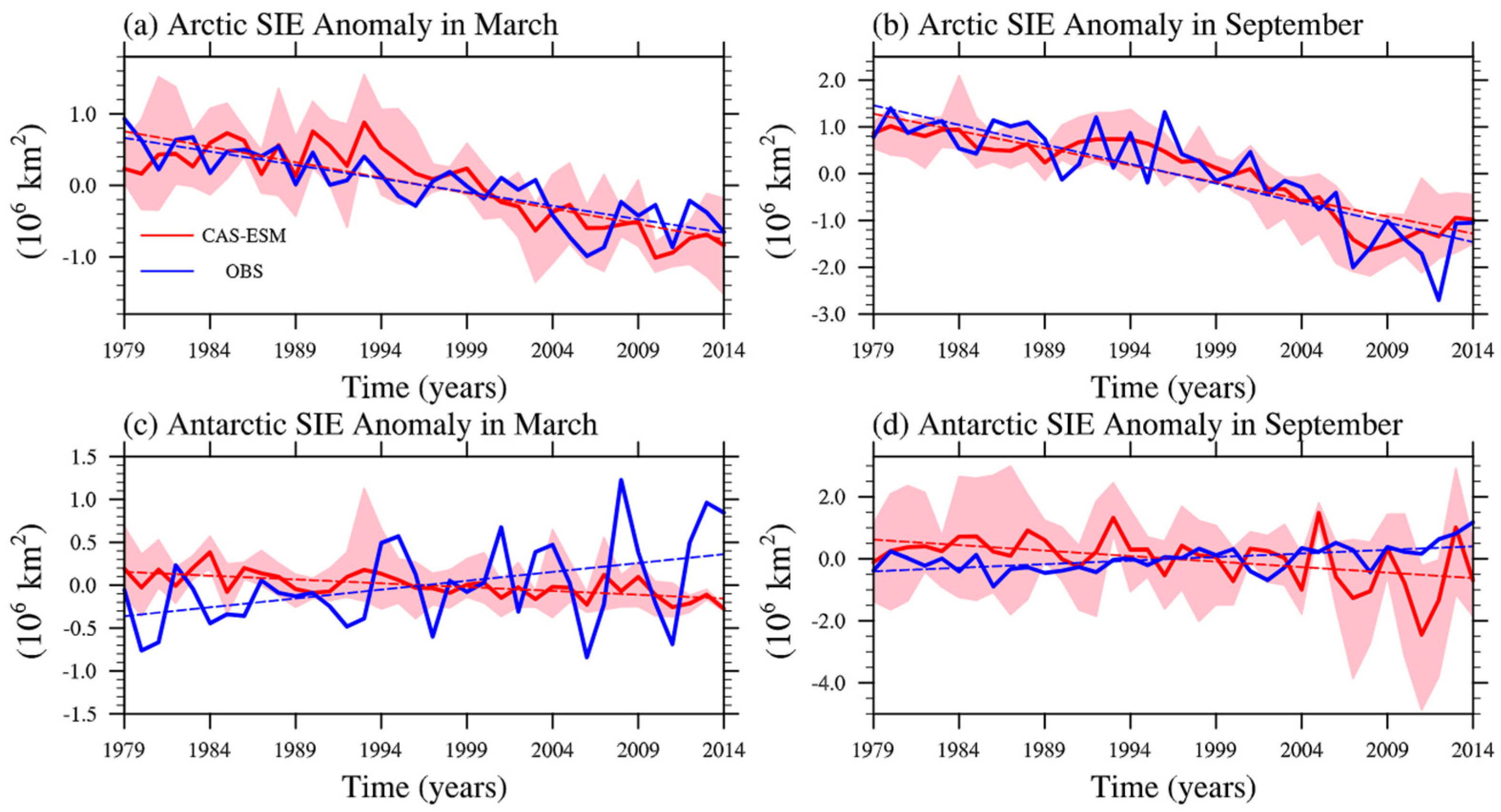
3.1. Sea Ice Extent (SIE)

Figure 1 shows the temporal evolution of March and September sea ice extent (SIE) anomalies in the Arctic and Antarctic in the historical simulation. For the Arctic SIE, the observed and modelled linear trends of March and September are very similar (Figure 1). The March and September Arctic SIE trends from CAS-ESM 2.0 for 1979 to 2014 are −0.42 million and −0.73 million km2 per decade, respectively. The corresponding observed values are −0.73 million and −0.83 million km2 per decade, respectively. The Arctic trends for March and September in 1979–2014 are very close to the median values of −0.45 million and −0.70 million km2 per decade in CMIP6 historical simulations [29]. It should be noted that the declining trend of Arctic SIE in September simulated for 2000 to 2014 is smaller than the observed value, which is a common phenomenon in CMIP6 simulations [29]. For 2000 to 2014, the September Arctic SIE trends from National Snow and Ice Data Center (NSIDC) and CAS-ESM 2.0 are −1.39 million and −0.95 million km2 per decade, respectively.
For the Antarctic, CAS-ESM 2.0 exhibited a slightly negative trend for March and September, whereas the observation was a weak but significant positive trend, which is a persistent problem in CMIP5 and CMIP6 models [29,30,31]; this may be because the models fail to represent sea ice physics [31]. The observed Antarctic SIE trends during March and September in 1979–2014 are 0.21 million and 0.23 million km2 per decade, respectively, whereas CAS-ESM 2.0 shows negative trends, with values of −0.09 million and −0.35 million km2 per decade, respectively. The modelled Antarctic trend for September in 1979–2014 is very close to the median value of −0.43 million km2 per decade in CMIP6 historical simulations [29].
The annual mean seasonal cycle of Arctic and Antarctic SIE from CAS-ESM 2.0 during 1979 to 2014 is shown in Figure 2, with the observed climatology of those years for comparison. It indicates that CAS-ESM 2.0 can adequately reproduce the observed SIE seasonal cycle in the Arctic and Antarctic, reaching the maximum in March in the Arctic and September in the Antarctic and the minimum in September and February in both hemispheres. For both hemispheres, the amplitude of the seasonal cycle is larger in terms of winter–summer SIE difference relative to observations: the SIE in summer is underestimated (June–August in Arctic, December–February in Antarctic), while the SIE in winter is overestimated (June–August in Antarctic, December–February in Arctic), which is consistent with the CAS-ESM 2.0 simulation of coupled ocean and sea ice components [19]. As Figure 2 shows, the model’s large underestimation for the Arctic occurs in August and September and overestimation occurs between January and May. For the Antarctic, the underestimation occurs between January and June and the overestimation between August and October. March SIE values from observations and CAS-ESM 2.0 for the Arctic and Antarctic are 15.26, 16.92, 4.02, and 0.53 million km2, respectively, and the corresponding values of multi-model mean in CMIP6 are 17.08 and 2.79 million km2 [29]. September SIE values from observations and CAS-ESM 2.0 for the Arctic and Antarctic are 5.99, 3.50, 18.53, and 23.15 million km2, respectively, and the corresponding values of the multi-model mean in CMIP6 are 7.18 and 17.47 million km2 [29]. The results indicate higher seasonal variation in the model for both hemispheres relative to observations, which is a common phenomenon in many contemporary coupled models [29]. We will discuss the reason in the following sections, which will provide insights for improving the sea ice simulation performance of other coupled models. The SIE biases of CAS-ESM 2.0 for the Arctic and Antarctic are different, with relatively larger bias in summer than winter in the Arctic and smaller bias in summer than winter in the Antarctic. SIE biases for the Arctic and Antarctic in March are 1.66 and −3.49 million km2, respectively, and the corresponding values in September are −2.49 and 4.62 million km2. The comparison shows that the Antarctic has larger biases than the Arctic. The root mean square (RMS) difference between CAS-ESM 2.0 and observed monthly seasonal cycles of Arctic and Antarctic SIE climatology are 1.46 × 10⁶ km2 and 3.09 × 10⁶ km2, respectively. These values are very close to the median RMS error of 1.45 × 10⁶ km2 and 3.42 × 10⁶ km2 of CMIP5 historical simulations of sea ice [30].

3.2. Sea Ice Concentration

The simulated spatial distributions of sea ice concentration in March and September based on the 1979–2014 average for both hemispheres are shown in Figure 3 and Figure 4, along with Special Sensor Microwave Imager (SSMI) observations based on the 1980–2014 average for comparison [33]. CAS-ESM 2.0 can reasonably reproduce the spatial distribution of March sea ice concentration in the Arctic region (Figure 3b). Compared with the observations, the large biases are mainly distributed in the margin of sea ice cover. There is an overestimation of sea ice concentration over the Bering Sea, Okhotsk Sea, Barents Sea, and Greenland–Iceland–Norway region and an underestimation over the Labrador Sea, especially for the coastline. On the contrary, in March, the CAS-ESM 2.0 simulation shows less sea ice in the whole Southern Ocean compared to the observations, and the sea ice almost completely disappeared, which is in strong contrast to the observations. For September, CAS-ESM 2.0 reproduces a lower concentration in most regions compared with the observations, especially in the Beaufort Sea, Canada Basin, and central Arctic Ocean, while the simulated sea ice concentration is slightly larger in the Greenland Sea and Barents Sea. For the Southern Ocean in September, the CAS-ESM 2.0 simulation generally resembles the observed sea ice concentration pattern, except for expanding northward ice over the Weddell Sea and Ross Sea and shrinking southward ice over the southeast Indian Ocean and southern Pacific Ocean.

3.3. Atmospheric and Oceanic Forcings Related to Sea Ice

Previous studies have shown that the SAT and SST involved in the thermodynamic processes of sea ice have dominant influence on sea ice evolution [33,34]. Figure 5 and Figure 6 show the annual mean seasonal SAT and SST cycles in the Arctic and Antarctic from 1979 to 2014 in CAS-ESM 2.0. The summer (winter) SAT and SST in both hemispheres are warmer (colder) than the observations. The corresponding SAT and SST biases in northern hemisphere are 1.38 °C (−4.03 °C) and 1.36 °C (−0.19 °C), respectively, and the corresponding values in the southern hemisphere are 3.49 °C (−1.17 °C) and 2.21 °C (−0.14 °C), respectively. This would result in an underestimation of SIE in summer and an overestimation of SIE in winter in both hemispheres (Figure 2). In order to further explore the effects of ocean and atmosphere forcing on sea ice, Figure 7 and Figure 8 present the spatial patterns of SAT and SST in March and September. In the Arctic in March, the colder biases of SAT and SST in CAS-ESM 2.0 relative to the observations are mainly located in the Okhotsk Sea and Barents Sea, along with too large sea ice in these regions (Figure 3), while the warmer biases are along the Labrador Sea coast, with underestimated sea ice concentration (Figure 3). The simulated SAT and SST in CAS-ESM 2.0 show warmer biases in the whole Southern Ocean relative to the observations, which is consistent with the underestimated sea ice (Figure 3). In September, the CAS-ESM 2.0 simulation shows warmer SAT and SST biases in the Beaufort Sea, Canada Basin, and southern Indian Ocean, accompanied by a sea ice concentration that is too low (Figure 4). The colder biases of SAT and SST in CAS-ESM 2.0 mainly appeared in the Greenland Sea, Barents Sea, Weddell Sea, and Ross Sea, which is consistent with the sea ice concentration biases in these regions. This indicates that SST and SAT play important roles in sea ice evolution, which is consistent with previous studies [33,34].

3.4. Sea Ice Thickness and Motion

In contrast with the relatively long-term observations of sea ice concentration, observations of sea ice thickness are of insufficient duration and have large uncertainty. A newly merged sea ice thickness product from the CryoSat-2 and SMOS satellites (CS2SMOS), which covers both thin and thick ice in the Arctic by using an optimal interpolation scheme based on the uncertainties of the individual products and modelled spatial error covariance [37], is used here to compare simulations of ice thickness. Data of Arctic sea ice thickness in the freezing season (October–April) are available from November 2010, and the average of 2010–2019 served as the climatological observation, although sea ice has been thinning since 1979 [38]. As shown in Figure 9, CAS-ESM 2.0 well simulates the reduced ice thickness gradient from the central Arctic to the Siberian Sea, but fails to present thicker ice north of Greenland and the Canadian Archipelago, where multi-year ice is located. Most likely, the Arctic pole in the grid distribution becomes a barrier that prevents ice from flowing into the “thick ice” area. The annual mean ice volume for the whole Arctic reaches a maximum of 25.25 × 10³ km3 in April and a minimum of 5.15 × 10³ km3 in September. Compared with the Arctic monthly ice volume data from the Pan-Arctic Ice Ocean Modeling and Assimilation system (PIOMAS) [39], the simulation of averaged ice volume in CAS-ESM2.0 is smaller overall.
Despite the grid issues, CAS-ESM 2.0 successfully captures the two primary components of Arctic sea ice motion, the Beaufort Gyre by an anticyclonic regime and the polar transport stream by ice moving from the Siberian coast of Russia across the Arctic basin into the Greenland Sea (Figure 10a,b). The large-scale clockwise circulation of ice around Antarctica is also presented in the simulations, with northward movement on average and gyres in the Ross Sea and small rotation in the Weddell Sea (Figure 10c,d).

3.5. Sea Ice Mass Budget

To further understand the main physical drivers that govern the evolution of sea ice, the sea ice mass budget in both hemispheres was evaluated [41]. Figure 11 shows the average seasonal and annual mean sea ice mass budget over the sea ice-covered Arctic and Antarctic regions, including ice growth or loss due to basal growth, frazil ice formation, top ice melt, basal ice melt, lateral ice melt, snow-to-ice conversion, dynamics, and the total of these processes. In general, the Arctic (Antarctic) sea ice mass shows a balance of net gain from September to April (March to September) and a net loss from May to September (October to February).
The Arctic ice mass increase is mainly due to basal growth, which accounts for 85.3% of total annual growth. Frazil ice formation is a secondary contributor (13.4%) to ice growth, and the small remainder is snow–ice formation. This is very similar to the Arctic ice growth contributions reported in Keen et al. [42]. The maximum ice melt occurs in June, with top melt peaking at this time, one month earlier than the simulations of 14 models in CMIP6 [42], and dramatic ice loss is ongoing in June, with basal melt peaking at this time. Additionally, heat from the ocean continuously melts ice, especially in May to September. This indicates that too large sea ice in the Arctic winter mainly results from the ocean effect, and too low sea ice in the Arctic summer can be attributed to the combined effects of atmosphere–ice and ocean–ice interactions. For the annual mean ice loss, ice melt at the base and top surface accounts for a considerable amount (basal melt, 51.5%; top melt, 43.6%), with a small contribution from lateral melt (4.4%).
The Antarctic ice growth is also mainly attributed to basal growth, which reaches the maximum in July–August, representing 73.7% of the total annual ice mass increase. The processes of frazil ice formation in open water and snow–ice formation contribute 15.3 and 11.0%, respectively, to ice mass growth. The Antarctic ice mass loss reaches the maximum in December, with basal and top melt peaking this time, and heat from ocean melts accounts for 82.1% of the total annual ice melt, along with 14.7% from top melt and 3.1% from lateral melt. This suggests that the ocean–ice interaction effect plays a dominant role in the bias of sea ice in winter and summer in the Antarctic.

4. Conclusions and Discussion

By comparing observed data with historical simulation, we show that in the Arctic and Antarctic CAS-ESM 2.0 is able to simulate the annual variability of SIE in March and September well. CAS-ESM 2.0 reproduces reasonable seasonal cycle features and the climatological spatial distribution of Arctic and Antarctic sea ice, including SIE, sea ice concentration, sea ice thickness, and motion. However, SIE in CAS-ESM 2.0 is too large in winter and too low in summer in both hemispheres, indicating higher seasonal variation in the model relative to observations, which is consistent with the simulation of coupled ocean and sea ice components of CAS-ESM 2.0.
The overestimated winter sea ice concentration in the Arctic is mainly located in Bering Sea, Okhotsk Sea, Barents Sea, and Greenland–Iceland–Norway region, and the negative sea ice concentration bias is in the Labrador Sea, especially the coastline. Surrounding the Antarctic, the summer sea ice concentration is underestimated in the whole Southern Ocean, and the overestimation of winter sea ice concentration occurs in regions of the Southern Ocean that are connected with the Atlantic Ocean. The sea ice biases are mainly consistent with the corresponding SAT and SST biases. The Arctic sea ice thickness simulated by CAS-ESM 2.0 is lower overall compared to the observations. The primary characterizations of ice motion in the Arctic by the Beaufort Gyre and polar transport stream and in the Antarctic by the circumpolar current are successfully reproduced in CAS-ESM2.0.
As for the sea ice mass budget, in both hemispheres over the whole year, basal growth contributes the most to ice increase in the cold season, followed by frazil ice formation. Snow-to-ice formation contributes only a small amount in the Arctic but a comparable amount to frazil ice formation in the Antarctic. Thus, the ocean–ice interaction (colder SST bias relative to observations) is most likely an important factor for too large SIE in winter in both hemispheres. Basal melt and top melt make comparable contributions to Arctic ice loss, followed by lateral melt, while most Antarctic ice loss is due to heat from the ocean, followed by top melt and lateral melt, which indicates the importance of ocean–ice and air–ice interactions (warmer SST and SAT biases relative to observations) in the underestimation of sea ice in the Arctic summer and the dominance of ocean–ice interactions in too large sea ice in the Antarctic winter. Therefore, inaccuracies in atmosphere and ocean components, especially ocean components, may present limitations in terms of the ability of CAS-ESM 2.0 to simulate sea ice. Improving the atmosphere and ocean models in terms of both horizontal resolution and physical parameterization is the next step in model development for CAS-ESM 2.0. Moreover, waves have a significant impact on simulations of Arctic and Antarctic ice through wave stresses and wave motions, and on improving SST simulation [43,44,45,46], while the wave–ice interaction is absent in CAS-ESM 2.0, thus incorporating a wave model in CAS-ESM 2.0 is also part of our further work.

Author Contributions

Conceptualization, X.G.; methodology, P.F., J.J. and J.H.; writing—original draft preparation, X.G. and M.S.; writing—review and editing, P.F., M.S. and J.J.; visualization, P.F. and M.S.; supervision, J.J., H.Z. and K.F.; project administration, M.Z. and Q.Z.; funding acquisition, J.J. and M.Z. All authors have read and agreed to the published version of the manuscript.

Funding

This research was supported by the National Key R&D Program of China (2018YFA0605901), the National Natural Science Foundation of China (Grant Nos. 42005123 and 41941009), the Youth Innovation Promotion Association of CAS (2022074), and the National Key Scientific and Technological Infrastructure project “Earth System Science Numerical Simulator Facility” (EarthLab). Simulations were performed on supercomputers provided by the Big Earth Data Science Platform.

Institutional Review Board Statement

Not applicable.

Informed Consent Statement

Not applicable.

Data Availability Statement

Not applicable.

Acknowledgments

We thank the three anonymous reviewers for their constructive comments and suggestions which helped to improve the quality of this manuscript. This work is jointly supported by the National Key R&D Program of China (2018YFA0605901), the Youth Innovation Promotion Association of CAS (2022074), the National Natural Science Foundation of China (Grant Nos. 42005123 and 41941009), and the National Key Scientific and Technological Infrastructure project “Earth System Science Numerical Simulator Facility” (EarthLab).

Conflicts of Interest

The authors declare no conflict of interest.

References

  1. IPCC. Summary for Policymakers. In IPCC Special Report on the Ocean and Cryosphere in a Changing Climate; Pörtner, H.-O., Roberts, D.C., Masson-Delmotte, V., Zhai, P., Tignor, M., Poloczanska, E., Mintenbeck, K., Alegría, A., Nicolai, M., Okem, A., et al., Eds.; IPCC: Geneva, Switzerland, 2019. [Google Scholar]
  2. Stroeve, J.; Holland, M.M.; Meier, W.; Scambos, T.; Serreze, M. Arctic sea ice decline: Faster than forecast. Geophys. Res. Lett. 2007, 34, L09501. [Google Scholar] [CrossRef]
  3. Liu, J.; Song, M.; Horton, R.M.; Hu, Y. Reducing spread in climate model projections of a September ice-free Arctic. Proc. Natl. Acad. Sci. USA 2013, 110, 12571–12576. [Google Scholar] [CrossRef] [PubMed] [Green Version]
  4. Turner, J.; Comiso, J. Solve Antarctica’s sea-ice puzzle. Nature 2017, 547, 275–277. [Google Scholar] [CrossRef] [PubMed]
  5. Durner, G.M.; Douglas, D.C.; Nielson, R.M.; Amstrup, S.C.; McDonald, T.L.; Stirling, I.; Mauritzen, M.; Born, E.W.; Wiig, Ø.; DeWeaver, E.; et al. Predicting 21stcentury polar bear habitat distribution from 647 global climate models. Ecol. Monogr. 2009, 79, 25–58. [Google Scholar] [CrossRef]
  6. Zhang, X.; Zeng, Q. A computational design of numerical world general circulation model. Chinese J. Atmos. Sci. 1988, 12, 149–165. (In Chinese) [Google Scholar]
  7. Zeng, Q.; Zhang, X.; Liang, X.; Yuan, C.; Chen, S. Documentation of IAP Two-Level Atmospheric General Circulation Model; 1989. [Google Scholar]
  8. Dai, Y.; Zeng, Q. A land surface model (IAP94) for climate studies part i: Formulation and validation in off-line experiments. Adv. Atmos. Sci. 1997, 14, 433–460. [Google Scholar]
  9. Zhou, G.; Zhang, Y.; Jiang, J.; Zhang, H.; Wu, B.; Cao, H.; Wang, T.; Hao, H.; Zhu, J.; Yuan, L.; et al. Earth System Model: CAS-ESM. Front. Data Comput. 2020, 2, 38–54. (In Chinese) [Google Scholar]
  10. Zhang, H.; Zhang, M.; Jin, J.; Fei, K.; Ji, D.; Wu, C.; Zhu, J.; He, J.; Chai, Z.; Xie, J.; et al. Description and Climate Simulation Performance of CAS-ESM Version 2. J. Adv. Model. Earth Syst. 2020, 12, e2020MS002210. [Google Scholar] [CrossRef]
  11. Liu, H.; Lin, P.; Yu, Y.; Zhang, X. The baseline evaluation of LASG/IAP climate system ocean model (LICOM) version 2.0. Acta Meteorol. Sin. 2012, 26, 318–329. [Google Scholar] [CrossRef]
  12. Dai, Y.; Zeng, X.; Dickinson, R.E.; Baker, I.; Bonan, G.B.; Bosilovich, M.G.; Denning, S.; Dirmeyer, P.; Houser, P.R.; Niu, G. The Common Land Model (CLM). B. Am. Meteorol. Soc. 2003, 84, 1013–1023. [Google Scholar] [CrossRef] [Green Version]
  13. Hunke, E.C.; Lipscomb, W.H. CICE: The Los Alamos Sea Ice Model User’s Manual, Version 4; LA-CC-06-012; Los Alamos National Laboratory Tech. Rep.: Los Alamos, NM, USA, 2008. [Google Scholar]
  14. He, J.; Zhang, M.; Lin, W.; Colle, B.; Vogelmann, A.M. Simulations of a mid-latitude cyclone over the southern Great Plains usingthe WRF nested within the CESM. J. Adv. Model. Earth Syst. 2013, 5, 611–622. [Google Scholar] [CrossRef]
  15. Zhu, J.; Zeng, X.; Zhang, M.; Dai, Y.; Ji, D.; Li, F.; Zhang, Q.; Zhang, H.; Song, X. Evaluation of the new dynamic global vegetation model in CAS-ESM. Adv. Atmos. Sci. 2018, 35, 659–670. [Google Scholar] [CrossRef]
  16. Li, F.; Zeng, X.; Levis, S. A process-based fire parameterization of intermediate complexity in a Dynamic Global Vegetation Model. Biogeosciences 2012, 9, 2761–2780. [Google Scholar] [CrossRef] [Green Version]
  17. Chen, H.; Wang, Z.; Li, J.; Tang, X.; Ge, B.; Wu, X.; Wild, O.; Carmichael, G.R. GNAQPMS-Hg v1.0, a global nested atmospheric mercury transport model: Model description, evaluation and application to trans-boundary transport of Chinese anthropogenic emissions. Geocsic. Model. Dev. 2015, 8, 2857–2876. [Google Scholar] [CrossRef] [Green Version]
  18. Dong, X.; Jin, J.; Liu, H.; Zhang, H.; Zhang, M.; Lin, P.; Zeng, Q.; Zhou, G.; Yu, Y.; Song, M.; et al. CAS-ESM2.0 Model Datasets for CMIP6 Ocean Model Intercomparison Project Phase 1 (OMIP1). Adv. Atmos. Sci. 2021, 38, 307–316. [Google Scholar] [CrossRef]
  19. Jin, J.; Zeng, Q.; Wu, L.; Liu, H.; Zhang, M. Formulation of a new ocean salinity boundary condition and impact on the simulated climate of an oceanic general circulation model. Sci. China Earth Sci. 2017, 60, 491–500. [Google Scholar] [CrossRef]
  20. Fairall, C.W.; Bradley, E.F.; Hare, J.E.; Grachev, A.A.; Edson, J.B. Bulk parameterization of air–sea fluxes: Updates and verification for the COARE algorithm. J. Clim. 2003, 16, 571–591. [Google Scholar] [CrossRef]
  21. Hunke, E.C.; Dukowicz, J.K. An elasticviscous-plastic model for sea ice dynamics. J. Phys. Oceanogr. 1997, 27, 1849–1867. [Google Scholar] [CrossRef] [Green Version]
  22. Lipscomb, W.H.; Hunke, E.C.; Maslowski, W.; Jakacki, J. Ridging, strength, and stability in high-resolution sea ice models. J. Geophys. Res. 2007, 112, C03S91. [Google Scholar] [CrossRef]
  23. Lipscomb, W.H.; Hunke, E.C. Modeling sea ice transport using incremental remapping. Mon. Weather Rev. 2004, 132, 1341–1354. [Google Scholar] [CrossRef]
  24. Collins, W.D.; Bitz, C.M.; Blackmon, M.L.; Bonan, G.B.; Bretherton, C.S.; Carton, J.A.; Chang, P.; Doney, S.C.; Hack, J.J.; Henderson, T.B.; et al. The community climate system model version 3 (CCSM3). J. Clim. 2006, 19, 2122–2143. [Google Scholar] [CrossRef]
  25. Ji, D.; Wang, L.; Feng, J.; Wu, Q.; Cheng, H.; Zhang, Q.; Yang, J.; Dong, W.; Dai, Y.; Gong, D.; et al. Description and basic evaluation of Beijing Normal University Earth System Model (BNU-ESM) version 1. Geosci. Model. Dev. 2014, 7, 2039–2064. [Google Scholar] [CrossRef] [Green Version]
  26. Dai, Y.; Dickinson, R.E.; Wang, Y. A Two-Big-Leaf model for canopy temperature, Photosynthesis, and Stomatal conductance. J. Clim. 2004, 17, 2281–2299. [Google Scholar] [CrossRef]
  27. Zeng, X.; Li, F.; Song, X. Development of the IAP dynamic global vegetation model. Adv. Atmos. Sci. 2014, 31, 505–514. [Google Scholar] [CrossRef]
  28. Eyring, V.; Bony, S.; Meehl, G.A.; Senior, C.A.; Stevens, B.; Stouffer, R.J.; Taylor, K.E. Overview of the Coupled Model Intercomparison Project Phase 6 (CMIP6) experimental design and organization. Geosci. Model. Dev. 2016, 9, 1937–1958. [Google Scholar] [CrossRef] [Green Version]
  29. Shu, Q.; Wang, Q.; Song, Z.; Qiao, F.; Zhao, J.; Chu, M.; Li, X. Assessment of Sea Ice Extent in CMIP6 with Comparison to Observations and CMIP5. Geophys. Res. Lett. 2020, 47, e2020GL087965. [Google Scholar] [CrossRef]
  30. Shu, Q.; Song, Z.; Qiao, F. Assessment of sea ice simulations in the CMIP5 models. Cryosphere 2015, 9, 399–409. [Google Scholar] [CrossRef] [Green Version]
  31. Turner, J.; Bracegirdle, T.J.; Phillips, T.; Marshall, G.J.; Hosking, J.S. An initial assessment of Antarctic sea ice extent in the CMIP5 models. J. Clim. 2013, 26, 1473–1484. [Google Scholar] [CrossRef]
  32. Cavalieri, D.J.; Parkinson, C.L.; Gloersen, P.; Zwally, H.J. Sea ice concentrations from Nimbus-7 SMMR and DMSP SSM/I-SSMIS Passive Microwave Data, Version 1; NASA DAAC at the National Snow and Ice Data Center: Boulder, CO, USA, 1996. [Google Scholar] [CrossRef]
  33. Comiso, J.C. Bootstrap Sea Ice Concentrations from Nimbus-7 SMMR and DMSP SSM/I-SSMIS, Version 3; NASA National Snow and Ice Data Center Distributed Active Archive Center: Boulder, CO, USA, 2017. [Google Scholar]
  34. Zhang, J.; Woodgate, R.; Moritz, R. Sea ice response to atmospheric and oceanic forcing in the Bering Sea. J. Phys. Oceanogr. 2010, 40, 1729–1747. [Google Scholar] [CrossRef]
  35. Compo, G.P.; Whitaker, J.S.; Sardeshmukh, P.D.; Matsui, N.; Allan, R.J.; Yin, X.; Gleason, B.E.; Vose, R.S.; Rutledge, G.; Bessemoulin, P.; et al. The Twentieth Century Reanalysis Project. Q. J. Roy. Meteor. Soc. 2011, 137, 1–28. [Google Scholar] [CrossRef]
  36. Mishonov, A. World Ocean Atlas 2013 Product Documentation; Boyer, T., Ed.; NOAA: Washington, DC, USA, 2013. [Google Scholar]
  37. Ricker, R.; Hendricks, S.; Kaleschke, L.; Tian-Kunze, X.; King, J.; Haas, C. A weekly Arctic sea-ice thickness data record from merged CryoSat-2 and SMOS satellite data. Cryosphere 2017, 11, 1607–1623. [Google Scholar] [CrossRef] [Green Version]
  38. Kwok, R. Arctic sea ice thickness, volume, and multiyear ice coverage: Losses and coupled variability (1958–2018). Environ. Res. Lett. 2018, 13, 105005. [Google Scholar] [CrossRef]
  39. Zhang, J.; Rothrock, D.A. Modeling global sea ice with a thickness and enthalpy distribution model in generalized curvilinear coordinates. Mon. Wea. Rev. 2003, 131, 845–861. [Google Scholar] [CrossRef] [Green Version]
  40. Tschudi, M.A.; Meier, W.N.; Stewart, J.S. An enhancement to sea ice motion and age products at the National Snow and Ice Data Center (NSIDC). Cryosphere 2020, 14, 1519–1536. [Google Scholar] [CrossRef]
  41. Notz, D.; Jahn, A.; Holland, M.; Hunke, E.; Massonnet, F.; Stroeve, J. The CMIP6 Sea-Ice Model Intercomparison Project (SIMIP): Understanding sea ice through climate-model simulations. Geosci. Model. Dev. 2016, 9, 3427–3446. [Google Scholar] [CrossRef] [Green Version]
  42. Keen, A.; Blockley, E.; Bailey, D.A.; Debernard, J.B.; Bushuk, M.; Delhaye, S.; Docquier, D.; Feltham, D.; Massonnet, F.; O’Farrell, S.; et al. An inter-comparison of the mass budget of the Arctic sea ice in CMIP6 models. Cryosphere 2021, 15, 951–982. [Google Scholar] [CrossRef]
  43. Song, Z.; Qiao, F.; Song, Y. Response of the equatorial basin-wide SST to non-breaking surface wave-induced mixing in a climate model: An amendment to tropical bias. J. Geophys. Res. 2012, 7, C00J26. [Google Scholar] [CrossRef]
  44. Stopa, J.E.; Sutherland, P.; Ardhuin, F. Strong and highly variable push of ocean waves on Southern Ocean sea ice. Proc. Natl. Acad. Sci. USA 2018, 115, 5861–5865. [Google Scholar] [CrossRef] [Green Version]
  45. Holland, P.R. The seasonality of Antarctic sea ice trends. Geophys. Res. Lett. 2014, 41, 4230–4237. [Google Scholar] [CrossRef] [Green Version]
  46. Bruno, M.S.; Madsen, O.S. Coupled circulation and ice floe movement model for partially ice-covered continental shelves. J. Geophys. Res. 1989, 94, 2065–2077. [Google Scholar] [CrossRef]
Figure 1. Time evolution of ensemble mean SIE anomalies in Arctic and Antarctic in historical simulation. The figures (a,b) show the anomaly in Arctic SIE in March and September respectively, and the figures (c,d) show the corresponding Antarctic. Red and blue lines indicate CAS-ESM 2.0 and observations, respectively. Anomalies were calculated from 1979–2014 average. Pink areas represent simulated anomaly ranges of four simulations. Dashed lines represent linear trend of CAS-ESM 2.0 and observations. SIE is areal sum of all grid points whose sea ice concentration exceeds 15%.
Atmosphere 13 01056 g001
Figure 2. Seasonal cycles of (a) Arctic and (b) Antarctic SIE climatology (106 km2) computed from simulated ensemble mean for 1979–2014 in historical simulation (red), satellite observations (black), and their biases (blue). The red and black curves correspond to the left axis, and the blue curve refers to the right axis. Observed data are from NSIDC [32]. SIE is areal sum of all grid points whose sea ice concentration exceeds 15%.
Atmosphere 13 01056 g002
Figure 3. Spatial patterns of (a,c) SSMI observations from March 1980–2014 and (b,d) CAS-ESM 2.0 ensemble mean sea ice concentrations for March 1979–2014 in historical simulation, in Northern Hemisphere (upper panel) and Southern Hemisphere (lower panel).
Atmosphere 13 01056 g003
Figure 4. Spatial patterns of (a,c) SSMI observations from September 1980–2014 and (b,d) CAS-ESM 2.0 ensemble mean sea ice concentrations for September 1979–2014 in historical simulation, in Northern Hemisphere (upper panel) and Southern Hemisphere (lower panel).
Atmosphere 13 01056 g004
Figure 5. Comparison between CAS-ESM 2.0 and NCEP [35] observations for seasonal SAT cycle in 1979–2014 in (a) Northern Hemisphere (north of 45° N) and (b) Southern Hemisphere (south of 45° S).
Atmosphere 13 01056 g005
Figure 6. Comparison between CAS-ESM 2.0 and WOA 13 [36] observations for seasonal SST cycle in 1979–2014 in (a) Northern Hemisphere and (b) Southern Hemisphere.
Atmosphere 13 01056 g006
Figure 7. Spatial patterns of SAT bias relative to NCEP data [35] in (a,c) March and (b,d) September in the Arctic (upper panel) and Antarctic (lower panel).
Atmosphere 13 01056 g007
Figure 8. Spatial patterns of simulated ensemble mean in 1979–2014: (a,b) in the Arctic in March and September, and (c,d) in the Antarctic in March and September, with SST bias relative to WOA 13 [36].
Atmosphere 13 01056 g008
Figure 9. Average ice thickness during freezing season from (a) CS2SMOS observations during 2010–2019 and (b) CAS-ESM 2.0 for ensemble mean of 1979–2014 historical simulation in the Northern Hemisphere, and (c) simulated average ice volume in the Arctic during 1979–2014.
Atmosphere 13 01056 g009
Figure 10. Annual mean ice motion direction (vector) and speed (shading) based on NASA NSIDC observations [40] for (a,c) 1979–2014 climatology and (b,d) CAS-ESM 2.0 historical simulations for ensemble mean of 1979–2014 in Northern Hemisphere (upper panel) and Southern Hemisphere (lower panel).
Atmosphere 13 01056 g010
Figure 11. (a,c) Seasonal cycle of monthly mean value and (b,d) annual mean value of sea ice mass budget for Arctic (a,b) and Antarctic (c,d) regions for ensemble mean of 1979–2014.
Atmosphere 13 01056 g011
Publisher’s Note: MDPI stays neutral with regard to jurisdictional claims in published maps and institutional affiliations.

