Abstract
This paper presents a passive bistatic radar (PBR) configuration using a global navigation satellite system as an illuminator of opportunity for the rotor blade feature extraction of a helicopter. Aiming at the strong fixed clutter in the surveillance channel of the PBR, a novel iteration clutter elimination method-based singular-value decomposition approach is proposed. Instead of the range elimination method used in the classic extended cancellation algorithm, the proposed clutter elimination method distinguishes the clutter using the largest singular value and by remove this value. At the same time, the fuselage echo of the hovering helicopter can also be suppressed along with the ground clutter, then the rotor echo of this can be obtained. In the micro-motion feature extraction, the mathematic principle of the flash generation process in the time–frequency distribution (TFD) is derived first. Next, the phase compensation method is applied to achieve the time–frequency flash shift in the TFD. After this, the center frequencies of the standard flashes in the TFD are compared with the standard frequency dictionary. The mean l1 norm is utilized to estimate the feature parameters of the helicopter rotor. In the experiments, the scattering point model and the physical optics facet model demonstrate that the proposed method can obtain more accurate parameter estimation results than some classic algorithms.
1. Introduction
Based on their illuminators, radar systems can be categorized as active or passive. Active radar systems utilize transmitters with known locations, while passive systems exploit illuminators of opportunity (IO) with limited knowledge [1,2]. In comparison to the active radar systems, the passive systems are low in cost, size, weight, and power; they exhibit lower manufacturing and operational costs due to the lack of emitting elements [3,4]. Furthermore, depending on the relative location between the transmitter and receiver, the radar systems can also be categorized as monostatic or bistatic [5]. The employed location of the IO is always known, but the receiver is always employed on the basis of the functional requirements, meaning a passive radar is always a passive bistatic radar (PBR). In recent years, the interest in exploiting global navigation satellite systems (GNSSs) for remote sensing has been growing on account of the advantages of its high coverage of the entire Earth [6]. For hovering targets, such as helicopters and drones at low altitude, it is difficult for ground radar systems to detect these targets, and airborne-based radars may act as a supplement for the blind areas to ground-based radars [7,8,9]. The exploitation of the GNSS for target recognition and imaging has been reported in [10]; however, the main limitation is the weak target echo in the surveillance channel.
Coherent integration (CI) is always implemented to enhance the target echo energy to achieve target detection, which means that the PBR contains two receiving channels: the reference channel and surveillance channel. The former is applied to receive the direct-path signal, and the latter us used for the target echo, which of course is mixed with noise and clutter. Additionally, the target echo energy is far lower than the direct-path signal and multipath clutter [11,12,13]. Hence, clutter cancellation is an essential step for target detection or recognition in PBR. The existing clutter cancellation methods for PBR mainly address clutter from the time domain or frequency domain. The extended cancellation algorithm (ECA) proposed by Colone in the literature [14] uses the reference antenna to receive the direct-path signal, and then the clutter subspace is constructed. Taking advantage of the orthogonal relationship between the target echo and ground clutter, the surveillance signal is projected in the orthocomplement of the clutter subspace to achieve clutter suppression. The ECA can remove the clutter from the surveillance signal to a certain degree. However, the method needs to calculate the matrix inversion that leads to heavy computational burden, which cannot satisfy the requirements for real-time target detection. Otherwise, Bi et al. employed singular-value decomposition (SVD) to select appropriate singular values and characteristic components corresponding to the effective signals for signal reconstruction [15]. An SVD method based on the Hankel matrix in the local frequency domain was proposed to suppress the random noise. Besides the direct signal and ground clutter, in rotor feature extraction, the fuselage echo of a helicopter also needs to be suppressed. When the helicopter is hovering in the air, the fuselage also has no motion and the echo can be suppressed as ground clutter as well. Then, the remaining rotor echo in the surveillance channel can be utilized to extract the micro-motion features of the helicopter.
Target micro-motions such as rotating rotors of helicopters introduce micro-Doppler (mD) frequencies in the received signal, and the mD component is close related to the target features [16,17,18]. When a helicopter is hovering, the traditional target detection methods based on CI become invalid [19]. At this time, the mD features of the helicopter rotor can provide much more information for target detection and recognition [20,21,22,23,24]. As a result, the mD analysis algorithm in GNSS-based PBR can play an important role in helicopter detection, classification, and recognition.
Various methods have been presented for mD feature extraction by utilizing a signal model or time-frequency (TF) transform. Deng et al. in [25] proposed a parameter estimation method based on the generalized likelihood ratio test (GLRT), while the parameter estimation accuracy heavily depends on the orthogonality of the signal space with different parameters. Oh et al. introduced empirical mode decomposition (EMD) to extract the features for automatic multicategory mini-unmanned aerial vehicle (UAV) classification [26]. However, this method is restricted by the end effect and model mixing. Another study [27] reported a technique for the imaging of fast-rotating blades based on the orthogonal matching pursuit (OMP) method. Another paper [28] presented the relationships between the carrier frequency and the mD effect, whereby the wavelength can affect the maximum mD frequency remarkably. The Hough–Radon transform (HRT) is applied to extract the target features parameters. However, this method ignores the flashes that can deteriorate the estimation effectiveness in the time–frequency distribution (TFD). The mD of a helicopter with different blade tip shapes is analyzed in [29], which can provide supplementary information for helicopter identification. The independent component algorithm (ICA) was introduced in [30] to separate each blade to extract the rotor features. Of all these methods, the TF analysis is the most commonly used approach and provides the time-varying Doppler frequency characteristics of signals.
Hence, in this paper, the feature extraction of a helicopter based on the TFD is considered after fixed clutter suppression. Firstly, aiming at the strong clutter in a PBR, the iteration elimination method is used to suppress the ground clutter and fuselage clutter. In terms of micro-motion feature extraction, after the mathematic mechanism analysis of the flash generation, the time–frequency flash shift (TFFS) method is implemented to deal with the clutter-suppressed surveillance signal. Afterwards, the short-time Fourier transform (STFT) is utilized to obtain the TFD. Then, the minimum mean l1 norm between the center frequency of the standard flashes in the TFD and the standard frequency is the principle used for extracting the feature parameters of the helicopter. In addition, the simulation experiment results are shown.
The remainder of paper is organized as follows. Section 2 introduces the GNSS-based PBR geometry, the signal model, and the mathematic mechanism of the flash generation. The proposed clutter suppression method and feature extraction algorithm based on the TFFS are described in Section 3. The simulation experiments are shown in Section 4. Lastly, Section 5 concludes the paper.
2. Signal Model
2.1. The Geometry of GNSS-Based PBR
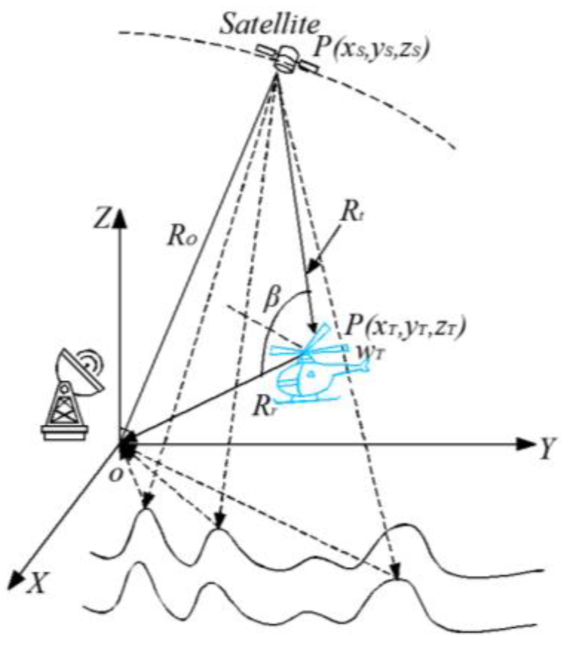
The observation geometry of the GNSS-based PBR system is shown in Figure 1, where the transmitter and receiver are separated. The transmitter is one of the GNSS satellites in the earth orbit, and the receiver is located in origin O of the Cartesian coordinate system. The receiver consists of two channels, namely the reference channel and surveillance channel. and are the transmitter-to-target range and the receiver-to-target range, respectively. is the direct range between the transmitter and receiver. The solid bistatic angle between the helicopter and radar system is defined as .

Figure 1.
PBR geometry with the GNSS illuminator.
To remove the effect of the satellite motion, the Doppler frequency from the satellite motion can be estimated and compensated during the signal capture procedure, and the concrete procedure can be seen in [1]. After this, the transmitter of the bistatic radar can be regarded as fixed. As shown in Figure 1, not only does the surveillance channel acquire the target echo, but also the ground clutter and noise. The principal transmitted signal from the GNSS satellite is a code division multiple access (CDMA) code consisting of pseudo-random noise (PRN).
Of course, any known GNSS signal can be the signal basis for this PBR detection model. For clarity, this paper mainly concentrates on the Global Positioning System (GPS) L1 signal at 1.5 GHz, and the period of the continuous wave is 1 ms. In this space, the Tp = 1ms echo signal is intercepted as a whole for processing. Therefore, the continuous wave signal is modelled as the approximate pulse signal with a pulse width of Tp and pulse repetition frequency of prf = 1/Tp = 1 kHz [18]. The transmitted signal is set as s(t) and the sampled surveillance signal can be written as:
where n and m denote the intercepted fast-time and slow-time domains, respectively; denotes the target echo, which is weaker than the white Gaussian noise ; is the ground clutter:
where , c, and denote the reflectivity, light velocity, and wavelength, respectively. Here, denotes the bistatic range of the ground clutter; represents the envelope function after the match filter. Because there is no relative motion between the ground and radar, the is not varied from the slow-time domain. However, the amplitude of the ground clutter is the strongest in these three parts. Therefore, before the mD feature extraction, the ground clutter needs to be removed from the surveillance channel. One type of mD analysis method adapted to low signal-to-noise ratios (SNRs) has great significance.
According to the target model, the target echo can be modelled as:
where , are the reflectivity and bistatic-range of the ith scatterer within the target.
The direct signal from reference channel can be modelled as:
2.2. The Echo Model of the Helicopter in the PBR
2.2.1. The Fuselage Echo
This paper discusses a situation where the helicopter is hovering. Only the rotor is rotating, and the other parts are nearly stationary. At this time, the bistatic range of the scatterers in the fuselage does not vary over time. Therefore, the fuselage echo can be modelled as:
From this, it can be noted that the fuselage echo model is pretty similar to the ground clutter. Especially in the IO of the GNSS, the resolution cell is larger than the fuselage size, which means the whole fuselage echo will appear in one range cell. The fuselage echo can be written as follows:
where denotes the composited scattering coefficient of the fuselage echo.
Because these echoes are all from fixed scatterers, the ground clutter and fuselage echo are both named the fixed clutter in this paper. The fuselage echo can be eliminated together with the ground clutter using the fixed clutter elimination procedure.
2.2.2. The Rotor Echo of The Helicopter
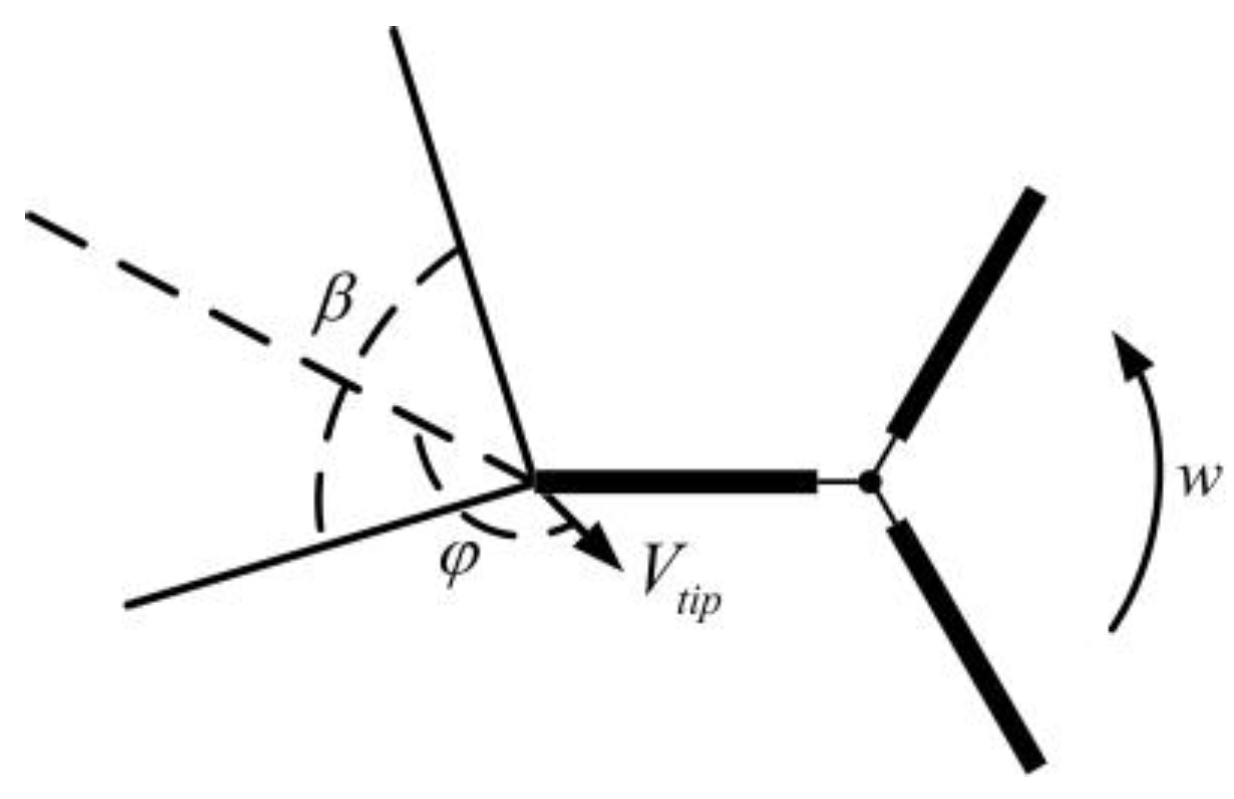
Figure 2 presents a view of the geometry of the rotor blades relative to the bistatic radar. Here, we set the velocity of the blade tip to , with to the angle between and the bisector of the bistatic angle ; denotes the rotation angular frequency and denotes the rotation frequency. For a rigid-body target, the rotation of the rotor blades leads to a variety of bistatic ranges from the slow-time domain m:
where is the bistatic range of the rotation center, is the distance from the ith scatterer to the rotation center, and is the initial rotation angle.

Figure 2.
Micro-motion model.
After integrating the echoes from all scattering points, the rotor echo can be expressed as [19]:
where L is the length of the blade, denotes the amplitude determined by the radar cross-section of the kth blade, and denotes the sinc function. We assume that a rotor consists of K blades that have K different initial angles with .
The mD frequency shift can be obtained for each blade from Equation (9) as:
Owing to the rotation of the rotor, it is obvious that the Doppler frequency is modulated by the sinusoidal function. The maximum mD frequency is:
2.3. Analysis of Flash Generation
Without a loss of generality, from Equation (8), the normalized signal of the first blade is:
It can be seen from Equation (12) that the signal profile includes several sinc peaks; namely, there are several flashes in the slow-time domain. To further analyze the variety of Doppler frequencies, the short-time Fourier transform (STFT) is applied to process the rotor echo. According to the characteristics of the Fourier transform, we know that:
where FT{ } denotes the Fourier transform and ⊗ denotes the convolution operation.
We set the parameters as in Section 4.1, while the TFDs of the profile, the phase, and the entire signal of Equation (13) are shown in Figure 3. Due to the fact that sinc(t) and rect(f) are a Fourier transform pair, Figure 3a shows that there are several flash stripes located at the zero Doppler frequency, which occupies a certain bandwidth. The time width of the stripe is caused by the low time resolution of the STFT. On the other hand, it can be seen from the electromagnetic scattering theorem that the specular reflectivity generates these flashes. From Figure 3b, it is clear that the Doppler frequency is modulated by the sinusoid function, as mentioned above. As described in Equation (13), Figure 3c is the convolution result of Figure 3a,b in the Doppler frequency domain. Instead of being located in the zero-Doppler frequency, the positive frequency flashes centered in the positive frequency and the negative frequency flashes centered in the negative frequency are alternating here.
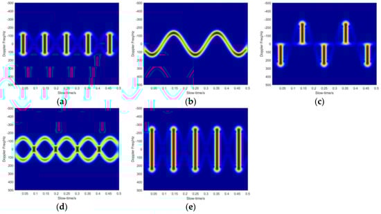
Figure 3.
The STFT of a pair of symmetrical blade signals: (a) the profile, (b) the phase of the asymmetrical rotor, (c) the entire signal of the asymmetrical rotor, (d) the phase of the symmetrical rotor, and (e) the entire signal of the symmetrical rotor.
Furthermore, the mathematical principle for a pair of symmetric blades is similar to that for one blade. The Fourier transform is:
Differing from Equation (13), the phase item of Equation (14) includes a positive phase and a negative phase, as shown in Figure 3d. Hence, the positive frequency flashes and negative frequency flashes appear at the same time in the TFD, as shown in Figure 3e. In short, these flash stripes are produced using the sinc function, but the locations are determined by the echo phase.
3. Clutter Suppression and Micro-Motion Feature Extraction
3.1. Fixed Clutter Suppression Method
3.1.1. The Iteration Elimination
In view of the fact that the clutter (including the direct signal, multipath clutter, and fuselage echo) is much stronger than the rotor echo and noise, the target echo is attributed to noise and the composite approximate noise is constructed. Then, the surveillance signal can be summarized as follows:
where the composite approximate noise is:
Then, the constructed surveillance matrix Ssur can be written as:
where represents the vector of the surveillance echo.
The singular values of the surveillance matrix can respond to the weights of each component. It can be deduced that the larger singular values represent the principal component, while the remaining smaller singular values denote a weak rotor echo and noise. As shown in Equation (15), the surveillance signal is composed of clutter and the composite approximate noise, and the clutter power is greater than the composite noise, meaning the clutter can be regarded as the principal component of the surveillance matrix. The surveillance matrix Ssur can be decomposed to obtain the singular values and related eigenvector matrixes, as shown in Equation (18):
where represents the conjugate transpose. Assuming that the rank (Ssur) = P, then , where denotes all non-zero singular values of the surveillance matrix Ssur and satisfies . According to the singular-value decomposition theorem, the unitary matrix U is composed of all eigenvectors of , and all eigenvectors of form the unitary matrix D. Therefore, the surveillance matrix can be decomposed by:
The first Q larger singular values represent the clutter component, and the clutter suppression can be achieved by eliminating the component relative to the larger singular value from the surveillance matrix Ssur. It is known that the rotor echo power is far lower than the clutter, but the amount of multipath clutter and the number target characteristics are unknown. As a consequence, it is difficult to acquire the number of larger singular values in the initial stage. During concrete processing, the iteration elimination is implemented to remove the clutter, as shown in Equation (20):
where represents the iterations and the initial iteration matrix is set as .
After the matrix decomposition, all singular values are sorted from largest to smallest. The search for the maximum singular value ratio is applied to determine the initial number of iterations , as shown in Equation (21). The proportional coefficient coe is used to give a sufficient iteration allowance, which should be greater than 1.
3.1.2. The Optimal Clutter Elimination Method
Considering that the rotor echo is much lower than the noise, CI is usually implemented to improve the rotor echo power after the clutter suppression. In the processing, two-dimensional pulse compression is implemented to achieve CI. To achieve the optimal clutter elimination effectiveness, the information entropy process is applied to characterize the orderly state or chaos of the CI result, and the mathematical expression is written as in Equation (22). The smaller entropy corresponds to the less and more distinct peaks in the CI results. Firstly, during the ground clutter elimination procedure, the entropy of the CI result is decreased gradually. However, for helicopter target, when the ground clutter is removed completely, the entropy of the CI result begins increasing, since the rotor rotation leads to the sinusoid modulated Doppler frequency, namely the wideband Doppler frequency. There are several peaks in the Doppler frequency domain; hence, the entropy of the CI result will become larger—even larger than the origin. It should be emphasized that this method is applied to suppress the clutter and detect targets. Therefore, the optimal number of iterations is located on the turning point where the entropy of the CI result moves from down to up. The coefficient coe in Equation (21) causes the whole variation process of the entropy.
where En(0) represents the entropy of the CI result of the initial surveillance matrix.
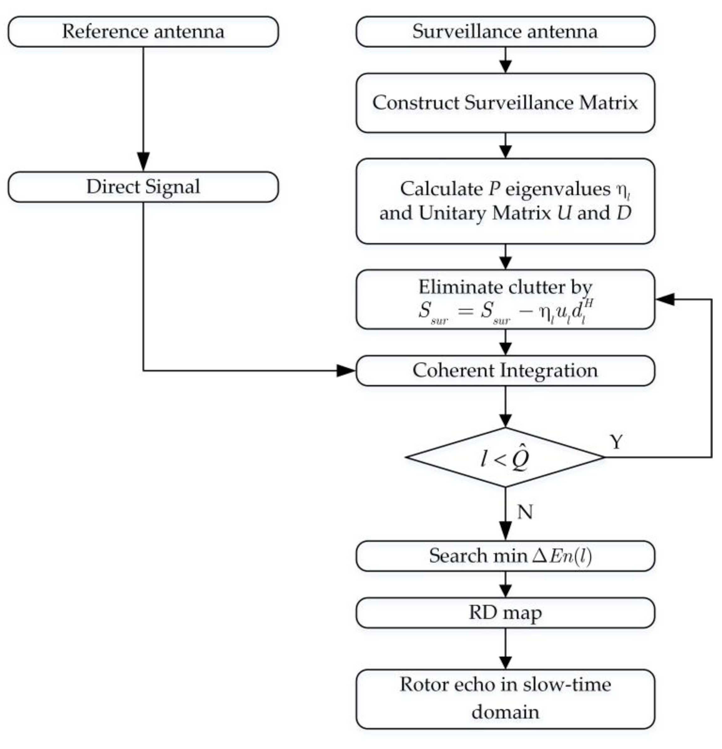
Additionally, the clutter suppression procedure is given in Figure 4.
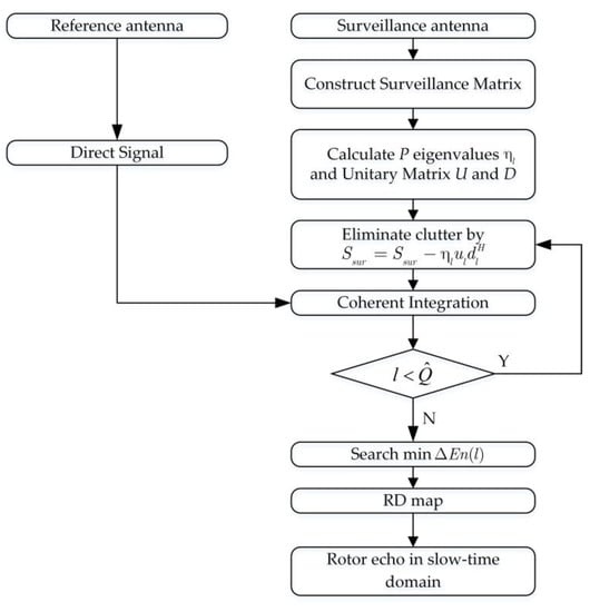
Figure 4.
The clutter suppression procedure.
3.2. Flash Shift in the Time–Frequency Domain
As mentioned in Section 2.3, the variety of flash locations is determined by the sine-function-modulated phase of the rotor echo. In contrast, if the phase of the specific blade echo were compensated completely, those flash stripes of the blade would be centered on a certain Doppler frequency (zero-frequency for an asymmetrical rotor). Next, the analysis of the Doppler center frequency of the flashes is presented.
3.2.1. The Asymmetrical Rotor
The compensation phase is constructed as:
where denote the amplitude, angular frequency, and initial angle, respectively. The problem of parameter estimation is transformed into an optimization problem.
According to Equation (11), we set , and is obtained. Hence, it can be seen that the amplitude is relative to the angular frequency . denotes the bandwidth of the flash stripes, and it can be estimated in the TFD; thus, . Then, the three-dimensional parameter space is decreases to , which can improve the parameter estimation efficiency. Furthermore, the phase-compensated equation (Equation (12)) is:
It can be seen that when and , the phase of Equation (24) is compensated completely and the parameters of the blade are obtained. At the same time, Equation (24) is changed to:
As noted earlier, the TFD of Equation (25) presents a series of flash stripes located in the zero Doppler frequency. In this manner, the flashes of the specific blade are all centered on the zero Doppler frequency after the phase compensation. Then, the rotor blade number K can be obtained directly from the flash number between nearest two zero-frequency flashes in the TFD.
3.2.2. The Symmetrical Rotor
Because of the symmetry of the rotor, each flash of the specific symmetric blade pair, including the positive frequency flash and negative frequency flash, is called a “double flash”. The compensation procedure is as follows:
where denotes the bandwidth of the double flash.
At this time, when and , Equation (26) is changed to:
The phase of the first item is compensated completely in Equation (26); thus, the flashes are all centered on the zero-Doppler frequency. However, the phase of the second item in Equation (26) is changed to the double initial, ignoring the effect of the minus sign. In the second item of Equation (27), the mD frequency is twice the initial value; hence, the flash stripes are centered on or . It can be noted that the two flashes of these two items are connected together, without overlap along the Doppler frequency axis. Then, the composited double flash of the specific symmetrical blade pair can only be centered on or , and these two center frequencies are alternating. As before, all double flashes of the specific symmetrical blade pair after the phase compensation can be sought out by the centered frequency. Then, the number of symmetrical blade pairs can be obtained, and the blade number of the rotor can be obtained.
3.3. Optimization Criterion
The standard frequency (SF) that is the center frequency of the completely compensated flash for the different rotor structure is analyzed in Section 3.2. We found that the blade number of a rotor usually does not exceed 8, meaning the SF dictionary can be constructed as in Table 1.

Table 1.
The standard frequency dictionary.
The horizontal axis represents the standard flashes and their SF, while the vertical axis represents the blade number. For simplicity, the SF of double flash is described as a function of B2. For one blade, every flash is regarded as a standard flash, and the SFs after the TFFS all equal zero. For two blades, all double flashes are identical standard flashes, but the SF alternates between and . For three blades, there are two non-zero-frequency flashes of the other blades between the nearest two standard flashes , and the SFs are all zero. As for other cases, the distributions of the standard flashes and the SFs are shown in Table 1.
To obtain the optimal compensation result, the center frequencies of all standard flashes are compared with the SF dictionary . The mean l1 norm for the parameter space is:
where k denotes the blades number in the dictionary, I denotes the number of standard flashes, and | | denotes the l1 norm. Since is a matrix that has the same dimensions as the parameter space for each k, it is a three-dimensional matrix.
Then, the blade number and can be obtained by searching for the minimum of from the parameter space . Finally, the blade length can be calculated as:
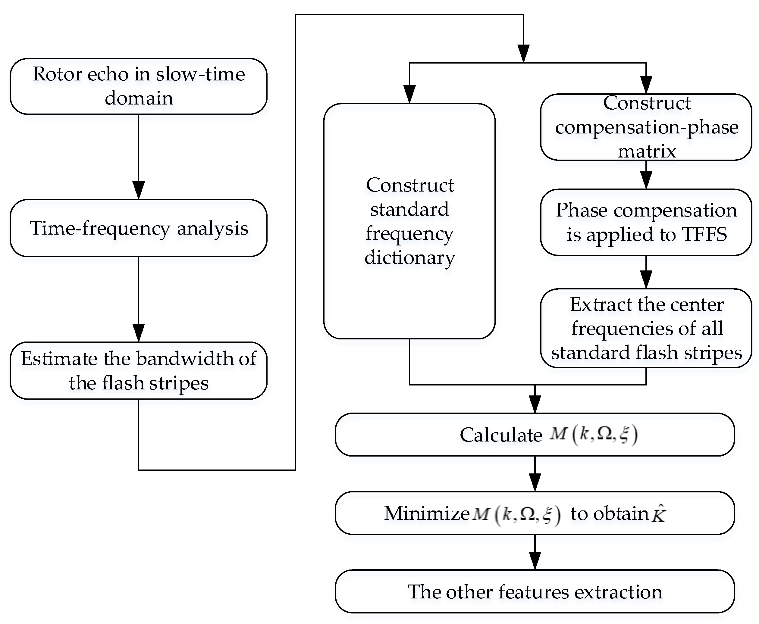
Additionally, the flowchart of the proposed mD feature extraction method is given in Figure 5.
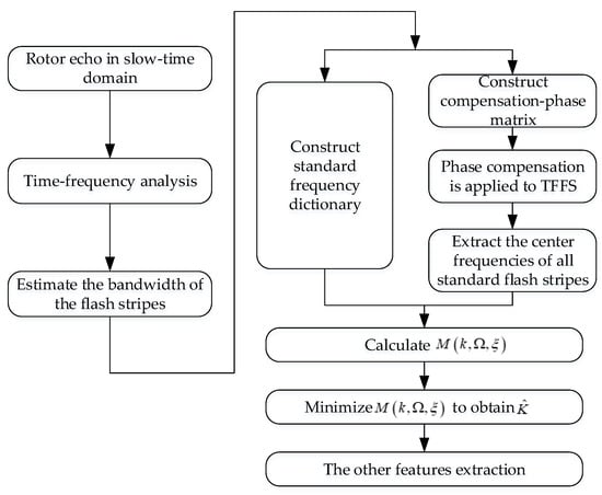
Figure 5.
The flowchart of the proposed method.
4. Simulation Experiments
4.1. The Scattering Point Model Simulation Experiments
To demonstrate the effectiveness of the proposed method, a helicopter was modelled for the GPS-based bistatic radar. After the satellite motion compensation phase during signal capture, the GPS satellite is regarded as stationary. The surveillance channel consists of the target echo, direct signal, and five paths of ground clutter, and the ground clutter parameters are shown in Table 2. The helicopter is a model of a fuselage and rotor; the fuselage is modelled as uniform scatters and the rotor is modelled as three blades with a length L = 7.3 m, as well as a perfect electrical conductor. The blades are assumed to rotate at a rotation frequency fr = 4.8 r/s and to be illuminated by a simulated GPS L1 signal in the location where the bistatic factor , as shown in Figure 1. The sampling rate of the employed receiver is set to 2.046 MHz. Finally, the simulation experiments are implemented under SNR = −25 dB, namely the SNR of the raw helicopter target echo before the CI is −25 dB.
Table 2.
The simulation parameters.
4.1.1. The Clutter Suppression
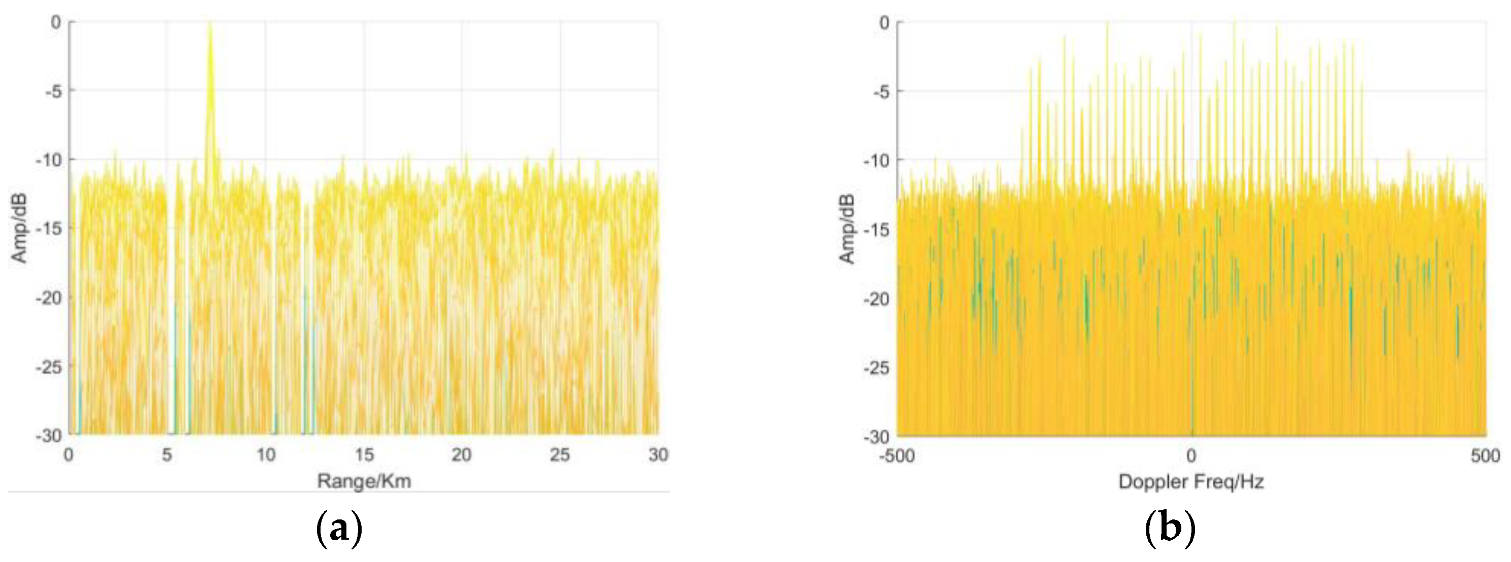
After sampling signal, the raw surveillance signal is constructed as a surveillance matrix, and the CI result of the surveillance matrix is shown in Figure 6. It is obvious that there is a strong peak indicating the direct signal in (0.4399 Km, 0.6676 Hz). For the sake of observation, the direct signal is shifted in the bi-range of 0.4399 Km in this simulation experiment. The Doppler frequency of the direct signal would be zero after the signal capture and satellite motion compensation phases, but the spectrum leakage brings the Doppler frequency to 0.6676 Hz. From this, it is known that only the direct signal can be detected from the CI result for the raw surveillance matrix, and the rotor echoes are submerged in strong cluttering and noise. Therefore, the clutter suppression is necessary before the micro-motion feature extraction.
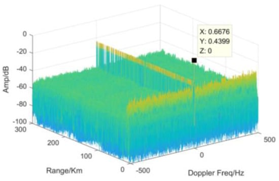
Figure 6.
The CI of raw echoes.
Next, the raw surveillance matrix is processed using the proposed iteration elimination method. Firstly, the singular decomposition phase is implemented, and the change in the singular value ratio is shown in Figure 7. For a clearer view, only the first 50 singular ratio values are shown here. From the image, it is clear that the singular value ratio presents a procedure of increasing and then decreasing, so the inflection point is the focus. The 7th singular ratio value is the maximum, which means that the variation between the 7th and the 8th singular values is the most dramatic. Namely, the first seven larger singular values denote the strong clutter component that needs to be eliminated, and the other smaller singular values indicate the rotor echo component and noise. For enough iteration margin, the factor coe is set to 2 in this experiment, and then the initial iterations can be set to 14.
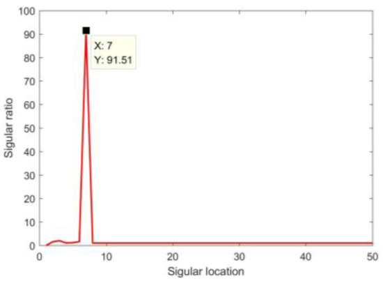
Figure 7.
The singular ratio distribution.
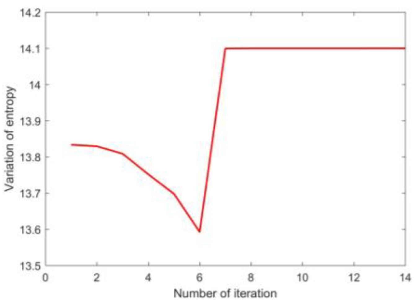
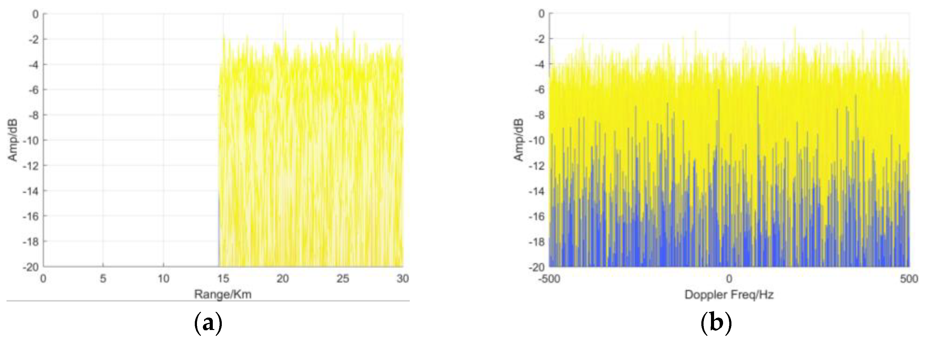
As mentioned above, the strong clutter will be eliminated by the iterations. The optimal number of iterations is determined by the entropy variation of the CI results, and the entropy variation during the iterations in the experiment is shown in Figure 8. It can be seen that entropy variation presents a decreasing and then increasing trend with the increase in iterations. From the 1st to 6th iterations, the entropy is decreasing gradually, then the entropy reaches the minimum at the 6th iteration. The reason is that the fixed clutter is eliminated gradually during this process, whereby the clutter peaks are cut down. After 7 iterations, the fixed clutter is removed completely, and the surveillance signal only includes the rotor echo. Differing from the normal motion target, the rotor includes several rotating blades. The Doppler frequency of the rotor echo is modulated by the sinusoid function, and there are several peaks in the Doppler frequency domain after the CI. Hence, the entropy of the CI results of the rotor echo is much larger. However, the rotor echo also fades gradually after 8 iterations. Because the rotor consists of many scatterers, the first several iterations will not have an evident impact on the CI result, and the entropy remains nearly constant after the 7th iteration. To guarantee the integrity of the rotor echo, the optimal number of iterations is selected as 7. Then, the clutter-suppressed surveillance matrix is processed via CI, and the result is shown in Figure 9. There is a peak at about 7 Km that denotes the rotor echo in Figure 9a, and the strong clutter at 0.4399 Km is removed. Figure 9b indicates the Doppler frequency–amplitude plane of the CI result, where the rotor echo occupies a certain bandwidth. As discussed above, the wideband signal is produced by the rotational rotor. Therefore, after clutter suppression, the helicopter or the rotor can be detected and the rotor echo in the slow-time domain can be obtained.

Figure 8.
The entropy variation during successive iterations.

Figure 9.
The CI after iteration elimination: (a) the range–amplitude plane; (b) the Doppler frequency–amplitude plane.
To illustrate the effectiveness of the clutter elimination method proposed in this paper, the detection property is compared with the ECA. Firstly, each pulse is processed using the ECA with the direct signal. Then, the CI result is shown in Figure 10. The bi-range of the target is 7.24 Km, but the bi-range of multipath 2 exceeds 12 Km. Accordingly, the ECA is applied to suppress the fixed clutter within 15 Km in this experiment. From Figure 10a, it can be seen that the fixed clutter within 15 Km is suppressed entirely. Figure 10b shows the Doppler frequency–amplitude plane, although there is no wideband spectral illustration as in Figure 9b. It is obvious that the whole rotor echo is also removed. The ECA cannot be used for helicopter detection in this experiment.

Figure 10.
The CI after the ECA: (a) the range–amplitude plane; (b) the Doppler frequency–amplitude plane.
In brief, the ECA has an intrinsic limitation. Because the ECA achieves target detection by removing the short bi-range ground clutter, the ECA cannot achieve helicopter target detection when the bi-range of the target is smaller than that of the clutter. However, the proposed iteration elimination method is aimed at the echo energy, meaning it has a better effect.
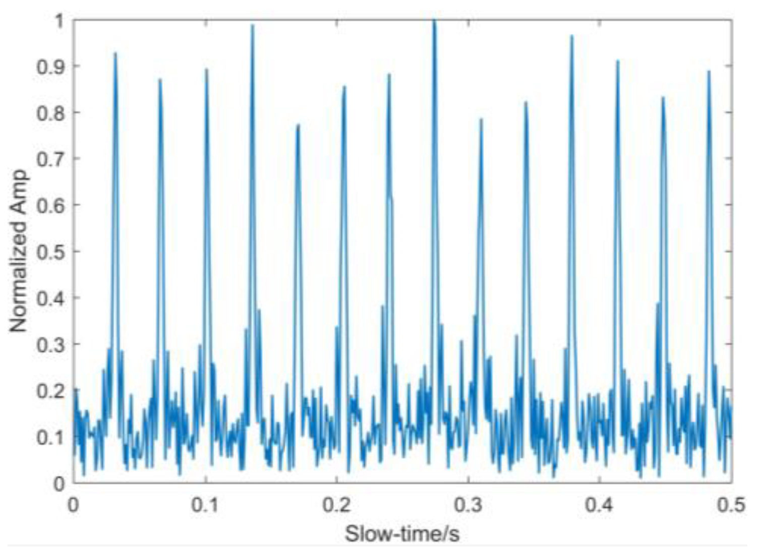
4.1.2. The Micro-Motion Feature Extraction
After the fixed clutter suppression, the rotor echo in the slow-time domain can be extracted from the clutter-suppressed surveillance matrix. Figure 11 gives the range profile for this, which shows that the rotor echo mainly consists of several sinc peaks, as described in Section 2.2. In other words, there are several iterations of specular reflection between the target and bistatic radar. For a further analysis, Figure 12 presents the TFD of the extracted rotor echo by utilizing the STFT. It is different from Figure 11 in that there are alternating positive flashes and negative flashes in the TFD. The bandwidth B1 of each flash is about 286.6 Hz. As discussed above, the asymmetry of the flashes in the TFD is caused by the asymmetry of the rotor. Therefore, it can be seen that the rotor is comprised of odd blades. The dimension of the SF dictionary is decreased to four (1, 3, 5, 7). The concrete dictionary for this experiment is shown in Table 3. From this, the different standard flashes are utilized for the different blade numbers.

Figure 11.
The range profiles.
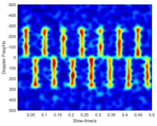
Figure 12.
The TFD of the raw echo.
Table 3.
The standard frequency dictionary in this experiment.
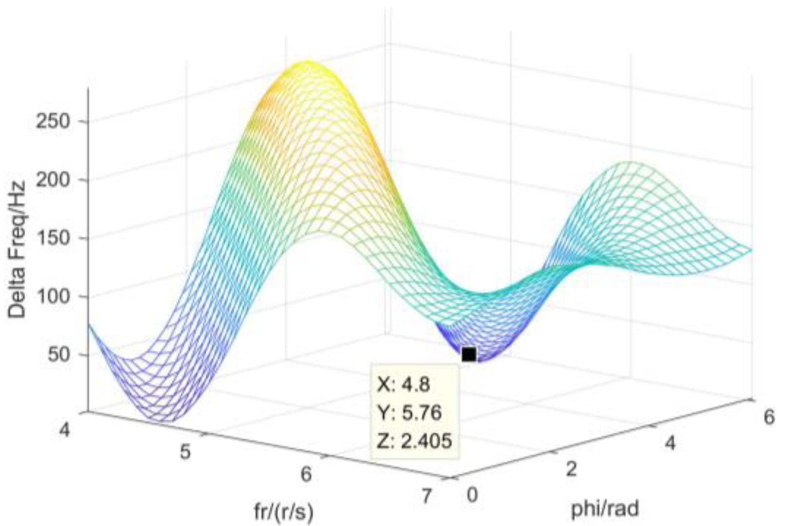
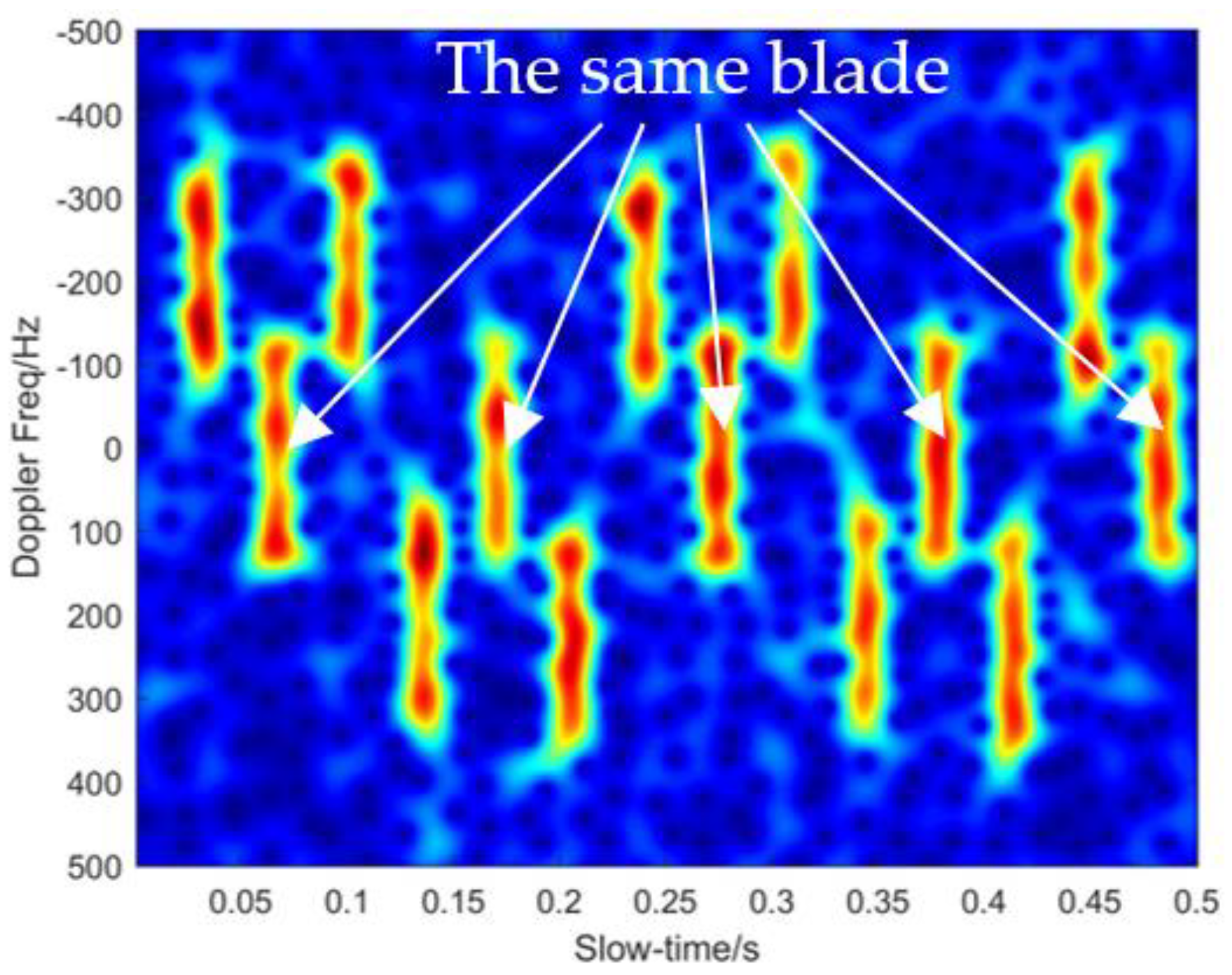
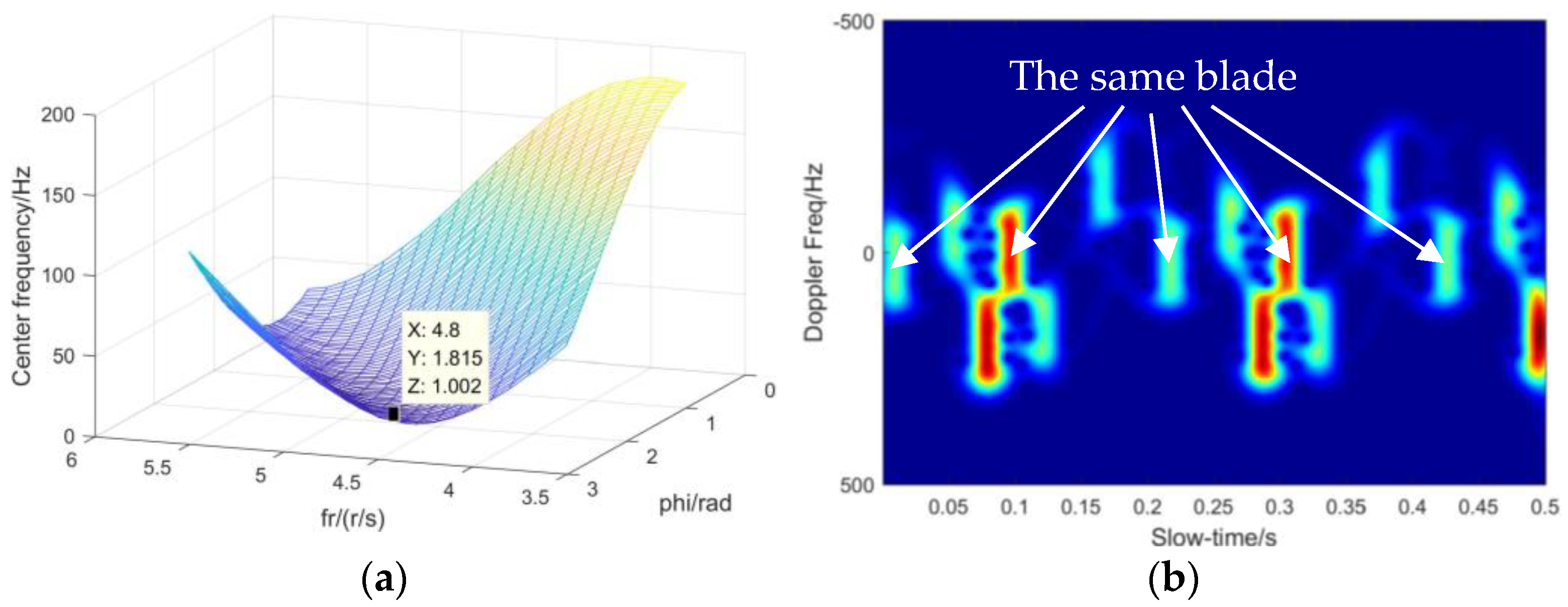
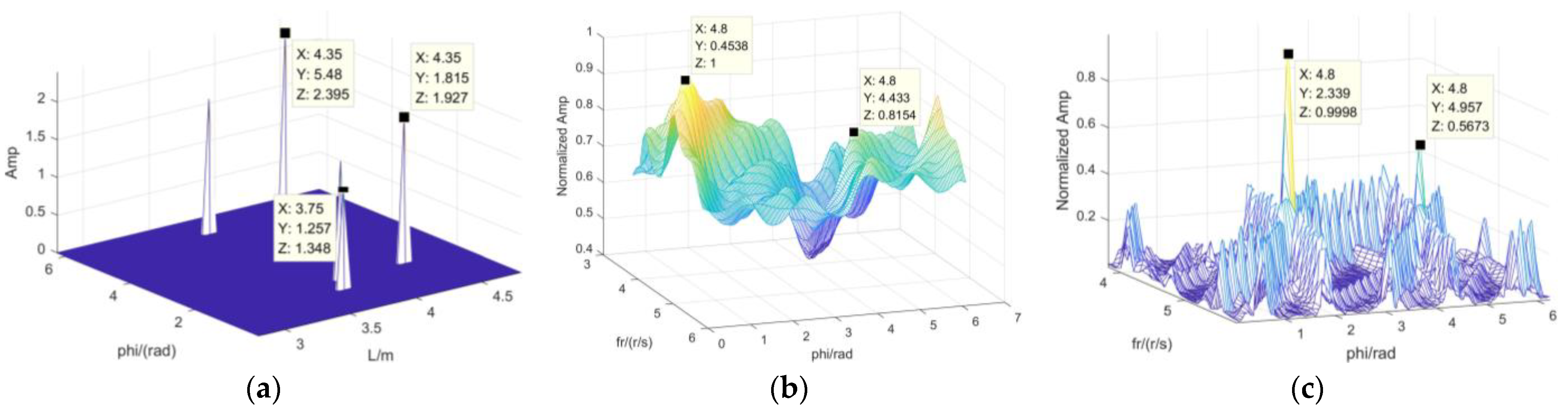
Figure 13 presents the minimum values for different blade numbers k (1, 3, 5, 7). In this image, a minimum can be found when K = 3, which means the rotor consists of 3 blades. The variety of values is given in Figure 14. As presented in Section 3.3, the is the same dimensional matrix as the parameter space. From the image, it is obvious that reaches the minimum value 2.405 when r/s and . Based on the estimated parameters, the length of the blades can be calculated as in Equation (29), and . Otherwise, the TFD after the complete phase compensation procedure is as shown in Figure 15. There are a series of flashes centering on the zero frequency, as illustrated by the white arrows, which belong to the same blade. It can be seen that there are two non-zero-frequency flashes from other blades between the nearest two zero-frequency flashes, and consequently the rotor structure includes 3 blades. The result from Figure 15 is coincident with that of . The above coincident estimation results demonstrate the effectiveness of the proposed method.
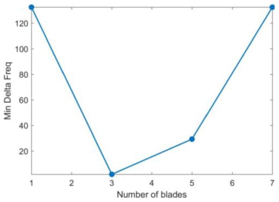
Figure 13.
The variety of delta frequency values from k.
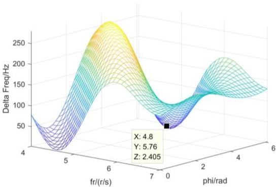
Figure 14.
The variety of values.
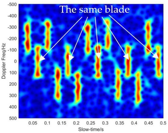
Figure 15.
The optimal shifted TFD.
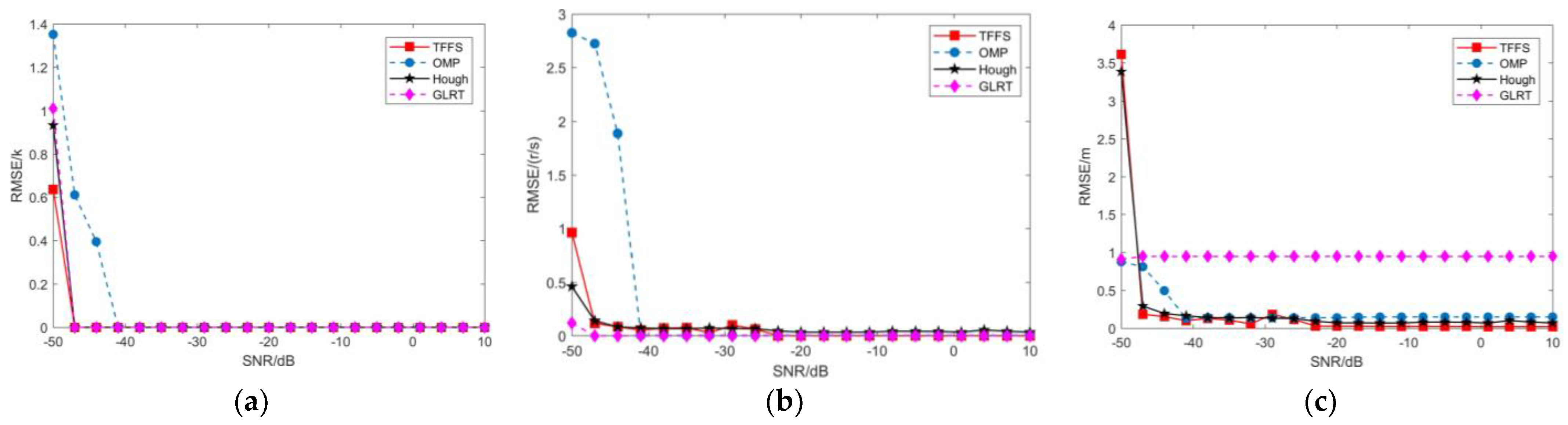
In order to validate the anti-noise ability of the proposed method, 100-iteration Monte Carlo simulation experiments are conducted, and Figure 16 gives the root mean square errors (RMSEs) of the estimated parameters with the increasing SNRs. In Figure 16, the simulation parameters are the same as above, but the SNR increases from −50 dB to 10 dB with the step size of 3 dB. For comparison, the processing results for the classic OMP, Hough transform, and GLRT algorithm are also presented.
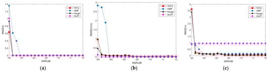
Figure 16.
The parameters estimation RMSEs: (a) estimation RMSE of K; (b) estimation RMSE of fr; (c) estimation RMSE of L.
Firstly, it can be seen from Figure 16a that these four methods can all obtain accurate the blade number for the rotors when the SNR is greater than −40 dB. Even the TFFS, HT, and GLRT methods can obtain the correct blade number when the SNR is as low as −47 dB. However, Figure 16a illustrates that the OMP algorithm cannot obtain the true blade number when the SNR is smaller than −40 dB. Accordingly, the proposed TFFS algorithm is more robust than the OMP algorithm at low SNRs. Figure 16b,c show the RMSEs of the rotation frequency and blade length, respectively, with increasing SNRs. In Figure 16b, it is obvious that the purple diamond broken curve is lower than other three curves for all SNRs. The rotation frequency RMSEs of the TFFS and HT methods are pretty close. These three estimation results are nearly identical when the SNR is greater than −20 dB. It is believed that the estimation results for the GLRT are slightly better than the HT and the proposed TFFS method for the rotation frequency is better at low SNRs. Figure 16c shows that the red square line is lower than other three curves, and the purple diamond broken line is close to 1 m. Therefore, it is agreed that the proposed TFFS method can obtain accurate blade length values, but the blade length RMSE of the GLRT method is greater. The main reason is the effect of the flashes in the slow-time domain, whereby the GRLT cannot estimate the true blade length. Overall, the proposed TFFS algorithm can accurately extract the mD feature, and it is more robust than the classic OMP, HT, and GLRT algorithms.
4.2. The PO Facet Model Experiments
To validate the effectiveness of the proposed mD feature extraction method, the TFFS method is tested using the electromagnetic calculation data. Hence, this experiment assumes that the fixed clutter has been eliminated. The physical optics (PO) method is applied to generate the rotor echoes in the bistatic radar, and this experiment will consider the shield and rebound of the electromagnetic wave. Therefore, the PO facet model is designed to simulate the work situation of the real passive bistatic radar.
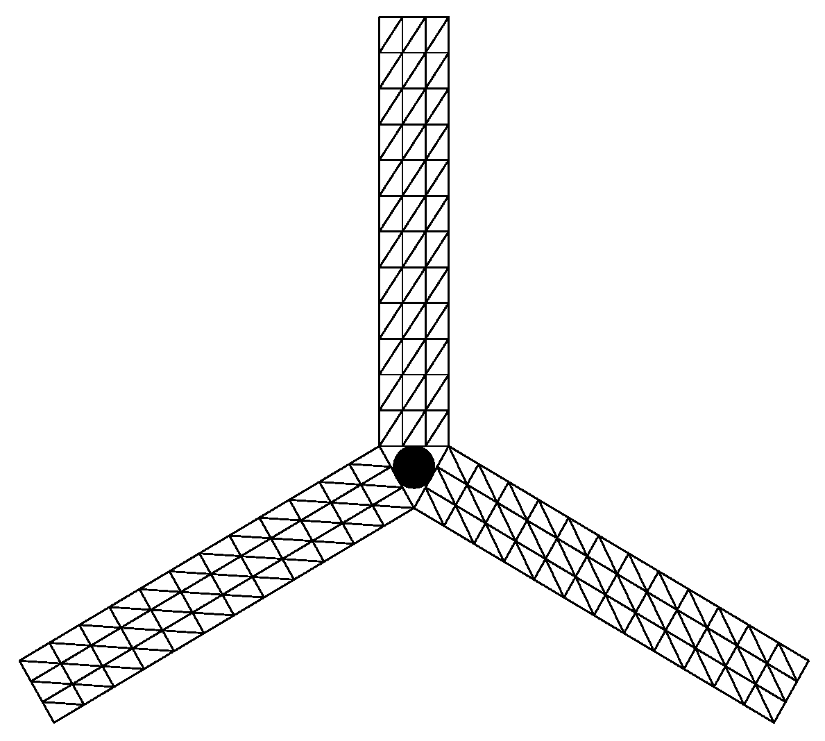
Based on the PO facet radar cross-section model, a rotor model can be represented by the arrays of triangular facets. The scatterer center of each triangle is assumed to be the geometric centroid of its triangle vertices, and the simulated three-blade rotor model is shown in Figure 17. The bistatic angle of the simulated model is 150°, which is the sum of 70° (incident elevation angle) and 80° (reception elevation angle). The larger size of the rotor will lead to greater calculation complexity. To reduce the calculation complexity, the length and width of the target are changed to 3.9 m and 0.2 m, respectively, and the carrier frequency is also 1.5 GHz.
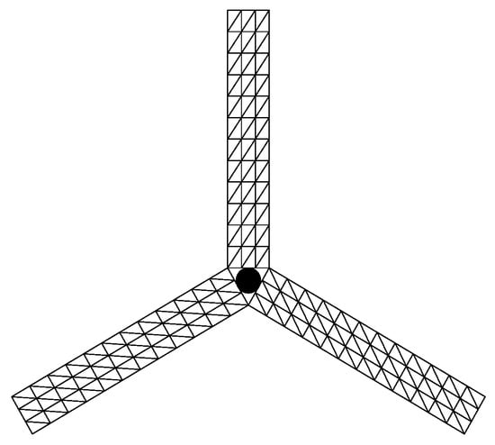
Figure 17.
PO facet model of a simulated three-blade rotor.
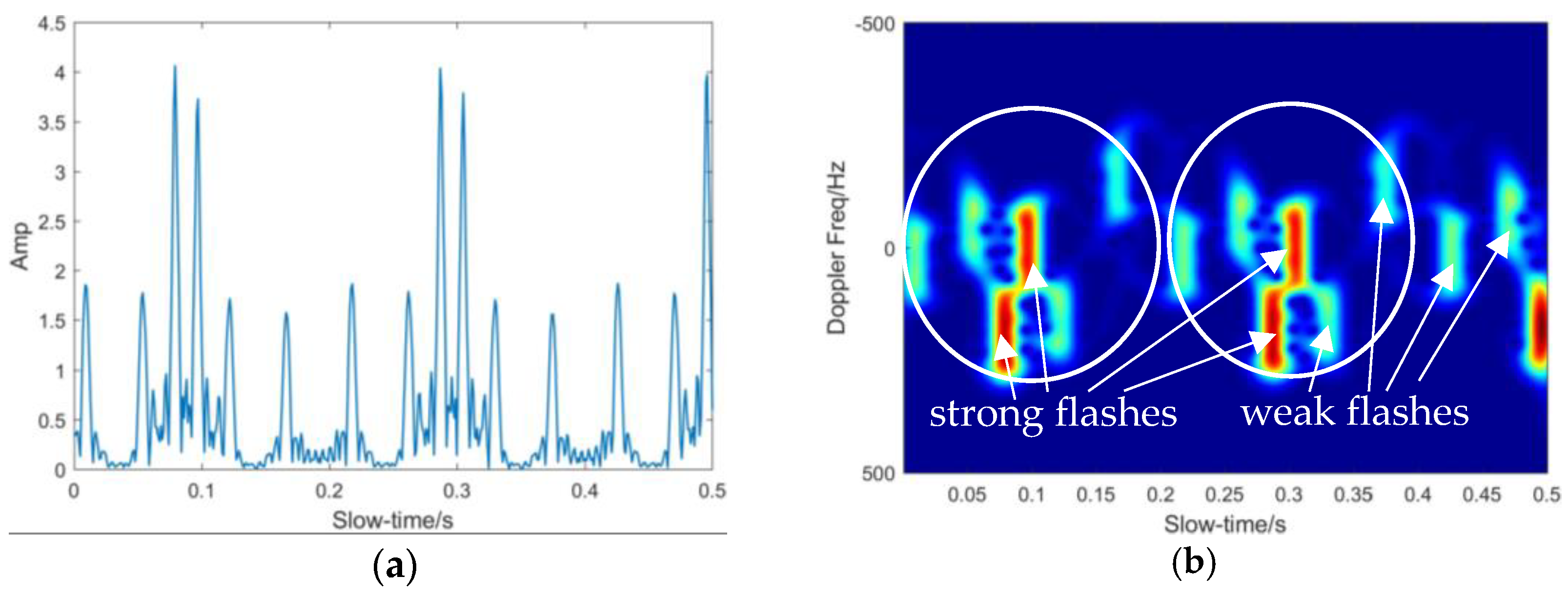
Figure 18 presents the simulated echo from the PO electromagnetic calculation method. Differing from the scattering point model, the scatter intensity of the peak varies severely from the slow-time domain in Figure 18a. The reason is that the scatter intensity varies in different parts in the rotor. Otherwise, as a result of the incline of the observation model, the peak intervals are also not homogeneous. In the TFD, it can be seen that the flash intensity and interval are also varied, as presented in Figure 18b. A closer observation can reveal that the six flashes can be regarded as a rotation cycle that includes two strong flashes and four weak flashes, as indicated in the white circle in Figure 18b. The processing results of the proposed TFFS method are given in Figure 19. Figure 19a demonstrates that the estimated rotation frequency is 4.8 r/s. Furthermore, the blade length can be obtained as written in Table 4. The optimal TFD after the TFFS processing is shown in Figure 19b. As indicated in Figure 19b, the white arrow marks the zero-frequency flashes belonging to the same blade. It is obvious that there are two non-zero-frequency flashes from other blades between the nearest two zero-frequency flashes. Therefore, it can be concluded that the rotor consists of three blades. Furthermore, the strength of the nearest two zero-frequency flashes shows a great change. The reason is that the reflectivity values of the blade moving toward and that of the same blade going away are not identical in the bistatic radar.

Figure 18.
The simulated PO echoes: (a) the range profile of the PO echoes; (b) the TFD of the original echoes.

Figure 19.
The processing result of the TFFS: (a) parameter estimation results of the TFFS; (b) the optimal shifted TFD.
Table 4.
The estimation results for the methods in the PO facet simulation model.
For comparison, the processing results for the OMP, HT, and GLRT methods are also given in Figure 20, and the parameter estimation results are all written in Table 4. It can be seen that there are several sidelobes around the three main lobes in Figure 20a. In addition, the sidelobes and main lobe are almost located at an identical blade length or initial angle. Thus, we can ignore these sidelobes and only consider the three main lobes in the OMP parameter estimation results. The rotor consists of three blades. Only two obvious peaks have stronger reflectivity values that can be observed in Figure 20b; namely, the HT method processing result only detects two blades, and the rotation frequency is about 4.8 r/s. Additionally, the processing result for the GLRT method also includes two strong peaks, as shown in Figure 20c. In other words, the GLRT method only detects two blades of the rotor. The principal reason for the worse processing results is the inhomogeneous nature of the scatter intensity. According to Table 4, only the proposed TFFS and OMP methods can detect the three blades of the rotor, and the estimation result of the TFFS method is more accurate than that of the OMP method.

Figure 20.
Processing results for the OMP, HT, and GLRT methods: (a) OMP method; (b) HT method; (c) GLRT method.
With these classic methods, the number of peaks in the parameter search result determines the blade number. The inhomogeneous reflectivity of the rotor can generate the different acuity peaks; hence, the acuity of the peaks can also affect the parameter estimation accuracy. However, the parameter search result for the proposed method only includes one valley, and the blade number can be obtained from the optimal TFD directly. Consequently, in the PO facet model simulation experiments, the proposed TFFS can also obtain more accurate parameter estimation results.
5. Conclusions
Focusing on the micro-motion feature extraction process for the GNSS-based PBR, this paper proposed a fixed clutter suppression method based on iteration elimination and a feature extraction method based on the TFFS method for a helicopter rotor. In the proposed method, the SVD is utilized to disassemble the clutter component and the rotor echo component in the surveillance signal, and the iterations of the clutter component corresponding to the larger singular values are eliminated gradually. In comparison to the ECA, the iteration elimination method can be sued for helicopter detection and rotor echo extraction when the bi-range of the target is shorter than that of the clutter. Next, the TFFS algorithm was applied to shift the standard flashes to a certain frequency. Then, the feature parameters of the rotor were extracted by minimizing the mean l1 norm . Finally, the scattering point model and PO facet model simulation experiments were performed to validate the effectiveness and robustness of the new method. Compared with the classic OMP, HT, and GLRT methods, this method can achieve more accurate and robust rotor feature extraction results for a helicopter.
Author Contributions
Conceptualization, S.X.; Data curation, J.L.; Formal analysis, Z.Z.; Investigation, Z.W. and B.W.; Writing—original draft, Z.Z. All authors have read and agreed to the published version of the manuscript.
Funding
This research received no external funding.
Conflicts of Interest
The authors declare no conflict of interest.
References
- Zuo, R. Bistatic Synthetic Aperture Radar Using GNSS as Transmitters of Opportunity. Ph.D. Thesis, The University of Birmingham, Birmingham, UK, 2012. [Google Scholar]
- Pui, C.Y. Large Scale Antenna Array for GPS Bistatic Radar. Ph.D. Thesis, The University of Adelaide, Adelaide, Australia, 2017. [Google Scholar]
- Pastina, D.; Santi, F.; Pieralice, F.; Bucciarelli, M.; Ma, H.; Tzagkas, D.; Antoniou, M.; Cherniakov, M. Maritime Moving Target Long Time Integration for GNSS-Based Passive Bistatic Radar. IEEE Trans. Aerosp. Electron. Syst. 2018, 54, 3060–3083. [Google Scholar] [CrossRef]
- Gang, C.; Jun, W.; Luo, Z.; Zhao, D.; Wen, Y. Two-stage clutter and interference cancellation method in passive bistatic radar. IET Signal Process. 2020, 14, 342–351. [Google Scholar] [CrossRef]
- Hu, C.; Liu, C.; Wang, R.; Chen, L.; Wang, L. Detection and SISAR Imaging of Aircrafts Using GNSS Forward Scatter Radar: Signal Modeling and Experimental Validation. IEEE Trans. Aerosp. Electron. Syst. 2017, 53, 2077–2093. [Google Scholar] [CrossRef]
- Steigenberger, P.; Thoelert, S.; Montenbruck, O. GNSS Satellite Transmit Power and its Impact on Orbit Determination. J. Geod. 2017, 92, 609–624. [Google Scholar] [CrossRef]
- Baczyk, M.K.; Samczynski, P.; Kulpa, K.; Misiurewicz, J. Micro-Doppler signatures of helicopters in multistatic passive radars. IET Radar Sonar Navig. 2015, 9, 1276–1283. [Google Scholar] [CrossRef]
- Gong, J.; Yan, J.; Li, D.; Chen, R.; Tian, F.; Yan, Z. Theoretical and experimental analysis of radar micro-Doppler signature modulated by rotating blades of drones. IEEE Antennas Wirel. Propag. Lett. 2020, 19, 1659–1663. [Google Scholar] [CrossRef]
- Nakamura, R.; Hadama, H. Characteristics of ultra-wideband radar echoes from a drone. IEICE Commun. Express 2017, 6, 530–534. [Google Scholar] [CrossRef]
- Antoniou, M.; Hong, Z.; Zeng, Z.; Zuo, R.; Zhang, Q.; Cherniakov, M. Passive bistatic synthetic aperture radar imaging with Galileo transmitters and a moving receiver: Experimental demonstration. IET Radar Sonar Navig. 2013, 7, 985–993. [Google Scholar] [CrossRef]
- Tabassum, M.N.; Hadi, M.A.; Alshebeili, S. CS based processing for high resolution GSM passive bistatic radar. In Proceedings of the 2016 IEEE International Conference on Acoustics, Speech and Signal Processing (ICASSP), Shanghai, China, 20–25 March 2016; pp. 2229–2233. [Google Scholar]
- Cardinali, R.; Colone, F.; Ferretti, C.; Lombardo, P. Comparison of Clutter and Multipath Cancellation Techniques for Passive Radar. In Proceedings of the 2007 IEEE Radar Conference, Waltham, MA, USA, 17–20 April 2007. [Google Scholar]
- He, Z.-Y.; Yang, Y.; Wu, C.; Weng, D.J. Moving Target Imaging Using GNSS-Based Passive Bistatic Synthetic Aperture Radar. Remote Sens. 2020, 12, 3356. [Google Scholar] [CrossRef]
- Colone, F.; O’Hagan, D.W.; Lombardo, P.; Baker, C.J. A Multistage Processing Algorithm for Disturbance Removal and Target Detection in Passive Bistatic Radar. IEEE Trans. Aerosp. Electron. Syst. 2009, 45, 698–722. [Google Scholar] [CrossRef]
- Bi, W.; Zhao, Y.; An, C.; Hu, S. Clutter Elimination and Random-Noise Denoising of GPR Signals Using an SVD Method Based on the Hankel Matrix in the Local Frequency Domain. Sensors 2018, 18, 3422. [Google Scholar] [CrossRef] [PubMed]
- Kumar, S.; Kumar, S.G. Parameter Estimation of Frequency Modulated Continuous Wave (FMCW) Radar Signal Using Wigner-Ville Distribution and Radon Transform. Int. J. Adv. Res. Comput. Commun. Eng. 2014, 3. [Google Scholar]
- Gong, J.; Yan, J.; Li, D. Comparison of micro-Doppler signatures registered using RBM of helicopters and WSM of vehicles. IET Radar Sonar Navig. 2019, 13, 1951–1955. [Google Scholar] [CrossRef]
- Addabbo, P.; Clement, C.; Ullo, S.L. Fourier independent component analysis of radar micro-Doppler feature. In Proceedings of the 2017 IEEE International Workshop on Metrology for AeroSpace (MetroAeroSpace), Padua, Italy, 21–23 June 2017; pp. 45–49. [Google Scholar]
- Clemente, C.; Soraghan, J.J. GNSS-Based Passive Bistatic Radar for Micro-Doppler Analysis of Helicopter Rotor Blades. IEEE Trans. Aerosp. Electron. Syst. 2014, 50, 491–500. [Google Scholar] [CrossRef]
- Wang, W.; Tang, Z.; Chen, Y.; Sung, Y. Parity recognition of blade number and maneuver intention classification algorithm of rotor target based on micro-Doppler features using CNN. J. Syst. Eng. Electron. 2020, 31, 884–889. [Google Scholar]
- Singh, A.K.; Kim, Y.H. Accurate measurement of drone’s blade length and rotation rate using pattern analysis with W-band radar. Electron. Lett. 2018, 54, 523–525. [Google Scholar] [CrossRef]
- Zhang, W.; Li, G.; Baker, C. Radar Recognition of Multiple Micro-Drones Based on Their Micro-Doppler Signatures via Dictionary Learning. IET Radar Sonar Navig. 2020, 14, 1310–1318. [Google Scholar] [CrossRef]
- Tran, H.T.; Heading, E.; Melino, R. OMP-based translational motion estimation for a rotating target by narrowband radar. IET Radar Sonar Navig. 2017, 11, 854–860. [Google Scholar] [CrossRef]
- Chen, V.C.; Tahmoush, D.; Miceli, W.J. Radar Micro-Doppler Signature Processing and Applications; The 505 Institution of Engineering and Technology: London, UK, 2014; pp. 187–227.
- Deng, B.; Wang, H.Q.; Li, X.; Qin, Y.L.; Wang, J.T. Generalised likelihood ratio test detector for micro motion targets in synthetic aperture radar raw signals. IET Radar Sonar Navig. 2011, 5, 528–535. [Google Scholar] [CrossRef]
- Oh, B.S.; Guo, X.; Wan, F.; Toh, K.A.; Lin, Z. Micro-Doppler Mini-UAV Classification Using Empirical-Mode Decomposition Features. IEEE Geoence Remote Sens. Lett. 2017, 15, 227–231. [Google Scholar] [CrossRef]
- Melino, R.; Kodituwakku, S.; Tran, H.T. Orthogonal matching pursuit and matched filter techniques for the imaging of rotating blades. In Proceedings of the 2015 IEEE Radar Conference, Johannesburg, South Africa, 27–30 October 2015. [Google Scholar]
- Fang, X.; Xiao, G.Q. Rotor Blades Micro-Doppler Feature Analysis and Extraction of Small Unmanned Rotorcraft. IEEE Sens. J. 2020, 21, 3592–3601. [Google Scholar] [CrossRef]
- Wu, J.; Zuo, L.; Li, M. Micro-Doppler of helicopter with different blade shapes. Electron. Lett. 2018, 54, 1053–1054. [Google Scholar] [CrossRef]
- Choi, I.; Kang, K.-B.; Jung, J.H.; Park, S.H. Efficient Estimation of the Helicopter Blade Parameter by Independent Component Analysis. IEEE Access 2020, 8, 156889–156899. [Google Scholar] [CrossRef]


Publisher’s Note: MDPI stays neutral with regard to jurisdictional claims in published maps and institutional affiliations. |
© 2022 by the authors. Licensee MDPI, Basel, Switzerland. This article is an open access article distributed under the terms and conditions of the Creative Commons Attribution (CC BY) license (https://creativecommons.org/licenses/by/4.0/).