Impact of Lidar Data Assimilation on Simulating Afternoon Thunderstorms near Pingtung Airport, Taiwan: A Case Study

Abstract

This study focused on improving the forecasting of the afternoon thunderstorm (AT) event on 5 August 2018 near Pingtung Airport in southern Taiwan through a three-dimensional variational data assimilation system using Doppler lidar-based wind profiler data from the Weather and Research Forecast model. The assimilation of lidar wind profiler data had a positive impact on predicting the occurrence and development of ATs and wind fields associated with the local circulations of the sea–land breeze and the mountains. Evaluation of the model quantitative precipitation forecast by using root-mean-square error analysis, Pearson product–moment correlation coefficient analysis, Spearman rank correlation coefficient analysis, and threat and bias scores revealed that experiments using data assimilation performed much better than those not using data assimilation. Among the experiments using data assimilation, when the implementation time of assimilation of the wind profiler data in the model was closer to the occurrence time of the observed ATs, the forecast performance greatly improved. Overall, our assimilation strategy has crucial implications for the prediction of short-duration intense rainfall caused by ATs with small temporal and spatial scales of few hours and a few tens of kilometers. Our strategy can help guarantee the flight safety of aircraft.

1. Introduction

Afternoon thunderstorms (ATs), which feature short-duration intense rainfall, typically develop in summer when the sun heats the air near the ground [1,2]. Compared with mesoscale convective systems such as squall lines, cold fronts, and tropical cyclones, ATs have smaller scales of space and time [3]. Taiwan, with a total land area of 36,000 km², is an island with a warm and humid climate and features complex terrain changes (right panel of Figure 1). The north–south oriented mountain range in the middle of Taiwan island has an average height of 2 km and contains 200 mountains over 3000 m high, with a maximum height of approximately 4 km [4]. Therefore, convective storms in Taiwan tend to develop when the wind flows smoothly up the windward side of the mountains during hot weather.

Ref. [5] used data from conventional weather stations and automatic weather stations (AWSs) to analyze the diurnal variation of rainfall in different seasons and found that the most pronounced afternoon convection was over the western mountain slopes of Taiwan under the unstable atmosphere in summer. Similar diurnal sea–land breeze signatures of precipitation have also been found along the west coast of Taiwan [5,6,7]. In summer, approximately 75% of the rainfall in the Taipei basin was demonstrated to be produced by ATs triggered by the interaction between the wind blowing from the sea and the mountains to the south of the basin [8,9]. The sea breeze transports abundant moisture from the ocean to the Taipei basin and increases the convective available potential energy from 800 to 3200 J kg⁻¹, which favors convection development and induces heavy rainfall [10]. As indicated, studies of ATs have mainly focused on northern Taiwan (subtropical climate); less research attention has been paid to southern Taiwan and the tropical climate.

During summer months, with weak synoptic forcing in Taiwan, most of the convective processes associated with thunderstorms occur in the afternoon. Short-duration intense rainfall can result in flooding, mudslides, and aircraft accidents [11,12,13]. Such intense rainfall can reduce horizontal visibility, causing dangerous situations for the take-off or landing of aircraft or rendering take-offs and landings impossible. Triggered by local circulations such as the sea–land breeze and mountain-valley flow [5,6,7,8,9,10,11,12,13,14,15,16] in the summer in Taiwan, ATs occur frequently and tend to significantly influence to the take-off or landing of aircraft. Predicting the characteristics of ATs and other small-scale weather phenomena is challenging as such phenomena are triggered by prevailing winds, especially at the airport, which only covers a few kilometers from the airport periphery. An AT event typically affects a given locality for approximately an hour during its passage overhead, and the entire lifetime of the event can be several hours. Therefore, along a pathway of hundreds of kilometers, an AT event can cause a substantial threat to flight safety [17,18].

The Weather and Research Forecast (WRF) model, a mesoscale numerical weather prediction system that uses regional data assimilation can improve the prediction of rainfall [19,20,21]. The purpose of the WRF data assimilation (WRFDA) system is to obtain accurate initial conditions for numerical models and determine the best reliable atmospheric state using observations and short-range forecasts.

Conventional atmospheric sounding devices such as the radiosonde, which measures the vertical profile of the atmosphere, is limited by low temporal resolution and high cost. The wind profiler, a weather observation tool that uses radar or sound waves to detect wind speed and direction in the vertical levels above the ground, can aid in data assimilation due to its high temporal and spatial resolution [17]. Wind profilers played a key role in several mesoscale experiments and were used for various boundary layer studies [22,23].

Wind profile data have been used in the data assimilation system to improve numerical forecasts of overall short-range precipitation and wind [24,25,26,27]. Three-dimensional variational (3DVAR) and four-dimensional variational data assimilation analysis systems, with wind profile data from Profiler Network of National Oceanic and Atmospheric Administration during the winter of 2003–2004 revealed that wind profile data could provide details of wind fields and short-range forecasts of variables such as temperature and humidity temporally and spatially [28]. Data assimilation using the WRF model also aided in simulations of Typhoon Megi [29], low-level winds, and the intensity and location of rainfall [30]. Ground-based wind profile observations, such as those from lidar devices, have high potential for data assimilation in the atmospheric boundary layer [31,32,33]. However, high-resolution data from lidar wind profilers are rarely assimilated into numerical weather prediction models, and are also rarely used for ATs prediction.

This study aimed to improve the forecasting of ATs near Pingtung Airport. To achieve this goal, Doppler lidar wind profiler observations were assimilated in the 3DVAR system of the WRF model [34] for ATs and rainfall prediction during the summer season. An AT event on 5 August 2018 under weak synoptic weather conditions at Pingtung Airport, which is located in southwestern Taiwan, was analyzed. The observational data, configuration of the WRF model, data assimilation system, verification method and experimental design are described in Section 2. The results and conclusions are presented in Section 3 and Section 4, respectively.

2. Methods

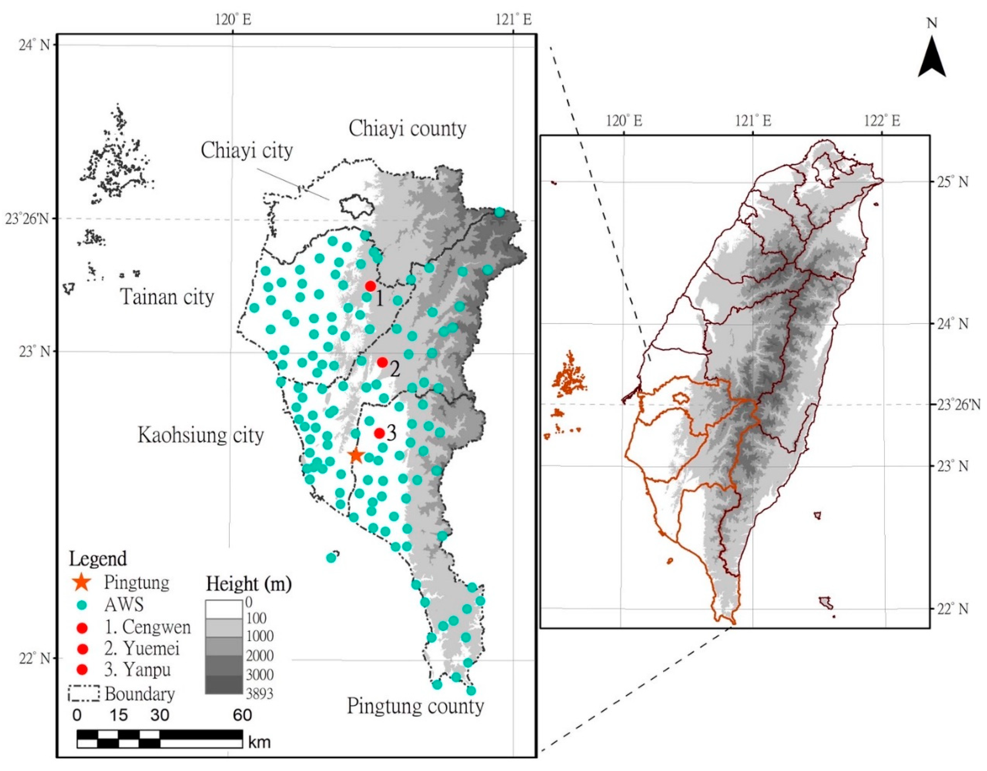
2.1. Study Area and Period

Southern Taiwan covers the areas of Chiayi, Tainan, Kaohsiung, and Pingtung from north to south (Figure 1). The study area was located near Pingtung Airport (22.7° N, 120.5° E, Figure 1), which has a higher percentage of rainfall associated with ATs than airports in eastern [35] and northern Taiwan [36]. Another reason for choosing this airport was that it is one of the four airports in Taiwan equipped with a Doppler lidar wind profiler. Pingtung Airport has a relatively flat terrain that serves as a good location to observe the effects of local circulations, such as the sea–land breeze and mountain–valley breeze, under weak synoptic weather conditions. An AT event on 5 August 2018, near Pingtung Airport was analyzed. The selected event day featured weak synoptic weather conditions that were mainly affected by local circulation. A detailed discussion of the event day is presented in Section 3.1.

2.2. Observational Data

A Doppler lidar wind profiler (LeoSphere Windcube 100S, Leosphere, France) with high spatial resolution (≤25 m) and temporal resolution (25 s) was used in the data assimilation system of the WRF model. The 134 AWSs in southern Taiwan (Figure 1) provided surface measurements of pressure, wind direction, wind speed, and precipitation. The wind information from 134 AWSs was adopted to understand the environment fields of the event day. The 12-h accumulated rainfall measurements from the 134 AWSs were analyzed and compared with model simulations with or without data assimilation of the lidar wind profiler at Pingtung Airport. Composite radar reflectivity maps were obtained from the Taiwan Central Weather Bureau (CWB; https://www.cwb.gov.tw/V8/C/W/OBS_Radar.html, accessed on 22 December 2021).

Before assimilation in the WRF model, the data of wind profiler with high vertical resolution were processed by two steps: (1) quality control and; (2) vertical thinning of profile data. Firstly, a quality control method of Ref. [37] was performed on wind profile data. Wind data were eliminated as the wind speed measurements associated with a Carrier-to-Noise Ratio’s outside the range of −25 to 5 dB. Secondly, observations of the wind profiler were thinning as the data closed to the model vertical levels. This step provided help in reducing the negative impacts due to vertical correlation occurring in high-density observations [27,28]. After the quality control and vertical thinning of wind profiler data at Pingtung Airport, the winds were separated into u (east-west direction) and v (north-south direction) components, and incorporated into model simulated data. Abnormal winds in Figure 2a were not found in Figure 2b, implying better data quality in the thinning profile than in the initial profile.

A manually operated surface meteorological station in Pingtung (Figure 1) is also located in Pingtung Airport. To assess the effect of ATs near Pingtung Airport on the event day, hourly visibility and precipitation from the Pingtung station and hourly surface pressure and precipitation from the Cengwen, Yuemei, and Yanpu stations (Figure 1) were used. The last three stations, located in southern Taiwan in the cities of Tainan, Kaohsiung, and Pingtung, respectively, were selected as they recorded the most extreme 6-h accumulated precipitation during the event day.

2.3. WRF Model Configuration and Experimental Design in Data Assimilation

In this study, the WRF model (version 3.8.1; Ref. [38]) and a data assimilation system based on WRF Variational Analysis (WRFVAR, version 3.9.1; Ref. [39]) were used for forecasting. The Doppler lidar wind profiler data were assimilated into the WRF-3DVAR system for prediction of the AT event on 5 August 2018.

The WRF model domain is centered on Taiwan, and has 451 × 451 horizontal grid points with horizontal resolutions of 2 km × 2 km, covering southeast China (19.5°–27.8° N, 116.4°–125.6° E). The domain has 52 vertical layers from the surface to a 20-hPa isobaric layer using a terrain following sigma coordinate. The physics schemes used in all domain include the Rapid Radiative Transfer Model longwave radiation and shortwave radiation [40], the Yonsei University planetary boundary layer scheme [41], the Unified Noah land surface scheme [42], and the Goddard microphysics scheme [43] instead of the cumulus scheme.

Radar data and surface observations including those from manually operated meteorological stations and AWSs provided the initial and boundary conditions of the WRF model, namely the Radar WRF operated by the Taiwan CWB (CWB RWRF). This WRF-3DVAR system assimilating both radar and surface observations is an assimilation forecasting system for convective scale and its lateral boundary forcing is updated every 1 h with a 13-h length.

The WRF–3DVAR system can be categorized as a data assimilation system that provides an analysis $x^a$ through minimizing the cost function J(x) [44] as follows.

$$\mathrm{J}\left(x\right)=\frac{1}{2}{\left(x_f^{\prime }\right)}^T{B}^{-1}\left(x_f^{\prime }\right)+\frac{1}{2}{\left(y-H\left[x\right]\right)}^T{R}^{-1}\left(y-H\left[x\right]\right)=J_b+J_o$$

(1)

$$x_f^{\prime }=x-x^b$$

(2)

where $\mathrm{J}\left(x\right)$ is the cost function of the atmospheric state. The background term $J_b$ plays a key role in the performance of data assimilation and it represents the analysis increment $x_f^{\prime }$. The observation term $J_o$ represents the distance between the vector of observation $y^o$ and the analysis observation vector transformed by the observation operator $H\left[x\right]$, which maps state space to observation space. The analysis increment $x_f^{\prime }$ is defined as the distance between the analysis state $x$ and the initial background field value $x^b$. The terms $B$ and $R$ are the covariance matrix of background and observation errors, respectively. In practice, R is often assumed to be static and diagonal, and is provided prior to the assimilation [45]. B is calculated using the approach of the National Meteorological Center [46] with option 3 (CV3; Ref. [47]) to build the background error covariance in 3DVAR.

To evaluate the impact of the data assimilation methods of the lidar wind profiler on AT prediction near Pingtung Airport, three groups—C1, C2 and C3—were used in our experimental design. In the C1 group, the experiments did not include data assimilation (

Table 1. Design of experiments.

Group	Experiments	Assimilation Time	Forecast Time
C1	NDA01	Without assimilation	0100–1300 UTC
	NDA02	Without assimilation Without assimilation	0200–1400 UTC
	NDA03		0300–1500 UTC
	NDA04	Without assimilation	0400–1600 UTC
C2	DA01	0100 UTC	0100–1300 UTC
	DA02	0200 UTC	0200–1400 UTC
	DA03	0300 UTC	0300–1500 UTC
	DA04	0400 UTC	0400–1600 UTC
C3	CDA01	0100–0400 UTC (hourly)	0400–1300 UTC
	CDA02	0200–0400 UTC (hourly)	0400–1400 UTC
	CDA03	0300–0400 UTC (hourly)	0400–1500 UTC

) and the initial and lateral boundary conditions with a horizontal resolution of 2 km were obtained from the Taiwan CWB RWRF. Subsequently, 12-h forecasts on a 2-km grid were launched at the starting times of 0100, 0200, 0300, and 0400 UTC on 5 August 2018, for the experiments NDA01, NDA02, NDA03, and NDA04, respectively (0100–1300, 0200–1400, 0300–1500, and 0400–1600 UTC, respectively; Table 1 and Figure 3).

In the C2 group, a single data assimilation strategy [48] suitable for the current operating procedure at the weather center was used. For the experiments DA01, DA02, DA03 and DA04, the outputs of the Taiwan CWB RWRF at 0100, 0200, 0300 and 0400 UTC were adopted, respectively, as the first guess (Figure 3). This step in the C2 group was the same as that in the C1 group; however, the following steps were different. The wind data at 63 different vertical levels above ground level (from 50 to 1600 m with an interval of 25 m) from the wind profiler at Pingtung Airport were assimilated into the 2-km-resolution domain, and the method of the National Meteorological Center [46] is adopted with option CV3 [47] to estimate background error covariance for assimilation of wind profiler observations. Finally, 12-h forecasts on a 2-km grid were launched at the starting times of 0100, 0200, 0300, and 0400 UTC on 5 August 2018, for the experiments DA01, DA02, DA03, and DA04, respectively (Table 1 and Figure 3).

In the C3 group, the data of Doppler lidar wind profiler were assimilated hourly starting from 0100 UTC, 0200 UTC, and 0300 UTC, respectively, and all of them ended at 0400 UTC. Finally, the 9-h, 10-h, and 11-h forecasts on a 2-km grid were launched at 0400 UTC, respectively, for experiments of CDA01, CDA02, and CDA03 (Table 1 and Figure 3).

2.4. Verification Methods

The forecasts of precipitation at the surface were verified against the observations of the 134 AWSs in southern Taiwan (Figure 1) over the model domain. Forecast performance of precipitation was evaluated using root-mean-square error (RMSE), Pearson product–moment correlation coefficient (PPMCC; Ref. [49]), and Spearman rank correlation coefficient (SRCC; Ref. [50]). Verification scores used were the threat score (TS; Ref. [51]) and bias score (BS; Ref. [49]). The calculation methods for the aforementioned coefficients and scores are defined as follows.

$$\mathrm{RMSE}=\sqrt{\frac{{{\displaystyle \sum }}_{\mathrm{i}=1}^{\mathrm{n}}{{(\mathrm{P}}_{\mathrm{i}}-{\mathrm{O}}_{\mathrm{i}})}^2}{\mathrm{n}}}$$

(3)

$$\mathrm{PPMCC}=\frac{{\sum }_{\mathrm{i}=1}^{\mathrm{n}}\left({\mathrm{P}}_{\mathrm{i}}-\overline{\mathrm{P}}\right)\left({\mathrm{O}}_{\mathrm{i}}-\overline{\mathrm{O}}\right)}{\sqrt{{\sum }_{\mathrm{i}=1}^{\mathrm{n}}{\left({\mathrm{P}}_{\mathrm{i}}-\overline{\mathrm{P}}\right)}^2}\sqrt{{\sum }_{\mathrm{i}=1}^{\mathrm{n}}{\left({\mathrm{O}}_{\mathrm{i}}-\overline{\mathrm{O}}\right)}^2}}$$

(4)

where ${\mathrm{P}}_{\mathrm{i}}$, ${\mathrm{O}}_{\mathrm{i}}$ and n refer to the predicted value, observed value and the number of observations, respectively. $\overline{\mathrm{P}}$, and $\overline{\mathrm{O}}$, refer to the sample mean for predicted value, and the sample mean for observed value, respectively.

$$\mathrm{SRCC}=1-\frac{6{{\displaystyle \sum }}_{\mathrm{i}=1}^{\mathrm{n}}{\mathrm{d}}_{\mathrm{i}}^2}{{\mathrm{n}(\mathrm{n}}^2-1)}$$

(5)

where ${\mathrm{d}}_{\mathrm{i}}$ refers to the difference between the two ranks of prediction and observation.

$$\mathrm{TS}=\raisebox{1ex}{$\mathrm{C}$}\!\left/ \!\raisebox{-1ex}{$(\mathrm{F}+\mathrm{O}-\mathrm{C})$}\right.$$

(6)

$$\mathrm{BS}=\raisebox{1ex}{$\mathrm{F}$}\!\left/ \!\raisebox{-1ex}{$\mathrm{O}$}\right.$$

(7)

where F, O, and C refer to the numbers of forecast points, observed points, and correctly forecast points with precipitation occurrence (hits; binary value is one), respectively.

The TS ranges from zero (no skill) to one (perfect skill). The BS ranges from positive infinity (over-forecasting) to negative infinity(under-forecasting), with a score of one representing the best performance of the model. The RMSE ranges from zero to positive infinity. The smaller the RMSE is, the better the model performance is. The PPMCC ranges from −1 to 1, with 1 representing the best performance of the model. The SRCC ranges from −1 to 1, with 1 representing the perfect monotonic relationship (a direct association) between observed and simulated data.

To verify forecast performance in comparison with the observations of 134 the AWSs, the 6-h accumulated precipitations from 0500 UTC to 1100 UTC (the black box of Figure 2), the major impact period of the AT event, were adopted from the 12-h precipitation operational forecasts of the WRF model. The quantitative precipitation forecast (QPF) skills such as TS and BS under data assimilation simulations for 6-h accumulated precipitation with thresholds of 5, 15, 10, and 20 mm were also calculated. Similar to the calculations of the RMSE, PPMCC, and SRCC, the TS and BS calculations were first performed by interpolation from the model grid data to station locations.

3. Results

3.1. Overview of the Event Day

When synoptic forcing is weak, most of the convection is triggered by diurnal heating during summer months in Taiwan [52]. On 5 August 2018, a weak synoptic-scale forcing environment was dominant in southern Taiwan. As ATs on the event day had a major impact during 0500–1100 UTC with a maximum precipitation intensity during 0600–0800 UTC, the following discussion mainly focused on the period of 0600–0800 UTC.

After sunrise, a sea breeze began to form in the coastal areas of southern Taiwan due to the increasing difference between the air temperature over land and over sea. As indicated by surface wind observations at 0600 UTC (1400 LST; Figure 4a), the sea breeze formation in southern Taiwan increased the surface wind speed as the prevailing winds and the sea breeze were from the northwest, and the observed peak wind speed in the southern coastal regions of Taiwan was 8–12 kt. However, the wind speed decreased as the wind moved inland. The convective activity around the mountains in southern Taiwan was enhanced after the air from the sea breeze was forced to move upward along the mountains. High composite radar reflectivity greater than 45 dBZ (Figure 4d) signifying intense precipitation that was closely associated with thunderstorms, was largely observed in the mountain regions of Chiayi, Kaohsiung and Pingtung. Due to the effect of convection cells with high composite radar reflectivity of 45 dBZ, intense precipitation occurred, which reduced the horizontal visibility of the Pingtung meteorological station located at Pingtung Airport (Figure 1) from 10 km to 8 km (Figure 5a).

Surface wind observations at 0700 UTC (1500 LST) revealed that the convective activity increased sharply on the land surface (Figure 4b), and the convection cells with high composite radar reflectivity (>45 dBZ) moved west toward the coast of southern Taiwan. As the onshore wind was strengthened due to the sea breeze effect, the convergence zone occurred at a smaller scale. Convergence lines (Figure 4e) formed rows of showers or thunderstorms, including over Chiayi, Tainan, Kaohsiung and Pingtung, and maximum surface wind speeds (Figure 4b) were approximately 18–22 kt over the area in the northeast of Pingtung Airport. Even though no obvious rainfall variations occurred in Pingtung Airport, horizontal visibility at the Pingtung weather station (star sign in Figure 1) gradually decreased from 8 km to 7 km (Figure 5a).

Surface wind observations at 0800 UTC (1600 LST) revealed the convergence line (Figure 4c) along the coast area. The composite radar reflectivity (Figure 4f) of Pingtung indicated that the row of thunderstorm had passed over Pingtung Airport. Under the influence of thunderstorm, horizontal visibility at the Pingtung meteorological station decreased from 7 to 5 km (Figure 5a). To reduce the risk of aviation accidents, pilots in Pingtung Airport are prohibited from flying under visual flight rules and are required to obey the instrument flight rules when horizontal visibility is less than or equal to 5 km. Therefore, although the observed maximum hourly rainfall was only approximately 2.5 mm (Figure 5a) during 0700–0800 UTC, the reduced horizontal visibility of 5 km exerted a great impact on aviation operations.

As the thunderstorm moved offshore and began to weaken, the horizontal visibility at the Pingtung meteorological station during 0900–1200 UTC (1700–2000 LST) increased from 6 to 9 km (Figure 5a). Under the impact of the thunderstorm from 0600 to 1200 UTC, storm cells resulted in short-duration intense rainfall in many areas and caused a decrease in atmospheric visibility. The 6-hr accumulated precipitation during 0600–1200 UTC at Cengwen (Figure 5b), Yuemei (Figure 5c), and Yanpu (Figure 5d) was 55, 77.5, and 43 mm, respectively, and the 1-hr maximum precipitation occurred at 1600 UTC for the three stations. The precipitation measured at the Cengwen, Yuemei, and Yanpu station fit the requirements of a short-duration intense rainfall event as the rainfall exceeded 30 mm during a 12-h period (Yang et al., 2017). The Pingtung meteorological station recorded precipitation of less than 30 mm in six hours. However, the horizontal visibility of Pingtung Airport less than 5 km reached the condition of prohibiting pilots to fly. The reduced horizontal visibility at Pingtung Airport might have been due to strong rainfall around the area (Figure 4f). As the thunderstorm approached, the surface pressure continued to drop greatly for the Cengwen (Figure 5b), Yuemei (Figure 5c), and Yanpu (Figure 5d) stations until the front passed completely. The lowest surface pressures measured by the three stations were 989.2, 990.7, and 998.6 hPa at the Cengwen (Figure 5b), Yuemei (Figure 5c), and Yanpu (Figure 5d) stations, respectively, during the afternoon from 0500 to 0700 UTC.

The observed, DA01 assimilated, NDA01 non-assimilated hourly surface pressure, temperature and dew-point temperature of Pingtung Airport from 0100 to 0900 UTC (0900 to 1700 LST) on 5 August 2018 are shown in Figure 6. The changes of surface pressure (Figure 6a), temperature (Figure 6b) and dew-point temperature (Figure 6c) were quite similar in observations, simulations with data assimilation and without data assimilation. Although the rainfall time was 1600 LST at Pingtung (Figure 5a), surface pressure (Figure 6a) and temperature (Figure 6b) dropped rapidly from 0400 to 0600 UTC (1200 LST to 1400 LST), due to the sea breeze effect associated with cool moist air. Then the dew-point temperature (Figure 6c) increased to promote cloud development and block solar radiation.

Compared with DA01 assimilated simulations, the changes of surface pressure (Figure 6a) and temperature (Figure 6b) of NDA01 non-assimilated simulations during 0100–0700UTC were closer to those of observations, which were caused by stronger sea breeze in DA01 than in NDA01 simulations and will be examined in Figures 8–10. However, further examination of the time period during 0500–1000 UTC in DA01 and NDA01 simulations revealed that the surface pressure (Figure 7a) and temperature (Figure 7c) of DA01 assimilated simulations after 0700 UTC were closer to those of observations than those of NDA01 non-assimilated simulations, which were caused by the effect of more accurate precipitation in DA01 than in NDA01 simulations. More accurate rainfall forecast in the model simulations tends to have variables such as atmospheric pressure and temperature closer to observations. The DA02 simulations performed better in rainfall forecast than the DA01 and DA03 simulations, and will be further examined in the following sections. Compared with the DA01 (Figure 7a,c) and NDA02 (Figure 7b,d) simulations, the changes of surface pressure (Figure 7b) and temperature (Figure 7d) in the DA02 simulations had a closer distribution to those of observations.

In summary, on 5 August 2018, the sea breeze gradually increased in southern Taiwan in the afternoon as the sun continued to warm the land. Convective motions with high radar reflectivity were driven. At 0700 UTC, a row of thunderstorms formed over Chiayi, Tainan, Kaohsiung and Pingtung and reached the mature stage (Figure 4e). Wind speeds (Figure 4b) near the surface increased along the east and west sides of the thunderstorm, and a clear convergence zone was established (Figure 4b), which was geographically located in the regions of 120.4° E–120.9° E and 22.4° N–22.6° N (Figure 4e). At 0800 UTC, as sea breezes gradually changed into land breezes along the coastal regions (Figure 4c–f), the thunderstorm moved west and became weaker, and the northwesterly wind changed to a weak southeasterly wind at many stations. Aviation operations had a great change from visual flight rules to instrument flight rules at Pingtung Airport in the afternoon, as the observed horizontal visibility reduced from 8 to 5 km in 2 h (0600–0800 UTC) under the influence of the ATs.

3.2. Verification of the ATs

In this section, the 6-h accumulated precipitation from forecasts launched between 0500 and 1100 UTC, the major impact period of ATs, was verified. We first compared groups C1, C2 and C3 in predicting the location, intensity, and wind field of the ATs. Subsequently, verification methods were used to evaluate the forecast performance of each group.

Compared with the observations (Figure 8l), the simulated accumulated precipitation of group C1 without data assimilation (NDA01–04) revealed incorrect positions and underestimated precipitations of the ATs (Figure 8a–d). In contrast to group C1, there was significant improvement with respect to the distribution of precipitations of ATs in the 3DVAR experiments of data assimilation for groups C2 (Figure 8e–h) and C3 (Figure 8i–k). In group C3, CDA01 (Figure 8i), CDA02 (Figure 8j) and CDA03 (Figure 8k) experiments used the same initial time as that of DA04 (Figure 8h). However, CDA02, assimilated during 0200-0400 UTC, and CDA03, assimilated during 0300-0400 UTC, had stronger intensity of precipitation than that of DA04. The overall forecasting abilities of precipitations between observations and CDA02, CDA03 and DA04 simulations were pretty close. The quantitative comparison between them will be further examined in Section 3.3. The precipitation in CDA01 assimilated during 0100-0400 UTC periods was underestimated on the west coast close to Tainan due to significant northeasterly at 0100 UTC, causing downdraft and a stable atmosphere in the leeward side of the mountains.

The observed and simulated 10-m wind field and lowest model-level radar reflectivity for the C1 and C2 AT forecasts are illustrated in Figure 9 and Figure 10, respectively. Panels in the top row in both figures represent the observed ATs, and panels in the other rows illustrate the forecasted ATs. Compared with the observed data (Figure 9a–c), the C1 simulations without data assimilation revealed incorrect tracks of the AT movement toward the west coast of southern Taiwan during 0600 UTC, 0700 UTC, and 0800 UTC, and the simulated onshore wind was clearly underestimated for the experiments of NDA01 (Figure 9d–f), NDA02 (Figure 9g–i), NDA03 (Figure 9j–l), and NDA04 (Figure 9m–o). A substantial improvement with respect to the distribution of wind fields and the intensity and locations of ATs was evident in the C2 simulations with data assimilation in the 3DVAR experiments of DA01, DA02, DA03, and DA04.

At 0600–0800 UTC in the C2 group, the AT entered its mature stage. From 0600 to 0700 UTC, the onshore wind was strengthened by the sea breeze effect on the coasts of Tainan, Kaohsiung, and Pingtung in the experiments of DA01 (Figure 10d,e), DA02 (Figure 10g,h), DA03 (Figure 10j,k), and DA04 (Figure 10m,n), and the maximum surface wind speed ranged from 8 to 12 kt. From 0700 to 0800 UTC, as the AT developed and moved to the west, the wind on the east side of the ATs shifted to east-southeast in the experiments of DA01 (Figure 10e,f), DA02 (Figure 10h,i), DA03 (Figure 10k,l), and DA04 (Figure 10n,o).

A vertical cross-section of the precipitation radar echoes in the C1 experiments without data assimilation, NDA02 (Figure 10a–c) as an example, the locations of AT development were farther west, the ATs moved much faster, and precipitation radar echoes of ATs dissipated quicker than those of observations. A vertical cross-section of the precipitation radar echoes in the C2 experiments (Figure 11) revealed that the onshore wind from the west coast and downdrafts collided on the surface, triggering deep convection with high radar reflectivity as in Ref. [52], especially for the experiments of DA02, DA03, and DA04. The ATs associated with deep convection with sufficient convergence extended from near the surface to above 10 km vertically (Figure 11). In contrast to the C1 experiments, the C2 experiments DA02, DA03, and DA04 revealed substantial improvements and successfully forecasted the mature stage of ATs at 0700 UTC, which was characterized by vigorous updrafts and downdrafts [53,54,55]. Compared with the observations, DA02 exhibited more accurate results in forecasting the locations and intensities of ATs and the associated wind fields than did the other three experiments of DA01, DA03, and DA04.

To have a common basis for comparison of vertical cross sections of the precipitation radar echoes between the C2 and C3 experiments, it is better to use the same initial forecast time of model simulations. Therefore, DA04 (Figure 12j–l) of C2 experiments and CDA03 (Figure 13a–c) of C3 experiments, which both had the same initial forecast time and better forecast performance, were used as examples for comparisons. In contrast to the C2 DA04 experiment, the C3 CDA03 experiment was similar in the locations of convective cells but quite different in the convective intensity. At 0700 UTC (Figure 13b), the convective intensity of the C3 CDA03 experiment at the east of Pingtung Airport was weaker than that of the C2 DA04 experiment (Figure 12k). However, two convective cells formed at the west of Pingtung Airport in the C3 CDA03 experiment were stronger than those at the same location in the C2 DA04 experiment.

The quantitative analysis of the overall rainfall of the model simulations with data assimilation under the C2–C3 experiments in southern Taiwan examined in the next section will demonstrate that the performances of CDA02 and CDA03 in the C3 experiments were better than those of DA02 and DA03 in the C2 experiments.

3.3. Quantitative Analysis for Precipitation Forecast

An evaluation of the model QPF was conducted using the scores of TS, BS, RMSE, PPMCC and SRCC, as defined in Section 2.4. The surface forecasts of the C1, C2 and C3 experiments were compared with the AWS observations. At the thresholds of 5, 10, 15, and 20 mm, the differences between the forecasts and observations for the 6-h accumulated precipitation were compared to examine forecast performance.

Compared with group C1, groups C2 and C3 revealed substantial improvement in TS, with higher scores closer to one for the different thresholds of 6-h accumulated precipitation (Figure 14a). Among the C2 experiments, DA02 had the highest TS at the threshold of 5 mm but a lower TS at the thresholds of 10, 15, and 20 mm. DA03 had the highest TS at the threshold of 5 mm but a lower TS at the thresholds of 10, 15, and 20 mm. DA04 had a TS higher than or comparable to that of the other experiments for the thresholds of 5, 10, and 15 mm but a lower TS at thresholds of 20 mm. Among the C3 experiments for most of the thresholds, CDA01 had the lowest TS, and CDA02 and CDA03 had highest TS.

Forecasting performance under different experiments was better if the BS was closer to one (Figure 14b). All C1 experiments with a BS < 1 provided an underestimated forecast for the different thresholds. C2 experiment DA04 and C3 experiment CDA04 also had a BS < 1 and featured an underestimated forecast. However, C2 experiments of DA01, DA02 and DA03 and C3 experiments of CDA02 and CDA03 generally had BS > 1 and produced an overestimated forecast. Similar to the TS (Figure 14a), at the thresholds of 15 and 20mm, the BS had better scores close to one in the group C2 than in the group C1 (Figure 14b). Among the C2 experiments, DA04 had the highest skill of the BS at all thresholds, followed by DA02 and DA01 (Figure 14b). Among the C1 experiments, NDA03 and NDA04 had better skill of the BS at the thresholds of 5 and 10 mm (Figure 14b).

For the C1 and C2 group experiments, TS and BS tended to be higher at the thresholds of 5 and 10 mm than at 15 and 20 mm. Higher thresholds with lower scores might be due to the low forecast quality or lower number of observation stations for verification for the 6-h accumulated precipitation. For the thresholds of 5, 10, 15, and 20 mm, the station numbers (percentage of station numbers for different thresholds relative to the total station numbers) were 70 (52%), 18 (13%), 12 (9%), and 8 (6%), respectively.

A smaller RMSE indicates superior forecasting performance in the experiments. PPMCC and SRCC values closer to one also indicate better forecasting performance. The RMSE values (Figure 15a) revealed that the C2 experiment DA04 and C3 experiment CDA01 performed better than other experiments due to lower RMSE. In contrast, C2 experiments DA01 and DA03, and C3 experiment CDA02 had higher RMSE.

The PPMCC values (Figure 15a) revealed that C2 performed better than C1 in all four experiments, with significant improvement in DA03 and DA04. Among all the experiments, CDA03 was the best-performing one. Among C2 experiments, DA04 was the best-performing, with an RMSE of 16.3 mm and a correlation coefficient of 0.3.

The spatial variability of the SRCC between the forecasted and observed 6-h accumulated precipitation (Figure 15b) revealed that a positive correlation between forecasted and observed 6-h accumulated precipitation across the study area was found in all C1, C2 and C3 experiments. Compared with the group C1, the C2 group exhibited a much higher correlation between forecasts and observations in the experiments of DA02, DA03, and DA04, but not DA01. The higher correlation (SRCC values closer to 0.5) with statistical significance (p < 0.05) was observed in DA02, DA04, CDA02 and CDA03. Overall, RMSE, PPMCC, and SRCC analyses demonstrated that the simulations with data assimilation under C2 and C3 experiments performed better than those without data assimilation under C1 experiments. C2 experiment DA04 and C3 experiments performed best among all the experiments, implying that the performance of precipitation prediction gradually increased as the implementation time of data assimilation became closer to the target period of 0500 to 1100 UTC, that is, the occurrence of ATs.

4. Discussion and Conclusions

The main goal of this study was to evaluate the performance of experiments with and without data assimilation for predicting the ATs near Pingtung Airport on 5 August 2018. In the experiments with data assimilation, the 3DVAR system of the WRF model was assimilated with observation data from the Doppler lidar wind profiler in Pingtung Airport.

During the major impact period of 0500–1100 UTC (1300–1900 LST) on 5 August 2018, ATs triggered by sea breeze circulation gradually formed in southern Taiwan and reached their mature stage at 0700 UTC, resulting in a single, quasi-stationary line of convection along the west coast. Short-duration intense rainfall of more than 30 mm during 12 h was observed in data collected from the AWSs of the Cengwen, Yuemei, and Yanpu stations. This reduced horizontal visibility to ≤5 km at the Pingtung meteorological station, which limited pilots to fly only under the instrument flight rules instead of visual flight rules. The change of flight rules exerted a great impact on aviation operations.

Compared with the C1 experiments without data assimilation (NDA01, NDA02, NDA03 and NDA04), the C2 experiments (DA01, DA02, DA03 and DA04) and the C3 group experiments (CDA01, CDA02, CDA03) that used the 3DVAR system with wind profiler data exhibited greatly improved simulation accuracy of the locations, intensity of ATs and wind fields produced by the local circulations of the sea breeze and the mountains in southern Taiwan in the horizontal and vertical directions.

The model QPF was also greatly improved in the experiments with data assimilation. The TS of the C2 experiments exhibited consistently higher skills at the thresholds of 5, 10, 15 and 20 mm than did those of the C1 experiments. Similarly, the BS of the C2 experiments had mostly higher skills at the various thresholds. For all the C1 and C2 experiments, TS and BS tended to be higher at the thresholds of 5 and 10 mm than those of 15 and 20 mm. The analyses of PPMCC and SRCC also revealed the better model performance in the C2 and C3 group experiments with data assimilation. Among the group C2, the DA04 experiment performed best in the analysis of BS, TS, RMSE, PPMCC and SRCC and performed comparable to the DA02 experiment in the analysis of BS. Thus, the DA04 experiment had the overall better evaluation than other experiments of DA01, DA02 and DA03. However, the TS was higher in CDA02 and CDA03 in DA04, which implies that as the implementation time of data assimilation approaches the occurrence time of ATs, the forecast performance of short-duration intense rainfall is greatly improved.

As in the study of Ref. [56], our findings suggest that assimilation of Doppler lidar wind profiles into a WRF-3DVAR system creates conditions that favor the development of ATs and upscale growth. Although the results of this study are only supported by a single case, they provide valuable clues to improve the prediction of ATs by using the assimilation of lidar wind profiler data at Pingtung Airport. In the future, more case studies of the assimilation of lidar wind profiler data should be conducted to improve the accuracy and applicability of the results.

References

1. Yang, P.; Ren, G.; Yan, P. Evidence for a strong association of short-duration intense rainfall with urbanization in the Beijing urban area. J. Clim. 2017, 30, 5851–5870. [Google Scholar] [CrossRef]
2. Fowler, H.J.; Lenderink, G.; Prein, A.F.; Westra, S.; Allan, R.P.; Ban, N.; Barbero, R.; Berg, P.; Blenkinsop, S.; Do, H.X.; et al. Anthropogenic intensification of short-duration rainfall extremes. Nat. Rev. Earth Environ. 2021, 2, 107–122. [Google Scholar] [CrossRef]
3. Bouttier, F.; Marchal, H. Probabilistic thunderstorm forecasting by blending multiple ensembles. Tellus A Dyn. Meteorol. Oceanogr. 2020, 72, 1–19. [Google Scholar] [CrossRef] [Green Version]
4. Wu, C.-M.; Lin, H.-C.; Cheng, F.-Y.; Chien, M.-H. Implementation of the Land Surface Processes into a Vector Vorticity Equation Model (VVM) to Study its Impact on Afternoon Thunderstorms over Complex Topography in Taiwan. Asia-Pac. J. Atmos. Sci. 2019, 55, 701–717. [Google Scholar] [CrossRef]
5. Kerns, B.W.J.; Chen, Y.L.; Chang, M.Y. The diurnal cycle of winds, rain, and clouds over Taiwan during the mei-yu, summer, and autumn rainfall regimes. Mon. Weather Rev. 2010, 138, 497–516. [Google Scholar] [CrossRef]
6. Ruppert, J.H.; Johnson, R.H.; Rowe, A.K. Diurnal circulations and rainfall in Taiwan during SoWMEX/TiMREX (2008). Mon. Weather Rev. 2013, 141, 3851–3872. [Google Scholar] [CrossRef] [Green Version]
7. Huang, W.-R.; Chen, K.-C. Trends in pre-summer frontal and diurnal rainfall activities during 1982–2012 over Taiwan and Southeast China: Characteristics and possible causes. Int. J. Climatol. 2015, 35, 2608–2619. [Google Scholar] [CrossRef]
8. Chen, T.-C.; Yen, M.-C.; Tsay, J.-D.; Liao, C.-C.; Takle, E.S. Impact of afternoon thunderstorms on the land-sea breeze in the Taipei basin during summer: An experiment. J. Appl. Meteor. Climatol. 2014, 53, 1714–1738. [Google Scholar] [CrossRef]
9. Chen, T.-C.; Tsay, J.-D.; Takle, E.S. Interannual Variation of Summer Rainfall in the Taipei Basin. J. Appl. Meteorol. Climatol. 2016, 55, 1789–1812. [Google Scholar] [CrossRef]
10. Miao, J.-E.; Yang, M.-J. A modeling study of the severe afternoon thunderstorm event at Taipei on 14 June 2015: The roles of sea breeze, microphysics, and terrain. J. Meteor. Soc. Jpn. 2020, 98, 129–152. [Google Scholar] [CrossRef] [Green Version]
11. Chen, T.C.; Wang, S.Y.; Yen, M.C. Enhancement of afternoon thunderstorm activity by urbanization in a valley: Taipei. J. Appl. Meteor. Climatol. 2007, 46, 1324–1340. [Google Scholar] [CrossRef]
12. Chen, T.-C.; Tsay, J.-D.; Takle, E.S. A Forecast Advisory for Afternoon Thunderstorm Occurrence in the Taipei Basin during Summer Developed from Diagnostic Analysis. Weather Forecast. 2016, 31, 531–552. [Google Scholar] [CrossRef]
13. Cao, Y.; Wu, Z.; Xu, Z. Effects of rainfall on aircraft aerodynamics. Prog. Aerosp. Sci. 2014, 71, 85–127. [Google Scholar] [CrossRef]
14. Tsujino, S.; Kuo, H.-C.; Yu, H.; Chen, B.-F.; Tsuboki, K. Effects of mid-level moisture and environmental flow on the development of afternoon thunderstorms in Taipei. Terr. Atmos. Ocean. Sci. 2021, 32, 497–518. [Google Scholar] [CrossRef]
15. Johnson, R.H.; Breach, J.F. Diagnosed characteristics of precipitation systems over Taiwan during the May–June 1987 TAMEX. Mon. Weather Rev. 1991, 119, 2540–2557. [Google Scholar] [CrossRef]
16. Chen, Y.-L.; Li, J. Characteristics of surface airflow and pressure patterns over the island of Taiwan during TAMEX. Mon. Weather Rev. 1995, 123, 695–716. [Google Scholar] [CrossRef] [Green Version]
17. Harding, K. Thunderstorm formation and aviation hazards. In The Front-NWS Aviation Weather Safety Updates; NOAA National Weather Service: Silver Spring, MD, USA, 2011; pp. 1–4. [Google Scholar]
18. Oo, K.T.; Oo, K.L. Analysis of the Most Common Aviation Weather Hazard and Its Key Mechanisms over the Yangon Flight Information Region. Adv. Meteorol. 2022, 5356563. [Google Scholar] [CrossRef]
19. Mazzarella, V.; Ferretti, R.; Picciotti, E.; Marzano, F.S. Investigating 3D and 4D variational rapid-update-cycling assimilation of weather radar reflectivity for a heavy rain event in central Italy. Nat. Hazards Earth Syst. Sci. 2021, 21, 2849–2865. [Google Scholar] [CrossRef]
20. Sun, J.; Wang, H.; Tong, W.; Zhang, Y.; Lin, C.-Y.; Xu, D. Comparison of the impacts of momentum control variables on high-resolution variational data assimilation and precipitation forecasting. Mon. Weather Rev. 2016, 144, 149–169. [Google Scholar] [CrossRef]
21. Wang, H.; Sun, J.; Fan, S.; Huang, X.-Y. Indirect assimilation of radar reflectivity with WRF 3D-Var and its impact on prediction of four summertime convective events. J. Appl. Meteorol. Clim. 2013, 52, 889–902. [Google Scholar] [CrossRef]
22. Floors, R.; Vincent, C.L.; Gryning, S.E.; Peña, A.; Batchvarova, E. The wind profile in the coastal boundary layer: Wind lidar measurements and numerical modelling. Bound.-Layer Meteorol. 2013, 147, 469–491. [Google Scholar] [CrossRef]
23. Ortiz-Amezcua, P.; Martínez-Herrera, A.; Manninen, A.J.; Pentikäinen, P.P.; O’Connor, E.J.; Guerrero-Rascado, J.L.; AladosArboledas, L. Wind and Turbulence Statistics in the Urban Boundary Layer over a Mountain–Valley System in Granada, Spain. Remote Sens. 2022, 14, 2321. [Google Scholar] [CrossRef]
24. Smith, T.L.; Benjamin, S.G. Impact of network wind profiler data on a 3-h Data Assimilation System. Bull. Am. Meteorol. Soc. 1993, 74, 801–807. [Google Scholar] [CrossRef] [Green Version]
25. Zhang, Y.; Chen, M.; Zhong, J.A. Quality Control Method for Wind Profiler Observations toward Assimilation applications. J. Atmos. Ocean. Technol. 2017, 34, 1591–1606. [Google Scholar] [CrossRef]
26. Wang, C.; Chen, Y.; Chen, M.; Shen, J. Data assimilation of a dense wind profiler network and its impact on convective forecasting. Atmos. Res. 2020, 238, 104880. [Google Scholar] [CrossRef]
27. Wang, C.; Chen, M.; Chen, Y. Impact of Combined Assimilation of Wind Profiler and Doppler Radar Data on a Convective-Scale Cycling Forecasting System. Mon. Weather Rev. 2022, 150, 431–450. [Google Scholar] [CrossRef]
28. St-James, J.S.; Laroche, S. Assimilation of wind profiler data in the Canadian Meteorological Center’s analysis system. J. Atmos. Ocean. Technol. 2005, 22, 1181–1194. [Google Scholar] [CrossRef]
29. Wang, C.-K. Impact of Assimilating the WINDAS Data for Precipitation in Eastern Taiwan-Typhoon MEGI. Master’s Thesis, Institute of Atmospheric Physics, National Central University, Taoyuan, Taiwan, 2013. (In Chinese with English abstract). [Google Scholar]
30. Zhang, X.B.; Luo, Y.L.; Wan, Q.L.; Ding, W.Y.; Sun, J.X. Impact of assimilating wind profiling radar observations on convection-permitting quantitative precipitation forecasts during SCMREX. Weather Forecast. 2016, 31, 1271–1292. [Google Scholar] [CrossRef]
31. Gregow, E. New Methods Using In-Situ and Remote-Sensing Observations for Improved Meteorological Analysis; Finnish Meteorological Institute: Helsinki, Finland, 2018; pp. 80–91. [Google Scholar]
32. Grund, C.J.; Banta, R.M.; George, J.L.; Howell, J.N.; Post, M.J.; Richter, R.A.; Weickmann, A.M. High-resolution Doppler lidar for boundary layer and cloud research. J. Atmos. Ocean. Technol. 2001, 18, 376–393. [Google Scholar]
33. Finn, T.S.; Geppert, G.; Ament, F. Towards assimilation of wind profile observations in the atmospheric boundary layer with a sub-kilometre-scale ensemble data assimilation system. Tellus A Dyn. Meteorol. Oceanogr. 2020, 72, 1–14. [Google Scholar]
34. Liu, D.; Huang, C.; Feng, J. Influence of Assimilating Wind Profiling Radar Observations in Distinct Dynamic Instability Regions on the Analysis and Forecast of an Extreme Rainstorm Event in Southern China. Remote Sens. 2022, 14, 3478. [Google Scholar] [CrossRef]
35. Yeh, N.-C.; Chuang, Y.-C.; Peng, H.-S.; Chen, C.-Y. Application of AIRS soundings to afternoon convection forecasting and nowcasting at Airports. Atmosphere 2021, 13, 61. [Google Scholar] [CrossRef]
36. Lin, P.-F.; Chang, P.-L.; Jou, B.J.-D.; Wilson, J.W.; Roberts, R.D. Warm Season Afternoon Thunderstorm Characteristics under Weak Synoptic-Scale Forcing over Taiwan Island. Weather Forecast. 2011, 26, 44–60. [Google Scholar] [CrossRef] [Green Version]
37. Bakhoday-Paskyabi, M.; Flügge, M. Predictive Capability of WRF Cycling 3DVAR: LiDAR Assimilation at FINO1. J. Phys. Conf. Ser. 2021, 2018, 012006. [Google Scholar]
38. Michalakes, J.; Dudhia, J.; Gill, D.; Henderson, T.; Klemp, J.; Skamarock, W.; Wang, W. The Weather Research and Forecast Model: Software architecture and performance. In Proceedings of the 11th Workshop on the Use of High Performance Computing in Meteorology, Reading, UK, 25–29 October 2004; ECMWF: Reading, UK, 2004; pp. 156–168. [Google Scholar]
39. Benjamin, S.G.; Grell, G.A.; Brown, J.M.; Smirnova, T.G.; Bleck, R. Mesoscale weather prediction with the RUC hybrid isentropic–terrain-following coordinate model. Mon. Weather Rev. 2004, 132, 473–494. [Google Scholar]
40. Mlawer, E.J.; Taubman, S.J.; Brown, P.D.; Iacono, M.J.; Clough, S.A. Radiative transfer for inhomogeneous atmospheres: RRTM, a validated correlated-k model for the longwave. J. Geophys. Res. 1997, 102, 16663–16682. [Google Scholar] [CrossRef] [Green Version]
41. Hong, S.; Noh, Y.; Dudhia, J. A new vertical diffusion package with an explicit treatment of entrainment processes. Mon. Weather Rev. 2006, 134, 2318–2341. [Google Scholar] [CrossRef] [Green Version]
42. Mukul Tewari, N.C.A.R.; Tewari, M.; Chen, F.; Wang, W.; Dudhia, J.; LeMone, M.; Mitchell, K.; Ek, M.; Gayno, G.; Wegiel, J.; et al. Implementation and verification of the Unified NOAH land surface model in the WRF model. In Proceedings of the 20th Conference on Weather Analysis and Forecasting/16th Conference on Numerical Weather Prediction, Seattle, WA, USA, 11–15 January 2004; pp. 11–15. [Google Scholar]
43. Tao, W.K.; Simpson, J.; McCumber, M. An ice–water saturation adjustment. Mon. Weather Rev. 1989, 117, 231–235. [Google Scholar] [CrossRef] [Green Version]
44. Ide, K.; Courtier, P.; Ghil, M.; Lorenc, A. Unified notationfor data assimilation: Operational, sequential and variational. J. Meteor. Soc. Jpn. 1997, 75, 181–197. [Google Scholar] [CrossRef] [Green Version]
45. Skamarock, W.C.; Klemp, J.B.; Dudhia, J.; Gill, D.O.; Baker, D.M.; Wang, W.; Powers, J.G. A Description of the Advanced Research WRF Version 2; NCAR Tech. Note NCAR/TN-468+STR; NCAR: Boulder, CO, USA, 2005; pp. 87–95. [Google Scholar]
46. Parrish, D.F.; Derber, J.C. The national meteorological center’s spectral statistical-interpolation analysis system. Mon. Weather Rev. 1992, 120, 1747–1763. [Google Scholar] [CrossRef]
47. Meng, Z.; Zhang, F. Test of an ensemble Kalman filter for mesoscale and regional-scale data assimilation. Part IV: Comparison with 3DVar in a month-long experiment. Mon. Weather Rev. 2008, 136, 3671–3682. [Google Scholar] [CrossRef]
48. Chen, I.-H.; Hong, J.-S.; Tsai, Y.-T.; Fong, C.-T. Improving afternoon thunderstorm prediction over Taiwan through 3DVar-based radar and surface data assimilation. Weather Forecast. 2020, 35, 2603–2620. [Google Scholar] [CrossRef]
49. Wang, Q.J.; Pagano, T.C.; Zhou, S.L.; Hapuarachchi, H.A.P.; Zhang, L.; Robertson, D.E. Monthly versus daily water balance models in simulating monthly runoff. J. Hydrol. 2011, 404, 166–175. [Google Scholar] [CrossRef]
50. Qian, C.; Zhou, W.; Fong, S.K.; Leong, K.C. Two approaches for statistical prediction of non-Gaussian climate extremes: A case study of Macao hot extremes during 1912–2012. J. Clim. 2015, 28, 623–636. [Google Scholar] [CrossRef]
51. Schaefer, J.T. The Critical Success Index as an Indicator of Warning Skill. Weather Forecast. 1990, 5, 570–575. [Google Scholar] [CrossRef] [Green Version]
52. Lin, P.-F.; Chang, P.-L.; Ben, J.-D. Warm season afternoon thunderstorm characteristics under weak synoptic-scale forcing over Taiwan island and its objective prediction. Atmos. Sci. 2012, 40, 77–108, (In Chinese with English abstract). [Google Scholar]
53. Houze, R.A., Jr. Cloud Dynamics, 2nd ed.; Elsevier/Academic Press: Oxford, UK, 2014; pp. 237–243. [Google Scholar]
54. Houze, R.A., Jr. 100 years of research on mesoscale convective systems. Meteor. Monogr. 2018, 59, 17.1–17.54. [Google Scholar] [CrossRef]
55. Wang, D.; Giangrande, S.E.; Feng, Z.; Hardin, J.C.; Prein, A.F. Updraft and downdraft core size and intensity as revealed by radar wind profilers: MCS observations and idealized model comparisons. J. Geophys. Res. Atmos. 2020, 125, e2019JD031774. [Google Scholar] [CrossRef]
56. Hristova-Veleva, S.; Zhang, S.; Turk, F.J.; Haddad, Z.S.; Sawaya, R. Assimilation of DAWN Doppler wind lidar data during the 2017 Convective Processes Experiment (CPEX): Impact on precipitation and flow structure. Atmos. Meas. Tech. 2021, 14, 3333–3350. [Google Scholar] [CrossRef]
Figure 1. The locations of 134 AWSs (green dots) used in this study. Variables of Pingtung meteorological station located at the Pingtung Airport (red star), and three AWSs of Cengwen (station 1, red dot), Yuemei (station 2, red dot), and Yanpu (station 3, red dot) were used to describe the background conditions of the event day.
Atmosphere 13 01341 g001
Figure 2. Comparisons between wind observations of (a) the initial profile and (b) thinning profile at Pingtung Airport from 0100 to 0400 UTC (0900 to 1200 LST) on 5 August 2018. Abnormal winds are represented by black circles in (a).
Atmosphere 13 01341 g002
Figure 3. Schematic diagram of data assimilation-forecast strategy for the 2-km mesh for experiments of C1(NDA01, NDA02, NDA03 and NDA04), C2(DA01, DA02, DA03 and DA04) and C3 (CDA01, CDA02 and CDA03). The black box represents the major impact period of the thunderstorm event.
Atmosphere 13 01341 g003
Figure 4. Surface wind observations (kt; vector) at (a) 0600, (b) 0700, and (c) 0800 UTC and composite radar reflectivity (dBZ; shaded) at (d) 0600, (e) 0700, and (f) 0800 UTC on 5 August 2018 from 134 AWSs. The location of Pingtung Airport (Pingtung meteorological station) was depicted as red star in (ac) and white star in (df), respectively. The blue lines in (ac) indicated the convergence line of ATs. Wind speeds more (less) than 8 kt were colored in red (black).
Atmosphere 13 01341 g004
Figure 5. Observed hourly visibility (km; blue line) and accumulated precipitation (mm; red bar) at (a) Pingtung meteorological station, and observed hourly surface pressure (hPa; blue line) and accumulated precipitation (mm; red bar) at the (b) Cengwen, (c) Yuemei and (d) Yanpu AWSs from 0400 to 1500 UTC (1200 to 2300 LST) on 5 August 2018.
Atmosphere 13 01341 g005
Figure 6. The observed (solid lines), DA01 assimilated (dot lines) and NDA01 non-assimilated (dashed lines) hourly surface (a) pressure, (b) temperature, (c) dew-point temperature of Pingtung Airport from 0100 to 0900 UTC (0900 to 1700 LST) on 5 August 2018.
Atmosphere 13 01341 g006
Figure 7. The hourly surface pressure for (a) observations (solid lines), DA01 (dot lines) and NDA01 (dashed lines) simulations, and for (b) observations (solid lines), DA02 (dot lines) and NDA02 (dashed lines) simulations of Pingtung Airport from 0500 to 1000 UTC (1300 to 1800 LST) on 5 August 2018. (c,d) are similar to (a,b), but for the hourly surface temperature. Note that Figure 7a,c are similar to Figure 6a,b, respectively, but different in the time span.
Atmosphere 13 01341 g007
Figure 8. The simulated accumulated precipitation (mm) during 0500-1100 UTC (1300-1900 LST) on 5 August 2018, (ad) NDA01-NDA04, (eh) DA01-DA04, (ik) CDA01-CDA03 simulations, and (l) observations.
Atmosphere 13 01341 g008
Figure 9. The observed and simulated 10-m wind (in arrow; intervals of 5 kt) and lowest model-level radar reflectivity (in color; dBZ) from 0600 to 0800 UTC (1400 to 1600 LST) on 5 August 2018, (ac) observations, same as Figure 4, (df) NDA01, (gi) NDA02, (jl) NDA03, and (mo) NDA04 simulations. Additionally shown are the approximate location of Pingtung Air Force Base (black star) and vertical cross-section planes (black line) for subsequent figures. The lines between x and x’ are plotted for further comparison of vertical distribution of convective cells near Pingtung Airport.
Atmosphere 13 01341 g009
Figure 10. The observed and simulated 10-m wind (in arrow; intervals of 5 kt) and lowest model-level radar reflectivity (in color; dBZ) from 0600 to 0800 UTC (1400 to 1600 LST) on 5 August 2018, (ac) observations, same as Figure 4, (df) DA01, (gi) DA02, (jl) DA03, and (mo) DA04 simulations. Additionally shown are the approximate location of Pingtung Air Force Base (black star) and vertical cross-section planes (black line) for subsequent figures. Similar to Figure 9, the lines between x and x’ are plotted for further comparison.
Atmosphere 13 01341 g010
Figure 11. Vertical cross section of maximum reflectivity and horizontal wind vector of NDA02 simulations at (a) 0600, (b) 0700, and (c) 0800 UTC (from 1400 to 1600 LST) on 5 August 2018, along the northwest-to-southeast plane (from x to x′) depicted in Figure 9. The title of each chart showed the accurate location of reflectivity we selected and the approximate location of Pingtung Air Force Base was depicted as black star.
Atmosphere 13 01341 g011
Figure 12. Vertical cross section of maximum reflectivity and horizontal wind vector from 0600 to 0800 UTC (1400 to 1600 LST) on 5 August 2018, (ac) DA01; (df) DA02; (gi) DA03; (jl) DA04 simulations along the northwest-to-southeast plane (from x to x′) depicted in Figure 10. The title of each chart showed the accurate location of reflectivity we selected and the approximate location of Pingtung Air Force Base was depicted as black star.
Atmosphere 13 01341 g012
Figure 13. Vertical cross section of maximum reflectivity and horizontal wind vector of CDA03 simulations at (a) 0600, (b) 0700, and (c) 0800 UTC (from 1400 to 1600 LST) on 5 August 2018, along the northwest-to-southeast plane (from x to x′) depicted in Figure 10. The title of each chart showed the accurate location of reflectivity we selected and the approximate location of Pingtung Air Force Base was depicted as black star.
Atmosphere 13 01341 g013
Figure 14. (a)Threat Score (TS) and (b) Bias Score (BS) of C1, C2 and C3 experiments for the 6-h accumulated precipitation (mm) against the corresponding AWS observations during 0500–1100 UTC (1300–1900 LST). Verification thresholds are 5, 10, 15, and 20 mm.
Atmosphere 13 01341 g014
Figure 15. (a) RMSE (black line) and PPMCC (black dashed line) and (b) SRCC of C1, C2 and C3 experiments for the 6-h accumulated precipitation (mm) against the corresponding AWS observations during 0500–1100 UTC (1300–1900 LST).
Atmosphere 13 01341 g015