Assessment of Tropical Cyclone Rainfall from GSMaP and GPM Products and Their Application to Analog Forecasting in the Philippines

Abstract

Tropical cyclone (TC) rainfall is both a resource and a hazard in the Philippines. Observation of its spatiotemporal distribution is necessary for water and disaster mitigation management. This study evaluated the performance of two high-resolution satellite precipitation datasets—the GSMaP and GPM-IMERG—in estimating accumulated TC rainfall in the Philippines from 2000 to 2021. TC rain is defined as rainfall within 5° of a TC center. Several estimation algorithms were included in the assessment. The uncalibrated near-real-time GSMaP_NRT and early version GPM_ER, the reanalysis GSMaP_RNL, and the gauge-calibrated GSMaP_G and GPM_G. The assessment shows the worst scores for the uncalibrated GSMaP_NRT and GSMaP_RNL, followed by GPM_ER with station correlation coefficient (CC) values of 0.63, 0.67, and 0.73, respectively, compared to GSMaP_G CC of 0.79 and GPM_G CC of 0.77. GSMaP_G and GPM_G also gave the least bias and error, with a consistently high (>0.6) probability of detection (POD) and Pierce skill score (PSS) up to rainfall of 300 mm. In addition to the evaluation, the GSMaP_G and GPM_G were used in the analog forecasting of TC rain. Analog forecasting is based on the principle that past weather conditions can occur again. In TC rain analog forecasting, past TCs with similar intensities and tracks are assumed to bring similar rainfall amounts and distribution as a current TC. Composite mean TC rainfall from historical satellite precipitation estimations was produced to create TC rain forecasts. Results show the analog TC rain forecasts generally captured the spatial distribution of TC rain and performed better than the uncalibrated GSMaP_NRT, with a mean station correlation of 0.62–0.67, POD greater than 0.7, and positive PSS indicating good skills. However, forecasts have a false alarm ratio greater than 0.8 for 150 mm rain and have difficulty producing extreme rainfall (>250 mm).

1. Introduction

Tropical cyclone (TC) rainfall is an important contributor to rainfall in the Philippines. Overall, approximately 23% of the total rainfall volume of the Philippines come from TCs [1]. Regionally, the northern island of Luzon receives an annual average of up to 54% of its rainfall from TCs. In comparison, the southern island of Mindanao gets around 6% as the southern half of the country is less affected by TCs [2]. TC-induced rainfall can either come from the TC system itself, or from its interaction with the Asian summer monsoon trough. The intensity of TC rain within its primary and secondary circulations has been shown to be related to the TC minimum central pressure [3,4]. Furthermore, a passing TC’s interaction with the local terrain induces orographic updrafts that enhance rainfall in mountainous areas [5]. On the other hand, distant TCs in the western North Pacific (WNP) can enhance the summer monsoon westerlies via induced Rossby waves by TC condensational heating. Consequently, the strong westerlies transport high amounts of water vapor to the country’s western regions, resulting in heavy precipitation events [6]. While the amount of TC rainfall may seem small relative to the total Philippine rainfall, TC rainfall tends to be intense, thus, hazardous. Considering that around 9 TCs make landfall in the Philippines annually [7] and non-landfalling TCs induce an average of 20.2 heavy (>95th percentile) precipitation days in a year [6], TCs are hazards that often lead to disasters. The extreme rainfall associated with TCs, coupled with the complex terrain and narrow surface run-offs produce flooding and landslides that oftentimes result in damage to properties and loss of lives.

Monitoring precipitation from TCs is necessary to understand its spatiotemporal variations. It is also important in the assessment of rainfall-related disasters. A rain gauge is traditionally used to measure the amount of precipitation. Observations from rain gauges can be precise in a certain station but are typically sparsely distributed and lack spatial density [8,9]. The low network density of weather stations in the Philippines, in particular, is also exacerbated by its complex topography. This results in regional rainfall maps generated through interpolation often containing considerable uncertainties [10,11]. In the previous decade, the Philippines was able to set up a network of nine ground-based weather radars [12,13]. Weather radars are able to indirectly observe rainfall distribution based on the detection of microwave backscatter signals from hydrometeors [14]. However, despite radars having high temporal (9 min per sweep) and spatial (500 m) resolution [12], several local studies [15,16] have found substantial estimation errors in the quantitative precipitation estimation of hourly rainfall compared to daily rainfall estimates. In addition, radars are limited by ground clutter and range, especially in observing TC rain.

In the past three decades, satellite-based precipitation has been extremely useful in global rainfall observations, especially over oceans and/or in regions with minimal to no observations [17,18]. Satellite precipitation data rely on different physical retrieval and calibration methods, thus, differences are observed between different datasets. In the Philippines, Jamandre and Narisma [19] evaluated the performance of daily rainfall derived from the Tropical Rainfall Measuring Mission (TRMM) [20] and the Climate Prediction Center morphing method (CMORPH) [21]. They found that both TRMM and CMORPH performed better in the northern regions of the country but most correlation coefficients were below the 50th percentile. Also, they concluded that both datasets were better at detecting precipitation greater than 50 mm or 100 mm, making them reliable in extreme rainfall estimation. Peralta et al. [22] extended their satellite rainfall assessment study with the Climate Hazards Group Infrared Precipitation with Stations version 2 (CHIRPSv2) [23] and the Precipitation Estimation from Remotely Sensed Information using Artificial Neural Networks-Climate Data Record (PERSIANN-CDR) [24] datasets and showed that TRMM to still be the best in replicating the frequency and proportion of rain events at different intensities despite having high false alarm rates for heavy rainfall. Ramos et al. [25] also investigated the performance of four satellite rainfall datasets: TRMM, CMORPH, PERSIAN, and the Global Satellite Mapping of Precipitation (GSMaP) [26] in which they found TRMM to have the most proportion correct score and GSMaP to have the least bias. They also found high correct negatives during the dry season for all four datasets. Veloria et al. [10] utilized rainfall observations from ground synoptic stations and automatic rain gauge measurements to calibrate the 10-day and monthly Global Precipitation Measurement (GPM) Integrated Multi-satellite Retrievals for GPM (IMERG) late and final run precipitation products. Their results showed improvements in the correlation between ground and satellite data after bias correction but still observed discrepancies in regions where ground data is limited.

Satellite precipitation products have been used in TC rainfall climatological studies in the Philippines. Bagtasa [2] produced a blended rainfall dataset using a combination of daily gridded-interpolated ground rainfall data and TRMM. Despite the bias between the two datasets, a high correlation of r² = 0.9216 was found between TRMM and ground observations. In another study [1], TC rainfall volumes were estimated using interpolated ground and GPM-IMERG data, it was also found that both datasets were highly correlated with r² = 0.9975. Weather Research and Forecasting (WRF) model simulation of heavy precipitation brought by Tropical Storm Ketsana in 2009 in Metro Manila was compared with the spatial distribution from TRMM [27]. However, to the author’s knowledge, there is yet an assessment of satellite precipitation data on estimations of TC rainfall in the Philippines. In the present study, TC rainfall from the GSMaP and GPM-IMERG satellite precipitation estimation datasets will be assessed using ground synoptic stations. These are the two satellite precipitation products with the same high spatial resolution of 0.1° and a temporal resolution of 1 h and 30 min, respectively. In addition, near real-time versions of these satellite rainfall data with latencies of about 4 h are available for rapid assessment of TC impacts.

Furthermore, this study will also explore the use of analog forecasting of TC rainfall in the Philippines similar to the method presented in Bagtasa [3] but with the use of satellite precipitation products. Statistical or analog weather forecasting works under the notion that “history repeats itself” [28]. TC rainfall is predicted by selecting similar or analog past TCs corresponding to available forecast tracks. A composite rainfall is then created by getting the mean rainfall of all the analog TCs. Previously, the resulting analog TC rain forecasts showed similar rainfall distribution as rainfall from GPM-IMERG and got higher skill scores compared to TC rain forecasts from the WRF model [3]. Considering the high computational costs of dynamic models, it is worthwhile to further pursue this analog TC rainfall forecasting. This study will use the result of the assessment to select the best satellite precipitation data to be used in the analog forecasting of TC rain, then, the study will assess the forecast skill.

2. Data and Methods

2.1. TCs in the Philippines

The study selected a total of 152 TCs that traversed the Philippine landmass from June 2000 to September 2021 for the satellite-derived TC rain assessment. TCs that grazed the Philippine landmass within 100 km of the TC centers with gale-force wind strength was also included. TC rainfall is defined as rainfall within a 5° (∼550 km) radius of a TC center using the best track data from the Regional Specialized Meteorological Center (RSMC) Tokyo—Typhoon Center of the Japan Meteorological Agency (JMA) (http://www.jma.go.jp/jma/jma-eng/jma-center/rsmc-hp-pub-eg/trackarchives.html, downloaded 15 June 2022).

2.2. Satellite Precipitation Products

Two satellite-rain datasets GSMaP and GPM-IMERG will be assessed in this study. These two products have the highest spatial and temporal resolution among the current satellite precipitation products. Both datasets are based on combined microwave-IR satellite observations. The GSMaP uses a deterministic rain-retrieval algorithm to produce rainfall estimates for brightness temperature (Tb) and microwave radiometers. It consists of a forward-calculation radiative transfer model lookup tables (LUT) that relates precipitation with Tb observations, then retrieves/estimates precipitation rates from the observed Tb using the LUTs [26]. On the other hand, the IMERG rain estimates are calculated using the Goddard Profiling algorithm (GPROF-2017) based on passive microwave observations. It is then calibrated with the GPM microwave-radar estimates and merged into half-hour estimates. All satellite rainfall data from June 2000 to September 2021 will be included in the analysis. Three rainfall estimation algorithms of GSMaP version 6 will be investigated: the near real-time GSMaP_NRT, the uncalibrated reanalysis GSMaP_RNL, and the gauge-calibrated final GSMaP product GSMaP_G. The final products are referred to as the reanalysis product which spans from March 2000 to February 2014 and the MVK or microwave-IR combined product since March 2014. For brevity, they will be collectively referred to as GSMaP-RNL. On the other hand, two GPM-IMERG estimation algorithms—the uncalibrated early IMERG_ER and the final calibrated IMERG_G—will be used. Satellite rainfall estimates rely on multiple available satellite microwave and IR precipitation estimates, in-situ gauge calibration, and monthly gauge data. Rainfall in each grid box is estimated using the closest passive microwave sensor to the target analysis time propagated both forward and backward using a Kalman filter model based on cloud motion vectors from successive IR images. The precipitation estimates are then calculated by compositing the forward and backward-propagated microwave rainfall estimates with weights inversely proportional to their error variance [26,29]. The near-real-time/early version of both GSMaP and GPM-IMERG use only the forward propagation data to minimize latency, while the reanalysis and calibrated versions use both the forward and backward propagated motions in the estimation. Gauge calibration is done only over land using the NOAA Climate Prediction Center (CPC) unified gauge-based analysis of daily precipitation [30] for GSMaP and the Global Precipitation Climatology Centre (GPCC) [31] for GPM-IMERG.

2.3. Rainfall Dataset and Skill Metrics

Satellite-derived rainfall for all selected TC events was assessed against ground rainfall observations from synoptic stations as they are the most reliable rain observations in the Philippines [10]. Skill scores were initially calculated from a grid-to-point comparison of the resulting gridded composite analog rainfall forecast to the 54 ground-based synoptic rainfall observations of the Philippine Atmospheric, Geophysical, and Astronomical Services Administration (PAGASA, national weather agency). However, it is assumed that the position of some TC rain clouds with intense rainfall may not be within the exact grid due to uncertainties in the forward and/or backward extrapolation of the precipitation estimation, therefore, instead of one grid to one station point comparison, all neighboring grids in the satellite data were compared to the ground station values and the closest grid values were selected in the performance assessment. The observed rainfall data is gathered from the National Climatic Data Center’s Global Summary of the Day (GSOD) (downloaded from http://www1.ncdc.noaa.gov/pub/data/gsod, accessed 25 January 2022).

Several common skill metrics were used to quantitatively assess the performance of the satellite precipitation products against the synoptic rainfall observations. The spatial and temporal correlation coefficients are calculated. Spatial correlation is calculated by getting the correlation between satellite- and station-observed rainfall per TC event while temporal correlation is calculated for each station including all TC events. Other skill scores include bias, mean absolute error (MAE), and root mean square error (RMSE) for each TC event will also be calculated. Contingency scores using rainfall thresholds of 0, 7.5, 15, 30, 50, 75, 100, 150, 200, 250, and 300 mm will be used to calculate the probability of detection (POD) or hit rate, false alarm ratio (FAR), critical success index (CSI) or threat score, and the Pierce skill score (PSS).

Table 1. Contingency table of gauge and satellite precipitation estimate.

	Gauge ≥ Threshold	Gauge < Threshold
Satellite ≥ Threshold	Hits (H)	False Alarms (F)
Satellite < Threshold	Misses (M)	Correct Negatives (C)

and

Table 2. Statistical skill metrics.

Skill Score Metric	Equation	Range (Perfect)
Correlation coefficient	${\displaystyle \frac{Covariance(Sat,Gau)}{{\sigma }_{Sat}{\sigma }_{Gau}}}$	−1 to 1 (1)
Bias	Σ(Sat − Gau)	any (0)
MAE	${\displaystyle \frac{1}{n}}\Sigma$|Sat − Gau|	any (0)
RMSE	$\sqrt{\Sigma {\displaystyle \frac{{(Sat-Gau)}^2}{n}}}$	any (0)
POD	${\displaystyle \frac{H}{H+M}}$	0 to 1 (1)
PSS	${\displaystyle \frac{H}{H+M}}$−${\displaystyle \frac{F}{F+C}}$	−1 to 1 (1)
CSI	${\displaystyle \frac{H}{H+M+F}}$	0 to 1 (1)
FAR	${\displaystyle \frac{F}{H+F}}$	0 to 1 (0)

Sat denotes satellite and Gau denotes gauge. σ—standard deviation. H, F, M, and C are the hits, false alarms, misses, and correct negatives, respectively, as defined in Table 1.

, respectively, show the contingency table of ground and satellite rainfall, and the definition of the skill scores or statistical metrics mentioned above.

2.4. Analog Forecasting Method

To use the satellite precipitation products in the analog forecasting of TC rain, first, all 6-hourly TC center points from the JMA TC best track data that have a distance of 5° or less from any Philippine landmass from June 2000 to September 2021 were selected. A total of 3221 TC center points satisfied this criterion. Rainfall from satellite precipitation products within 5° centered at each of the 3221 points is then collected to create a TC rain database. Figure 1 illustrates the steps in analog forecasting. For each point in a target TC, TC rain from the database with centers that are closest to the target TC point is selected, excluding the target TC itself. The average of all the selected TC rainfall of analog members is calculated to produce the composite TC rain forecast for that 6-hourly point. The number of analog members is varied to select the optimal or most skillful forecast in a training dataset which includes TCs from 2000 to 2018, then applied to the testing dataset of TCs from 2019 to 2021. Other than the number of members, rainfall will also be adjusted according to the TC minimum central pressure and seasonality at each point as these two factors have been shown to affect TC rainfall from traversing TCs in the Philippines [3].

3. Results and Discussion

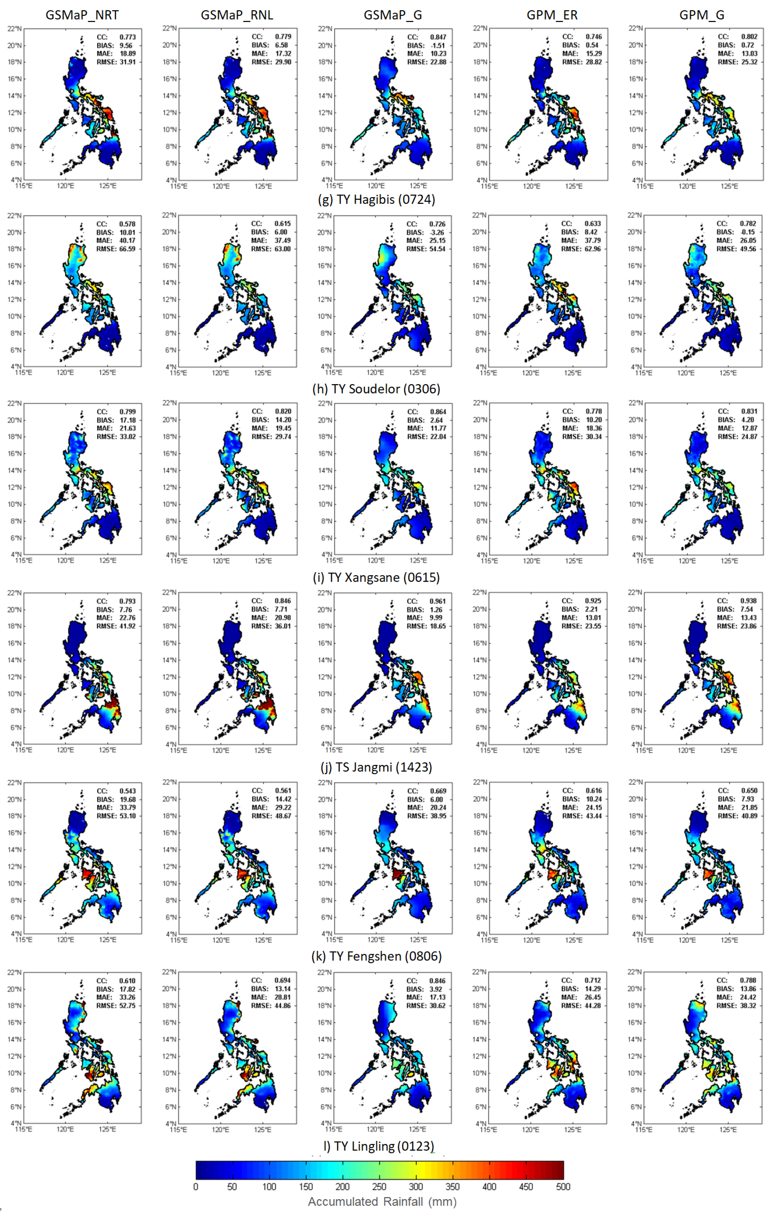
Figure 2 shows the TC rainfall distribution of selected TCs that are representative of most TC rainfall events. A total of 152 TCs that traversed within 5° of the Philippine landmass were selected for assessment. It is important to note that only the synoptic stations that were within 5° of the TC center were used in the rainfall estimation assessment. Figure 2a shows the rainfall from TY Kai-Tak (2000) which formed just off the west coast of Luzon Island. TY Kai-Tak slowly moved northward resulting in intense rainfall along the western section of Luzon. It is apparent that the rainfall amounts from GSMaP_NRT and GSMaP_RNL were considerably higher compared to the underestimated GPM_ER. The gauge-calibrated GSMaP_G and GPM_G show similar rainfall in terms of amount and distribution, however, there is a visibly high rain value around 16.5° latitude of western Luzon in the GSMaP_G. This location corresponds to the Baguio synoptic station. This station is distinctive as it is located 1500 m above sea level and is one of only two stations in the Philippines located in mountains. Basconcillo et al. [11] found that due to its location/altitude, Baguio station has high kurtosis when used in interpolated rainfall data, indicating that the station produces a high frequency of outlier observations. It may appear that GSMaP_G estimations are skewed towards ground observation values as indicated by the higher rainfall amounts around Baguio station, this is also observed in other TC events such as TY Mangkhut (Figure 2b), TY Parma (Figure 2c), TY Soudelor (Figure 2h), and several other TCs not shown here. TCs where there is high rainfall amount in Baguio station for GSMaP_G typically results in a lower spatial correlation value between stations compared to GPM_G.

Figure 2b shows the rainfall distribution from TY Mangkhut. TY Mangkhut was a category 5 system that caused widespread flooding and landslides across northern Luzon in September 2018 and is considered the 5th costliest TC in the country [32]. The GSMaP_NRT and GSMaP_RNL also overestimated the regions within 150 km of the TC track with high mean biases of 92.6 mm and 84.3 mm, respectively. GSMaP_NRT and GSMaP_RNL have systematically high biases in almost all TC events. A notable feature in the GSMaP_G rainfall for TY Mangkhut is the slightly lower rain amounts in the northeast Luzon region. This dry bias of GSMaP_G is also seen in TY Melor (Figure 2d), TY Ketsana (Figure 2e), STS Nock-Ten (Figure 2f), TY Hagibis (Figure 2g), TY Soudelor (Figure 2h), and TY Lingling (Figure 2l), or in events with significant rainfall in the northeast region. This is despite TY Mangkhut (Figure 2b), TY Parma (Figure 2c), and TY Melor (Figure 2d) having high rainfall in the northeast region for the other GSMaP and GPM rain estimations. The lack of station observations in that region likely produces this dry bias that is apparent in data interpolation, as described in the results of Bagtasa [3]. The GSMaP_G rain distribution has smooth features and seems to follow the appearance of interpolated rainfall data, which further reinforces the observation that GSMaP_G relies heavily on and is skewed towards ground observations.

Figure 2d shows the rain distribution of TY Melor. TY Melor was an intense, category 4 typhoon that affected the Philippines in December 2015. Its most intense rain was mostly to the east of Luzon, characteristic of late-season TCs [3]. GSMaP_G shows a significant dry bias along the northeast of Luzon compared to all other precipitation datasets. GSMaP_G dry bias is also seen in the southern portion of Mindoro Island, which is visible in almost all cases where considerable rainfall has fallen in that region (i.e., TY Ketsana in Figure 2e, STS Nock-Ten in Figure 2f, and TY Fengshen in Figure 2k). Another observation for the GSMaP_NRT and GSMaP_RNL seen in the TY Melor case is the uneven distribution or the presence of patches of extreme rainfall over Luzon. These patches are also observed in TY Parma (Figure 2c), TY Ketsana (Figure 2e), STS Nock-ten (Figure 2f), TY Hagibis (Figure 2g), TY Soudelor (Figure 2h), TY Xangsane (Figure 2i), and TY Lingling (Figure 2l). In almost all TC cases, the rain patches disappear in the calibrated version GSMaP_G. For GPM_ER, patches of high precipitation are also seen but to a lesser extent, and these patches do not necessarily disappear in the gauge-calibrated version GPM_G. GSMaP_G and GPM_G have similar rainfall distribution in the islands of Visayas and Mindanao with the uncalibrated versions generally showing wet biases (Figure 2f–l). The smoothing in GSMaP_G may not appear visibly apparent due to the smaller landmass in the central and southern Philippines. However, TC rainfall estimation from GSMaP_G along the island of Palawan appears to be systematically underestimated.

Figure 3 shows the spatial correlation coefficient, bias, MAE, and RMSE of the satellite rainfall datasets for all 152 TC events.

Table 3. Average correlation coefficient, bias, MAE, and RMSE of satellite rainfall estimation of GSMaP_NRT, GSMaP_RNL, GSMaP_G, GPM_EA, and GPM_G.

	GSMaP_NRT	GSMaP_RNL	GSMaP_G	GPM_ER	GPM_G
Correlation	0.632	0.667	0.790	0.725	0.771
Bias	17.756	14.812	1.335	4.900	4.037
MAE	28.966	25.978	12.511	17.850	15.324
RSME	52.736	48.577	25.448	32.559	28.962

Bold number denotes statistically highest score.

shows the mean values of the same statistical scores as in Figure 3. GSMaP_NRT and GSMaP_RNL have the lowest spatial correlation, highest bias, MAE, and RMSE among all datasets. These two datasets also have the most outliers with low scores. The GSMaP shows significant improvements in its gauge-calibrated GSMaP_G scoring the highest correlation and lowest bias, MAE, and RMSE among all datasets. In the case of GPM, GPM_G has improved scores relative to the GPM_ER but is still lower compared to the GSMaP_G. Using the one-tailed t-test shows the mean correlation coefficient of GSMaP_G has no statistical difference from that of GPM_G at p < 0.05, but GSMaP_G has a significantly lower bias, MAE, and RMSE compared to GPM_G.

GSMaP_G tends to have the least bias and errors (MAE and RMSE). It is also seen in the box plots that the bias and error scores of GSMaP_G have the least variance for all TC events. However, GSMaP_G also tends to appear smoothened, similar to how interpolated ground observations appear. As mentioned, this is likely due to the higher dependence of the GSMaP_G on ground observations rather than from the combined microwave-infrared satellite data. This also results in the loss of the orographic features seen in TC rainfall distributions [5,33]. However, due to the current limitations on the low-density network used for the validation, it is difficult to conclusively determine which between GSMaP_G and GPM_G has a better performance.

Figure 4 shows the temporal correlation coefficient at each synoptic station of the five satellite precipitation products. The uncalibrated GSMaP_NRT and GSMaP_RNL have very similar correlation coefficient values ranging from 0.12 to 0.81 and an average of 0.60 and 0.63, respectively. The stations along the central Philippines’ eastern region appear to have the highest correlation for GSMaP_NRT and GSMaP_RNL. The correlation coefficients significantly improved in the GSMaP_G version with values ranging from 0.40 to 0.95 and an average of 0.80. The GPM_ER has a better correlation compared to the uncalibrated GSMaP with values ranging from 0.21 to 0.87 and an average of 0.70 while the GPM_G correlation ranges from 0.36 to 0.94 averaging 0.75. Interestingly, some stations with lower correlation values in GSMaP_G appear to be better in the GPM_G. Overall, the mean temporal correlation values for GSMaP_G and GPM_G are statistically the same.

Figure 5 shows the contingency scores using the following rainfall threshold values: 0, 7.5, 15, 30, 50, 75, 100, 150, 200, 250, and 300 mm. Figure 5a shows the POD or hit rate of GSMaP_G and GPM_G datasets are above 60% for all rainfall thresholds, except the 200 mm threshold for GPM_G with POD of 0.58. The POD of the non-calibrated datasets gradually decreased with higher rainfall thresholds. Similarly, the PSS (Figure 5b) of GSMaP_G and GPM_G were almost constant with the thresholds taking values ranging 0.57–0.72. Figure 5c,d show the CSI and FAR, respectively. CSI or threat score decreases for more extreme rainfall from 0.8 for the rain/no-rain identification to 0.20 and 0.29 for GSMaP_G and GPM_G at the 300 mm rainfall threshold, respectively. The FAR scores in Figure 5d are similar for all rainfall products which increase with a higher rainfall threshold. The frequent overestimation of the uncalibrated datasets, especially for GSMaP, resulted in low FAR at higher rainfall thresholds.

To further understand the behavior of the statistical skill scores, Figure 6 shows the probability density function (PDF) histogram of the satellite rainfall estimates. All satellite products tend to overestimate the frequency of rain in the rain/no-rain identification. This is expected as the footprint of satellite grids is large enough to account for rainfall away from stations but still within the grid, Veloria et al. [10] found that rainfall 1 km away from synoptic stations, but still within the 0.1° by 0.1° satellite grid, can have significant differences. It is also noteworthy that the scores here are only for TC rainfall, all non-TC rainfall or rainfall outside of the 5° radius from a TC center was discarded. For light rain of 1–7.5 mm and 7.5–15 mm, the uncalibrated GSMaP products tend to underestimate their frequencies. However, since TC rainfall is the focus of this assessment, light rain is typically found outside the TC rainbands. Then, from 30 mm and higher rainfall, the two GSMaP datasets overestimated the occurrence frequency. The gauge-calibrated GSMaP and both uncalibrated and calibrated GPM behaved similarly throughout the different rainfall thresholds. GSMaP_G, GPM_ER, and GPM_G generally followed the PDF of the observation except for the rain/no-rain identification and the 15 mm to 50 mm bins where frequencies were slightly overestimated compared to the observed.

3.1. Discussion

TC rainfall estimation products from satellites can be very helpful in real-time quick assessment or post-analysis of flooding and the consequent damages from TCs. The near real-time GSMaP_NRT and the early GPM_ER both have low latencies of about 4 h that can be used in hydrological models for flood forecasting [34]. Both near-real-time datasets tend to overestimate TC rainfall as shown by their high biases, errors, and overestimated frequency for bins >30 mm. This high bias and frequency overestimation also led to relatively low FAR and low correlation coefficient values in many stations. The GPM_ER showed better scores overall compared to GSMaP_NRT and is deemed a better real-time satellite rainfall estimation product. The uncalibrated GSMaP_RNL is fractionally better than the GSMaP_NRT in almost all metrics but still has relatively lower scores than GPM_ER.

For the gauge-calibrated datasets, GSMaP_G has the highest statistical scores with the highest spatial and temporal correlation and the lowest bias and errors with the least variability between TC events. Contingency scores and PDF are comparable to that of GPM_G, but overall GSMaP_G is marginally better. There are vast improvements in skill scores from GSMaP_NRT to GSMaP_G, however, GSMaP_G appears to be smoothened to pull its values towards ground rainfall observations. This is likely why GSMaP_G scores the highest in this assessment. GPM_G is comparable with GSMaP_G but with slightly higher bias and errors but shows no statistical difference in terms of spatial correlation coefficient values. In addition, the smoothing seen in GSMaP_G is not apparent in GPM_G. Consequently, the orographic and land features are still perceptible in the spatial rainfall distribution of GPM_G.

3.2. Analog Forecasting

3.2.1. Training Phase

Analog forecasting of TC rain is done by creating a composite mean rainfall from rainfall of similar or analog past TCs. To produce a composite rain map of a target TC, each 6-hourly position of a target TC is matched with past TCs nearest to the target TC point, referred to as member TCs. The member TCs are arranged according to their distance from the location point of the target TC. Averaging the rainfall of the member TCs at the 6-hourly point produced composite rainfall, this is repeated for each of the 6-hourly location points within 5° of the landmass of the target TC. Based on the assessment results in the previous sections, GSMaP_G and GPM_G will be used in analog forecasting, hereafter referred to simply as GSMaP and GPM, respectively. Several sensitivity tests were performed to obtain an optimal set of TC members that will be used in the averaging. First, the sensitivity to the number of TC members was tested by varying the number of members from 1 to 40. In addition, the TC rain rate, hence the accumulated rain amount, is dependent on TC intensity [3,35]. To adjust for TC intensity, the rain from each TC member is adjusted to match the intensity of the target TC. To do this, TC minimum central pressure was divided into 8 bins of 15 hPa intervals: >1000 hPa, 1000–985 hPa, 985–970 hPa, 970–955 hPa, 955–940 hPa, 940–925 hPa, 925–910 hPa, and <910 hPa. Then, a composite of the mean rainfall within 5° of the landmass of all TCs falling within each of the bins was calculated. The mean TC rainfall for each bin follows a linear trend where TCs belonging to bins of lower minimum central pressure had higher mean rainfall given by the equation y = 2.9x + 16.6, where y is the mean rain and x is the bin number from 1 to 8 corresponding to the highest to lowest central pressure bin. TC rain of a member TC was adjusted by multiplying the ratio of the target TC mean rain and the member TC mean rainfall to match the intensity of the target TC. Also, it has been shown in previous studies [3,4] that the rainfall distribution of TCs varies with the monsoon season. Here, the southwest monsoon season is defined as the months of June to September [6] while northeast monsoon or easterlies are outside of those months.

All TCs from June 2000 to December 2018 were used for the sensitivity test to the number of TC members, TC intensity adjustment, and TC seasonality. Figure 7a,e shows the correlation coefficient, bias, MAE, and RMSE of the composite rain with varying TC members. The spatial correlation values decrease while bias and errors (MAE and RMSE) increase with the number of TC members. Figure 7b,f show the same statistical scores with adjustments according to TC intensity. It is apparent, regardless of which dataset is used, that bias and errors have smaller values and become independent of TC members. There is also a drop in correlation values for GSMaP for TC members of up to 18. In Figure 7c,g, only TC members belonging to the same season as the target TCs were used in creating the rain composite, which shows a slightly improved correlation coefficient. This is consistent with TC rain distribution dependence on monsoon season. Rainfall distribution becomes spatially more coherent when using member TCs in the same season as the target TC. However, seasonality does not seem to affect the values of bias and errors. Lastly, Figure 7d,h show both adjustments in TC intensity and seasonality result in improvements in correlation coefficient, bias, and error values. The correlation coefficient of GSMaP with fewer members seems to behave differently from that of GPM rain composites. From the result, composites of 10 members are chosen to be the optimal as it is more or less the single value of members that can be applied to both datasets in the analog TC rain forecasting.

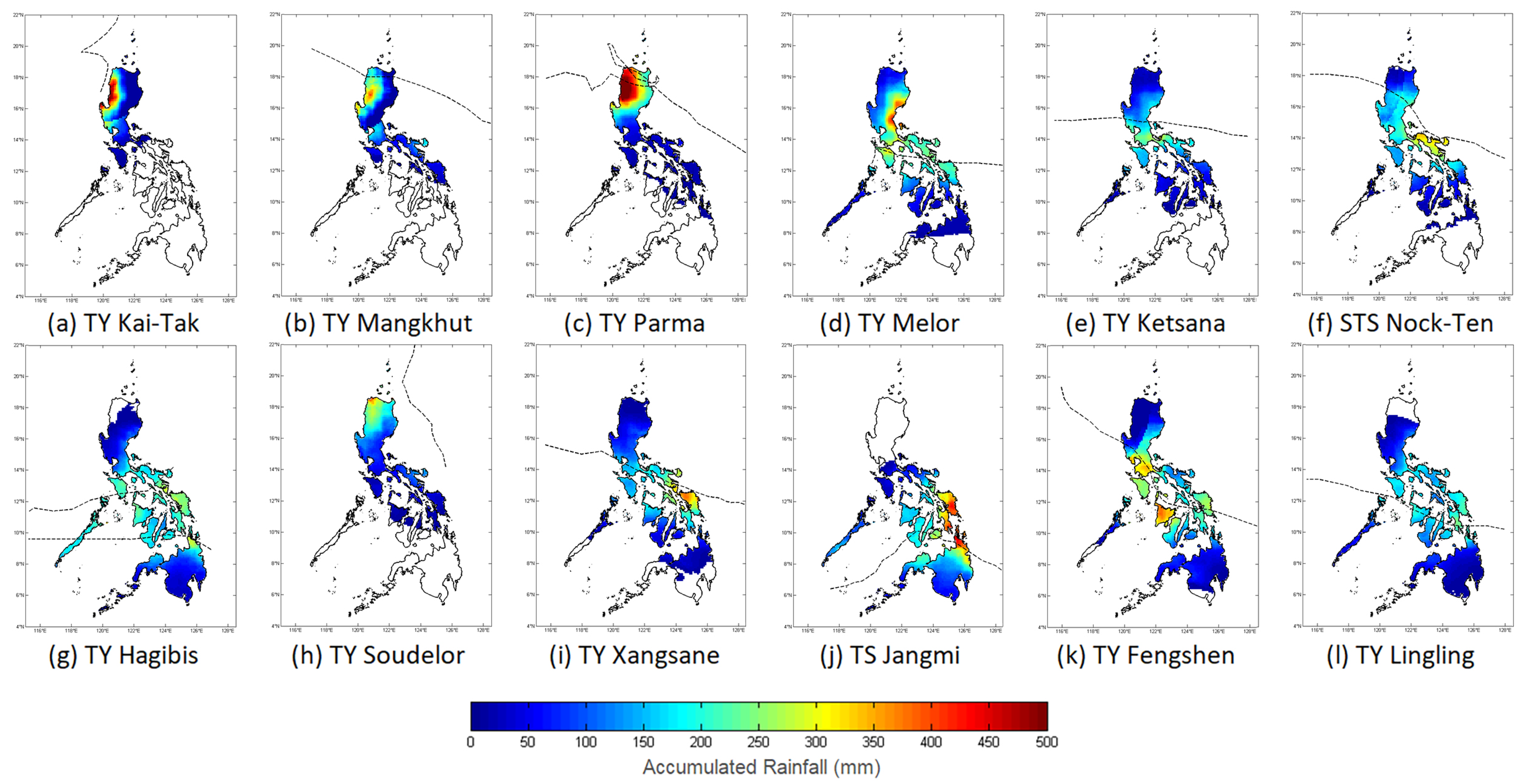
Figure 8 and Figure 9 show the distribution of the 10 member-composite target TC rainfall using the selected TCs shown in Figure 2 for GSMaP and GPM, respectively. Overall, the analog rainfall composites captured the TC rain distribution of the GSMaP_G and GPM_G estimates of TCs as in the cases of TY Kai-Tak (Figure 8a and Figure 9a), TY Mangkhut (Figure 8b and Figure 9b), TY Parma (Figure 8c and Figure 9c), TY Xangsane (Figure 8i and Figure 9i), and TS Jangmi (Figure 8j and Figure 9j). The composite for TY Mangkhut (Figure 8b and Figure 9b) using GSMaP_G also shows the high rain amount around Baguio station, which implies that the area is systematically overestimated to still appear in the composite mean. This station bias did not appear with the use of GPM_G. Some rain distributions are spatially shifted such as in the case of TY Parma (Figure 8c and Figure 9c) and TY Soudelor (Figure 8h and Figure 9h), which mainly results from the differences in the rain distribution of member TCs. An underestimation of peak rain in the eastern coastal regions of southern Luzon and Visayas is observed in STS Nock-Ten (Figure 8f and Figure 9f), TY Hagibis (Figure 8g and Figure 9g), and TY Soudelor (Figure 8h and Figure 9h), and around the western Visayas in TY Fengshen (Figure 8k and Figure 9k) and TY Lingling (Figure 8l and Figure 9l). This dry bias is likely due to the smoothing that arises from averaging the TC members, overall bringing down the peak rainfall values. This is also likely what occurred in the case of TY Ketsana (Figure 8e and Figure 9e), which was only a TS when it traversed Luzon but brought a 150-year return period rainfall [36]. Its composite rain is shown in Figure 8e and Figure 9e show lower rainfall than observed but still resembles the overall distribution.

3.2.2. Testing Phase

Using the optimal 10-member value in producing composite means together with TC intensity and seasonality adjustments, rainfall composites were produced for the 2019–2021 TCs using rainfall data from the training dataset (2000–2018).

Table 4. Mean TC rain forecast skill score from testing dataset TC (2018–2021): spatial correlation, bias, MAE, and RMSE.

	Correlation	Bias	MAE	RMSE
GSMaP	0.620	−13.26	35.07	57.21
GPM	0.669	−5.02	33.15	53.09

Bold number denotes statistically highest score.

summarizes the statistical scores of the analog TC rain forecasts. Analog forecasting using the GPM dataset yields statistically higher values in all statistical scores, except for MAE where no statistical difference was found between using GPM or GSMaP. In addition, the values of correlation, bias, and RMSE of the analog forecasts using either dataset show better scores than the assessment of the uncalibrated GSMaP_NRT and are comparable to the assessment skills of GSMaP_RNL or GPM_ER. This implies that analog forecasts can be used in both short-term forecasts, assuming that available track forecasts have minimal errors and real-time monitoring applications.

Figure 10 shows the contingency scores (POD, CSI, PSS, and FAR) of the analog forecasts of the testing TCs at different rainfall thresholds. The POD of both datasets shows values generally ranging from 0.9 in the rain/no-rain identification to 0.7 for 200 mm rainfall. PSS shows positive values up to the 200 mm threshold indicating skill in predicting different rainfall amounts. The analog TC rain predictions have CSI values of around 0.9 in the rain/no-rain identification but suddenly decline to about 0.5 at the 15–100 mm threshold and to 0.4 at the 200 mm threshold for GSMaP and a nearly constant value of 0.6 for GPM at the same threshold value. FAR steadily increases with a value of 0.1 in the rain/no-rain identification to more than 0.9 in the 200 mm threshold. Furthermore, there are no contingency scores past 200 mm due to the small number of observations with more than 250 mm matching the forecasts, which makes the estimated contingency scores inconclusive. The analog composite rainfall also appears to be “smoothened” due to the averaging of many members resulting in the inability to catch very intense rainfall, similar to the results of the composite analog TC rainfall forecasts in Bagtasa [3]. This averaging down of extreme rainfall can be addressed by other means such as artificial neural networks [37,38], but is outside the scope of this study. Another limitation of analog forecasting is the frequent occurrence of unprecedented weather events, such as those that are caused by climate change. Delfino et al. [32] showed that warming air and sea surface temperatures will likely increase the precipitation carried by TCs affecting the Philippines. However, the projected increases in precipitation depend on various factors (i.e., TC location, the intensity of warming, environmental conditions, etc.) that it is impossible to address in a simplified analog forecasting method such as what is presented here. Dynamical TC rain forecast models remain to be computationally expensive. The main goal of exploring analog TC rain forecast methods like the one presented in this study is to create a simple method of forecasting TC rain that can be utilized more as an auxiliary to existing global models rather than as a primary forecasting tool.

4. Summary and Conclusions

The aim of the present study is twofold, (1) to assess satellite precipitation products of GSMaP and GPM for TC rainfall, and (2) to use the precipitation estimates in analog forecasting of TC rainfall in the Philippines. TC rainfall is important in supplying water to reservoirs but also poses a great hazard that can lead to disastrous consequences. Two satellite precipitation datasets were assessed in this study, namely GSMaP and GPM. The datasets were selected as they are currently the two datasets with the highest temporal and spatial resolution. Moreover, several precipitation estimation algorithms were used for each of the datasets. The uncalibrated near-real-time GSMaP_NRT and reanalysis GSMaP_RNL, the gauge-calibrated GSMaP_G for GSMaP, the uncalibrated early version GPM_ER and the gauge-calibrated GPM_G for GPM. The near-real-time and the early versions have latencies of about 4 h, making them ideal for TC rain monitoring and/or quick damage assessment applications.

The uncalibrated GSMaP_NRT scored the lowest in statistical and contingency skill scores, followed by GSMaP_RNL. Both rainfall estimates have the lowest correlation coefficient and highest bias, MAE, and RMSE, with POD, PSS, and CSI constantly decreasing for higher rainfall thresholds. However, they have the lowest FAR for intense rainfall due mainly to their systematic overestimation. The early version GPM_ER performs better than GSMaP_NRT and GSMaP_RNL with less overestimation. There are slight improvements in all skill scores for the calibrated GPM_G compared to GPM_ER, but the highest overall performance belongs to GSMaP_G, not only scoring the highest in the assessments but doing so with the least variability among the TC events assessed. The drawback, however, of GSMaP_G is that rain distribution appears to be spatially smoothened to follow the gauge-observed rainfall values, giving it the highest assessment scores but appears to lose the orographic features in the rainfall distributions.

The satellite precipitation estimates of GSMaP_G and GPM_G were then utilized in the analog forecasting of TC rainfall. TC rainfall forecasts of target TCs are done by creating a composite mean rainfall from rainfall of similar or analog past TCs. This is done by getting the 6-hourly location point of a target TC, then, searching all past TCs according to their distance to the target TC location. The rainfall of the closest analog TC points was then averaged. To determine the optimum number of analog member TCs to be included in the averaging, TC members were varied from 1 to 40. In addition, the rainfall of member TCs was individually adjusted to match the intensity of the target TC and only member TCs belonging to the same monsoon season were included as analogs. The determination of optimum TC members was gathered from a training dataset that comprise landfalling TCs from 2000 to 2018. Results show that statistical skill scores were generally independent of TC members. It was decided that a 10-member composite will be used in the testing dataset which includes all landfalling TCs from 2019 to 2021. The analog forecasts generally captured the spatial distribution of TC rainfall with statistical skill scores faring better than the uncalibrated GSMaP_NRT dataset, indicating acceptable forecast skills.