Abstract
As a key parameter of land surface energy balance models, near surface air temperature (NSAT) is an important indicator of the surface atmospheric environment and the urban thermal environment. At present, NSAT data are mainly captured by meteorological ground stations. In areas with a sparse distribution of meteorological stations, however, it is not possible to describe the heterogeneity of NSAT in continuous space. With the rapid development of satellite remote sensing technologies, there is now a significant method to retrieve NSAT from multispectral satellite images based on machine learning methods. In the literatures published so far, there is little reported research concerning the comprehensive evaluation and/or the systematic comparison of NSAT retrieval performances based on different machine learning models. Hence, the three most commonly-used machine learning models, Support Vector Regression (SVR), Multilayer Perceptron Neural Network (MLBPN), and Random Forest (RF), have been employed for the NSAT retrieval from various multispectral satellite images of MODIS daytime and nighttime data, Landsat 8 data, and Sentinel-2 data. Comparison of the NSAT retrieval results generated by the different machine learning models from the different types of satellite images reveals that (a) the RF-based model has a better NSAT retrieval performance than the SVR- or MLBPN-based models with respect to both the accuracy and stability, and (b) the NSAT results retrieved from the MODIS data were generally better than those from the Landsat 8 and Sentinel-2 data. To sum up, the conducted research in this article does not only provide a reference for practical applications relevant to NSAT retrievals, but also proposes an efficient RF-based model for NSAT retrieval from multispectral satellite images in continuous space.
1. Introduction
As a key parameter of land surface energy balance models, near surface air temperature (NSAT) is not only an important indicator of the surface atmospheric environment and the urban thermal environment but is also a significant parameter of land surface energy balance models [1,2,3]. Because various land surface processes, such as photosynthesis and respiration, are affected by NSAT, the continuous spatial distribution of the NSAT with suitable temporal and spatial resolution is necessitated by various studies concerning land–surface modelling, global environmental changes, urban heat island effect, etc. [4,5]. At present, NSAT data are primarily captured by meteorological ground stations. With the successful launching of various multispectral satellite sensors, including MODIS, Landsat, Sentinel, etc., satellite remote sensing technology has become one of the most efficient ways to acquire NSAT data with high temporal and/or spatial resolution. Five methods have been widely employed to retrieve the NSAT data from multispectral satellite images in recent decades: the single-factor method, multi-factor method, temperature vegetation index (TVX) method, surface energy balance method, and machine learning method.
1.1. The Single-Factor Method
The single-factor method can be used to analyze the correlation between NSAT and Land Surface Temperature (LST) based on a linear regression model [4]. The correlation coefficients (R2) between the LST extracted from satellite data and the NSAT measured by on-site monitors exceeded 0.95 in the experiments conducted by Basist et al. [6]. Fu et al. used LST provided by MODIS to retrieve NSAT in the northern Qinghai-Tibet Plateau based on a linear regression model, and they found that the daily NSATmin (minimum NSAT) and the nighttime NSATavg (average NSAT) can be retrieved in cases where the input LST data are accurate [7]. In a paper by Zhang et al., the NSAT results retrieved from nighttime LST provided by MODIS were generally better than those from daytime LST [8]. Although the single-factor method has been widely employed by many researchers for NSAT retrieval, the accuracy and stability of this method are highly dependent on the time, location, and amount of the observational data.
1.2. The Multi-Factor Method
As an upgrade to the single-factor method, the multi-factor method has been developed and employed by researchers to improve the retrieval accuracy and enhance its usability. Based on this method, Cresswell et al. used the temperature of Meteosat and the Solar Zenith Angle (SZA) to retrieve NSAT, with an accuracy of 3 °C for over 70% of the data [9]. Zhao et al. found that the linear regression model with monthly average LST, elevation, and topographic factors outperformed the three statistical methods of spline, inverse distance weight, and kriging [10]. Xu et al. developed a statistical model to retrieve NSAT using LST, elevation, Normalized Difference Vegetation Index (NDVI), and albedo as inputs [11]. In general, the accuracy of the multi-factor method is better than the single-factor method, while the accuracy and stability are still limited by the time, location, and amount of the observational data.
1.3. The Temperature Vegetation Index Method
Like the single- and multi-factor methods, the temperature vegetation index (TVX) method can also be employed for NSAT retrieval, based on the negative correlation between the atmosphere temperature and spectral vegetation index [12]. With the observed LST and the NDVI, for instance, Prihodko and Goward et al. implemented the TVX method to retrieve the NSAT—the R² reached 0.93 and the Mean Error (ME) was 2.92 °C [13]. Nieto et al. compared the accuracy between the previous maximum NDVI (NDVImax) and the current NDVImax, which used the observed NSAT to calibrate the NDVImax for each vegetation type [14]. Zhu et al. improved the TVX method by lowered the threshold of the negative correlation coefficient of NDVI, which revealed the result with RMSE from 7.45 °C to 3.79 °C, the MAE from 6.21 °C to 3.03 °C, and R² equal to 0.83 [15]. However, the TVX method is unsuitable in areas with low vegetation and bare soil.
1.4. The Surface Energy Balance Method
In the research conducted by Pape et al., the surface energy balance model was established to simulate the LST and NSAT changes in a high temporal resolution alpine region, based on the measured NSAT and satellite remote sensing data [16]. Analogously, Hou et al. proposed an Energy Balance Bowen Ratio model to retrieval the NSAT from Landsat 5 TM images in Beijing, where the ME of the retrieval result was equal to 2.21 °C [17]. The surface energy balance method has been implemented in various regions and has revealed satisfactory results in cases where sufficient amounts of observation data were available.
1.5. Machine Learning Methods
Since the 2010s, more and more researchers have started to employ machine learning methods for the task of NSAT retrieval. For instance, Xu et al. employed the Random Forest (RF) model to retrieve maximum NSAT (NSATmax) from MODIS data in British Columbia, which revealed that the RF model had higher accuracy than the linear regression method [18]. Similar to Xu et al., Ho et al. found that the NSAT retrieval results based on the RF model were generally better than the ordinary least squared regression and the support vector machine models [19]. Based on the M5 model, Emamifar et al. retrieved the NSAT in Khuzestan province in southwestern Iran, with the LST calculated from MODIS, solar radiation, and Julian day as inputs. The results showed that the RMSE was 2.3 °C and the R² reached 0.96 [20]. In the MBR-LST model proposed by Zhang et al., the back-propagation neural network was employed to retrieve the land surface temperature (LST) based on the inputs of the band reflectance from Landsat 8 OLI/TIRS images, NDVI, elevation, latitude, meteorological parameters, and time parameters, which revealed a significantly better performance than the traditional Radiative Transfer Equation (RTE) method [21].
The reported work mentioned above indicates that satellite remote sensing technology, together with the proper machine learning methods have become an efficient way for the retrieval of NSAT in continuous space. In the literatures published so far, however, there are few studies concerning the comprehensive evaluation and/or systematic comparison of the NSAT retrieval performance of the various machine learning models. Hence, the three most commonly-used machine learning models in the environmental field, Support Vector Regression (SVR), Multilayer Perceptron Neural Network (MLBPN), and Random Forest (RF), have been employed for NSAT retrieval from the various multispectral satellite images of MODIS daytime and nighttime data, Landsat 8 data, and Sentinel-2 data. By comparing the NSAT retrieval results generated by the different machine learning models, the ‘optimal’ NSAT retrieval model, together with the ‘best’ satellite data as inputs will be sufficiently investigated in this research.
2. Study Area and Data Sources
2.1. Study Area
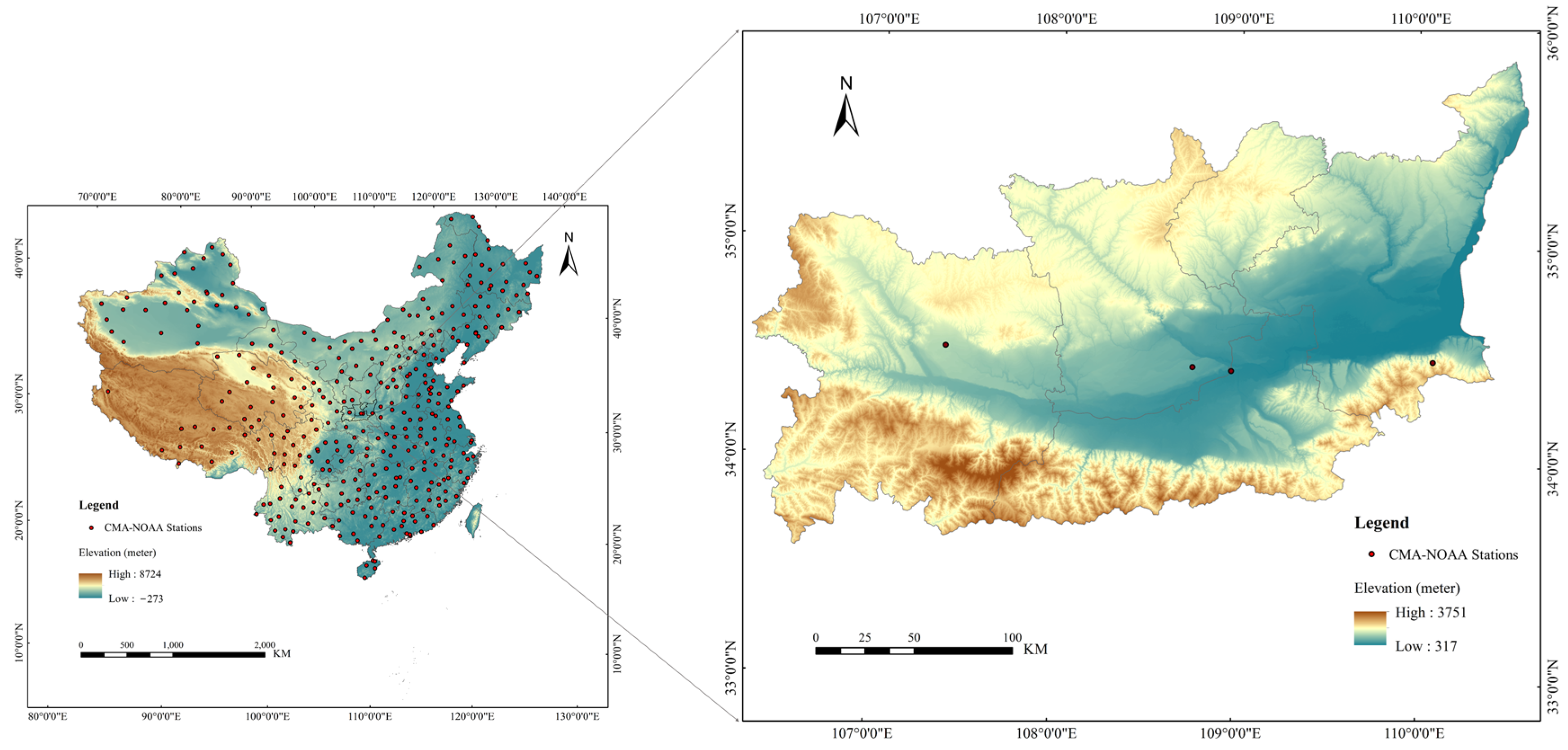
The Guanzhong area has been selected as the study area in this article and is located in the central part of Shaanxi Province between latitude 33°39’ N to 35°52’ N, and longitude 106°56’ E to 110°22’ E, with an area of 55,500 square kilometers.
As illustrated in Figure 1, the Guanzhong area is surrounded by the Qinling Mountains to the south, the Loess Plateau to the north, and the Weihe River Plain in the center. The Guanzhong area includes five cities, Xi’an, Baoji, Xianyang, Weinan, and Tongchuan, and it has a total population of more than 20 million and a warm temperate continental monsoon climate with an average annual temperature of 12 °C to 14 °C and an average annual rainfall of 500–700 mm. The Weihe River runs through the central part of the plain from west to east and joins the Yellow River from Tongguan [22,23].
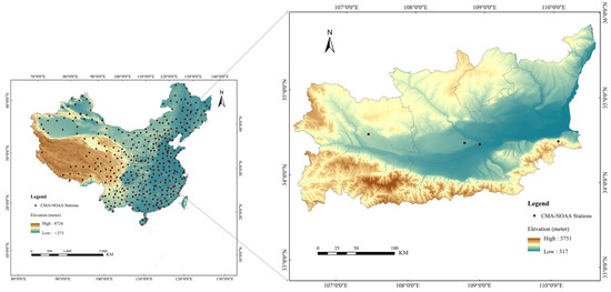
Figure 1.
Study area and distribution of CMA-NOAA stations.
2.2. Data Sources
2.2.1. MODIS Data
MODIS data were captured by the Terra and Aqua satellites, including 36 spectral bands from 0.4 μm (visible light) to 14.4 μm (thermal infrared), with spatial resolutions from 250 m to 1000 m. The revisit cycle in mainland China is 1–2 times/day. In addition to MODIS raw data, there are different categories of data products that can be downloaded for free [24]. This study used daily land surface temperature product (MOD11A1) captured at daytime (MODISTD) and nighttime (MODISTN), and daily surface reflectance product (MOD09GA) from 2010 to 2021.
2.2.2. Landsat 8 OLI Data
The Landsat 8 satellite was launched by National Aeronautics and Space Administration (NASA) on 11 February 2013, and it has two sensors, including an Operational Land Imager (OLI) and a Thermal Infrared Sensor (TIRS). Landsat 8 is mainly consistent with Landsat 1–7 in terms of spatial resolution and spectral characteristics, and it can achieve global coverage every 16 days [25]. In this study, the Landsat 8 images from 2013 to 2021 in the Guanzhong area were chosen as the original data.
2.2.3. Sentinel-2 Data
The “Sentinel” series of satellites are dedicated satellites of the European “Copernicus” Earth Observation Program. Sentinel-2 consist of Sentinel-2A and Sentinel-2B, which carry MSI imaging sensors with 13 bands from the visible light band to the shortwave infrared band. The spatial resolutions are 10 m, 20 m, and 60 m, respectively, and the revisit period of one satellite is 10 days [26]. This study used Sentinel-2A images captured from 2018 to 2021.
2.2.4. CMA-NOAA Data
The National Oceanic and Atmospheric Administration (NOAA) is the governing body for weather operations in the United States. In 2013, the China Meteorological Administration (CMA) signed a cooperation agreement with NOAA, authorizing NOAA to publicly publish meteorological data for mainland China on the Internet, termed as CMA-NOAA data. The CMA-NOAA data is published every three hours and mainly includes atmospheric pressure, humidity, temperature, wind direction, wind speed, etc. The dependent variable used in this study is NSAT data from CMA-NOAA, which applies to NSAT retrieval rather than LST retrieval. There are 372 CMA-NOAA stations in mainland China, including four stations in this study area (Figure 1).
2.2.5. SRTM-DEM Data
NASA and the National Imagery and Mapping Agency (NIMA) jointly completed the Shuttle Radar Topography Mission (SRTM). SRTM terrain data can be divided into SRTM1 and SRTM3, according to the spatial resolution [27]. In this study, SRTM1 data were used as the elevation of the study area. A total of 14 SRTM1 DEM 30 m images were obtained (Figure 1).
As illustrated in Table 1, there are four primary data groups employed by the proposed models. The remote sensing images data come from the GEE, the elevation data come from the USGS, and the measured NSAT data come from the CMA-NOAA meteorological ground station.

Table 1.
List of the primary data employed by the proposed models.
2.3. Data Preprocessing
Because the sample data are from different sources, the format and distribution characteristics of the data could be different to one another. Therefore, the sample data need to be preprocessed before applications, which can be characterized by the following two steps.
- (1)
- Removing the sample data heavily affected by clouds using the quality control tools provided by GEE. With the MODIS data, the data with QC larger than 0 were deleted, and a total of 1342 MODISTD samples and 1489 MODISTN samples were retained. With the Landsat 8 data, a total of 284 samples with BQA equal to 2720 were obtained. With the Sentinel-2 data, a total of 556 samples with QA60 equal to 0 were selected for further processing.
- (2)
- Satellite remote sensing images, temporal parameters, geo-spatial parameters, and the measured NSAT from ground stations were matched. In this way, the links between different sample data can be established so that the data from different sources can be fused together.
3. Methods
3.1. Support Vector Regression (SVR)
Support Vector Machine (SVM) is developed on the basis of statistical learning theory, which was proposed by Vapnik in the 1990s [28,29]. According to different applications, SVM is divided into Support Vector Classification (SVC) and Support Vector Regression (SVR). The theory of SVR is Structural Risk Minimization (SRM) rather than Empirical Risk Minimization (ERM). SVR can map the samples to high-dimensional space through the nonlinear mapping function, and can then use the kernel function to replace the vector inner product in high-dimensional space [29]. The Radial Basis Function (RBF) was chosen in this study. The formula is as follows [30]:
In this study, the retrieval accuracy of SVR mainly depends on C (Penalty Coefficient) and gamma. C represents the tolerance of model error. Gamma determines the distribution of the data after mapping to the new feature space.
3.2. Multilayer Perceptron Neural Network (MLBPN)
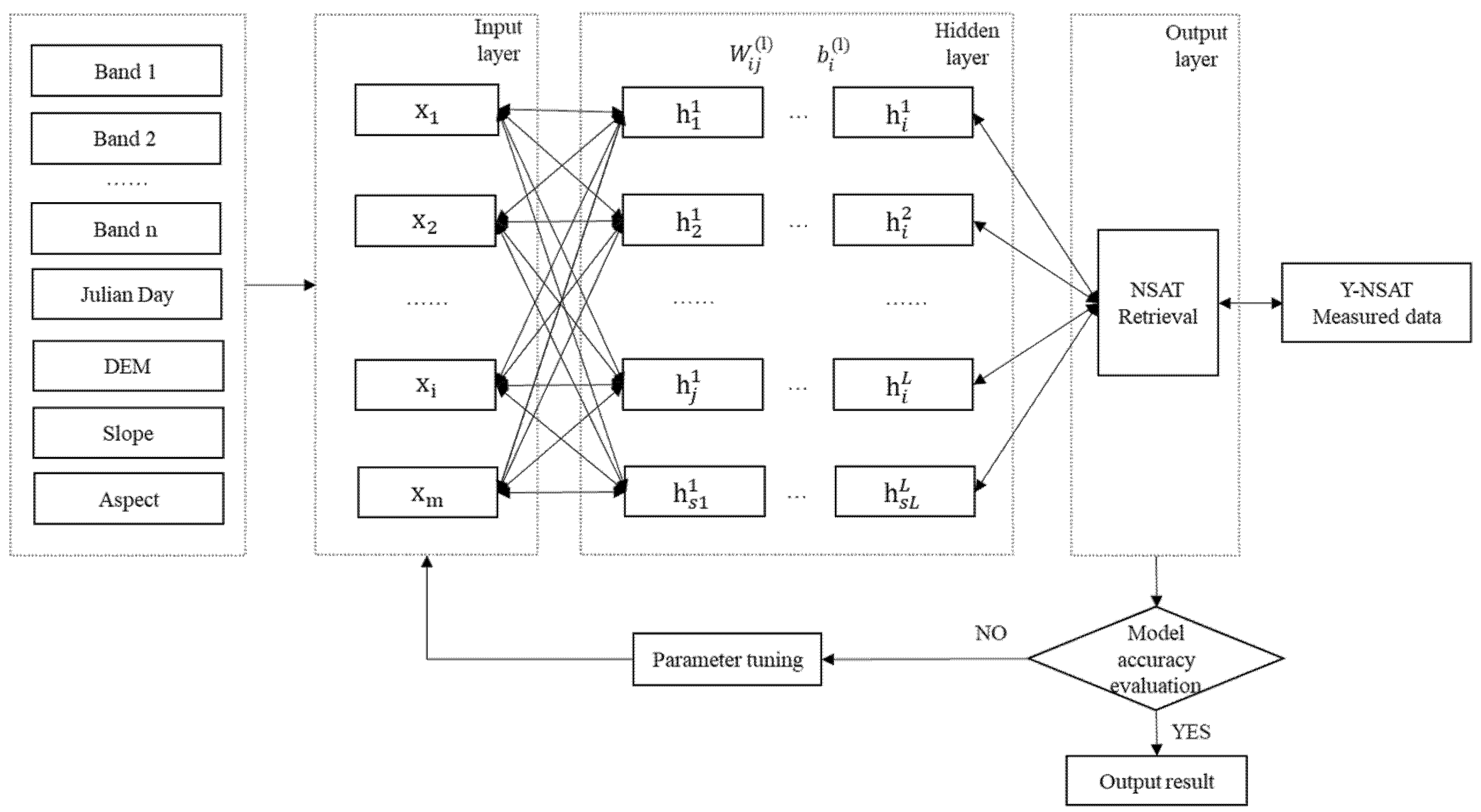
The Multilayer Perceptron Neural Network (MLBPN) model is based on an artificial neural network (ANN) [21]. The established MLBPN model is composed of one input layer, several hidden layers (L), and one output layer (see Figure 2). All the cells in the adjacent layers are connected to each other, while the cells of the same layer do not have any connection. represents the input vector, sl is the number of neurons in layer l, and hl = . Y is the output vector recording the NSATs derived from CMA-NOAA stations, is the connection weight between the jth neuron in layer l − 1 and the ith neuron in layer l, and is the bias of the ith neuron in the layer l. represents the input value of the ith neuron in the l layer and is the transfer function. The Tansig function is utilized for transmitting the neurons between different hidden layers [31], and the Purelin function is employed as the transfer function of the output layer [32,33].
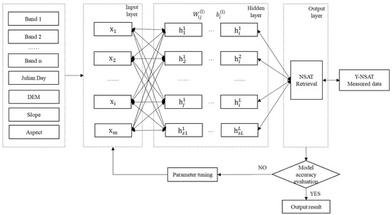
Figure 2.
Diagram of the multilayer perceptron neural network (MLBPN).
3.3. Random Forest (RF)
Random Forest (RF) was developed by Leo Breiman and Culter Adele in 2001 [34]. RF combines multiple decision trees into a decision tree forest, which is a new type of machine learning technology that can perform classification and regression analysis. The accuracy of RF is determined by each decision tree.
The Random Forest Regressor in scikit-learn is used for NSAT retrieval. The accuracy of the RF model depends on three important parameters: n_estimators (the number of trees in RF), max_depth (the maximum depth of tree in RF), and max_features (the maximum number of features to consider when dividing each tree in RF). In the optimization stage, the three parameters can be adjusted to improve the accuracy of the NSAT retrieval.
3.4. Validation
In this study, in spite of the data from the multispectral satellite images, the geospatial parameters, together with the time parameters, have been also considered to enhance the accuracy of the NSAT retrievals. To evaluate the NSAT retrieval accuracy of the three models, the following four statistical indicators of regression fitting determination coefficient (R2), Root Mean Square Error (RMSE), Mean Absolute Error (MAE), and Mean Error (ME) are employed.
where n is the number of samples, is the measured NSAT of the ith sample, and is the retrieved NSAT of the ith sample.
4. Results
4.1. Model Performance
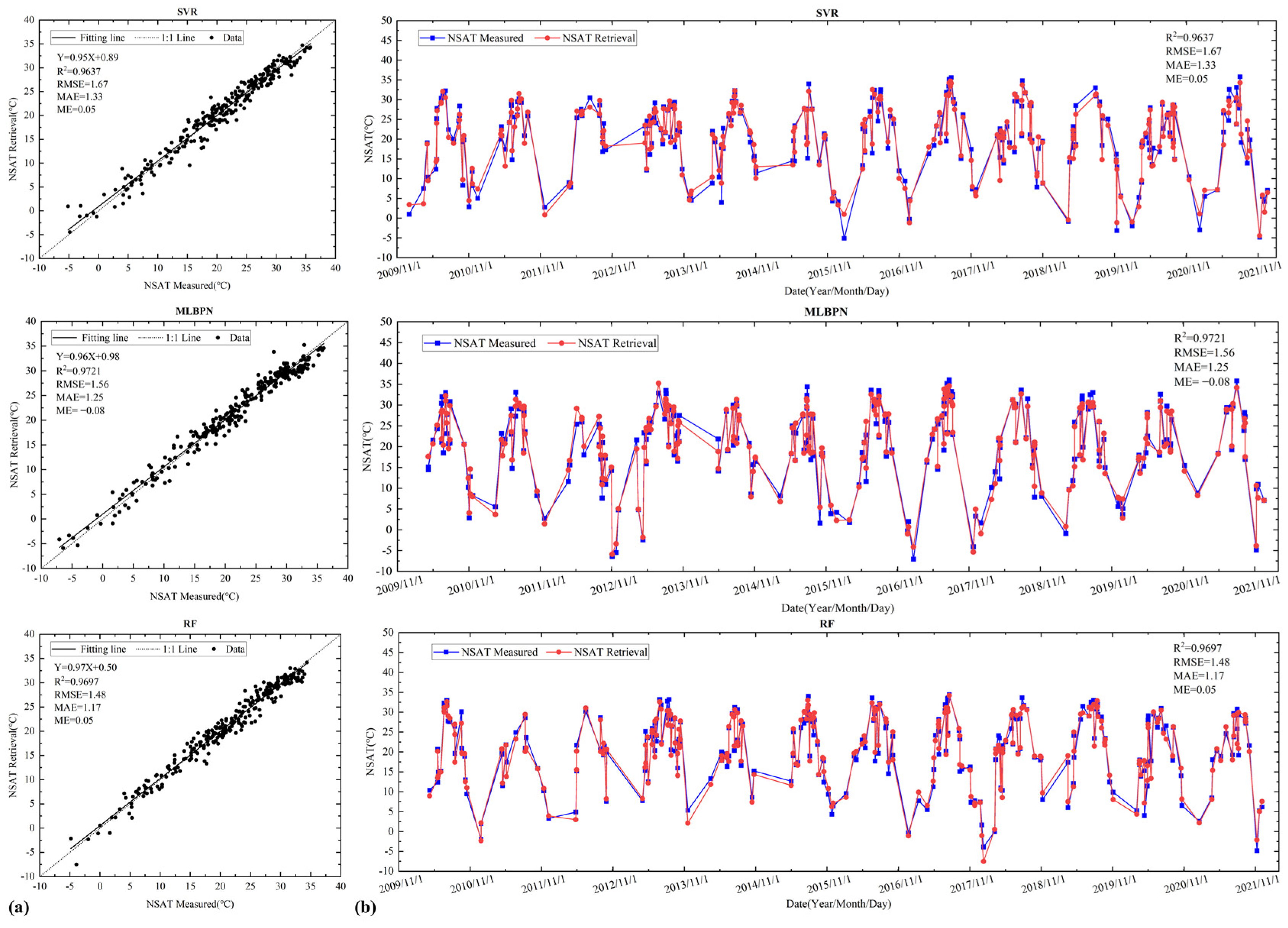
Figure 3 compares the measured NSATs from the ground observation stations with the retrieved values from MODISTD data, based on the SVR, MLBPN, and RF models, respectively. The R2 of the regression line based on all three models are close to 1 (see Figure 3a). To further analyze the accuracy of the retrieved NSATs, several samples (number = 269) captured from 2010 to 2021 have been randomly selected from all the collected data. The retrieved and measured values were then compared to one another (see Figure 3b). With the SVR-based model, the R2, RMSE, MAE, and ME are respectively equal to 0.9635, 1.70 °C, 1.31 °C, and 0.20 °C. With the MLBPN-based model, the R2, RMSE, MAE, and ME are 0.9721, 1.56 °C, 1.25 °C, and −0.08 °C. Compared to the SVR and MLBPN-based models, the RF-based model reaches an overall better NSAT retrieval results, with R2, RMSE, MAE, and ME equal to 0.9697, 1.48 °C, 1.17 °C, and 0.05 °C, respectively (see Table 2).
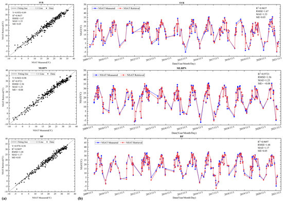
Figure 3.
Comparison between the measured and retrieved NSATs from MODISTD data: (a) Scatterplots of the measured and retrieved values, where the solid line is the fitting line obtained by line regression and the dashed line is the reference of y = x. (b) Measured NSATs (blue line) versus retrieved NSATs (red lines) of the randomly selected samples from 2010 to 2021.

Table 2.
Accuracy evaluation of the proposed NSAT retrieval models.
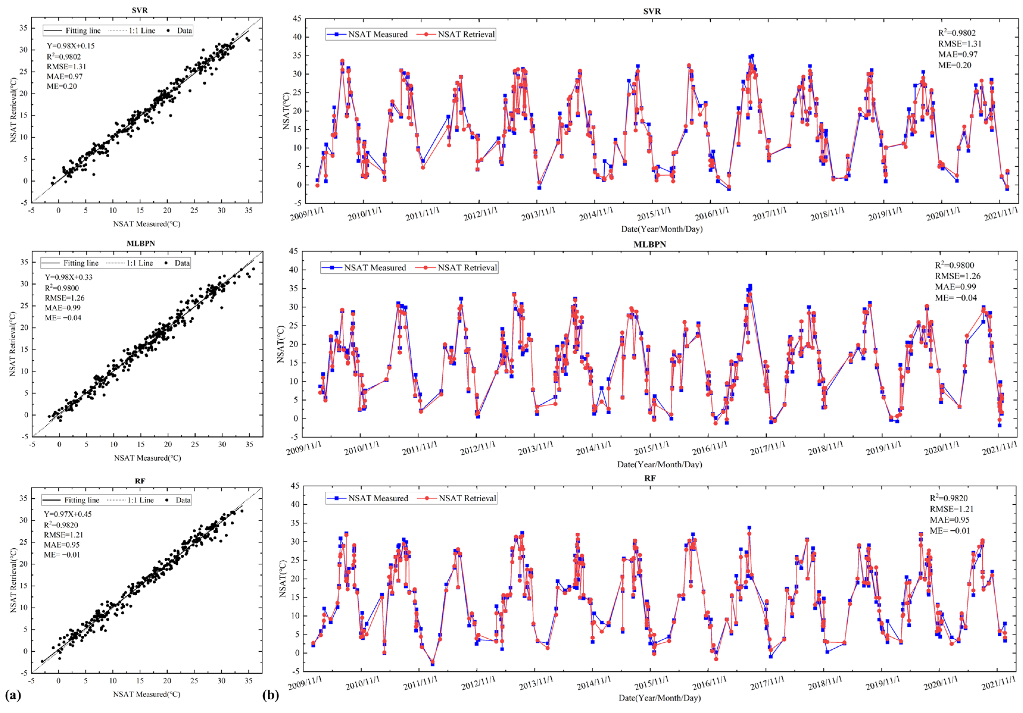
Figure 4 compares the results of the measured NSATs from the ground observation stations with the retrieved values from MODISTN data, based on the SVR, MLBPN, and RF models, respectively. All the R2 based on the three models are close to 1 (see Figure 4a). In Figure 4b, several samples (number = 298), captured from 2010 to 2021, have been randomly selected for further analysis. With the SVR-based model, the R2, RMSE, MAE, and ME are, respectively, equal to 0.9802, 1.31 °C, 0.97 °C, and 0.20 °C. With the MLBPN-based model, the R2, RMSE, MAE, and ME are 0.9800, 1.26 °C, 0.99 °C, and −0.04 °C. Compared to the SVR and MLBPN-based models, the RF-based model has revealed comprehensively better NSAT retrieval result, with R2, RMSE, MAE, and ME equal to 0.9820, 1.21 °C, 0.95 °C, and −0.01 °C, respectively (see Table 2).
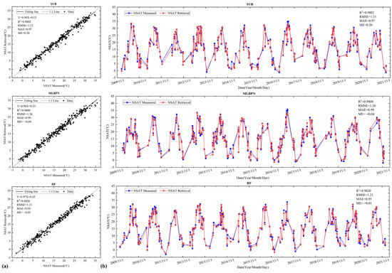
Figure 4.
Comparison between the measured and retrieved NSATs from MODISTN data: (a) Scatterplots of the measured and retrieved values, where the solid line is the fitting line obtained by line regression and the dashed line is the reference line of y = x. (b) Measured NSATs (blue line) versus retrieved NSATs (red lines) of the randomly selected samples from 2010 to 2021.
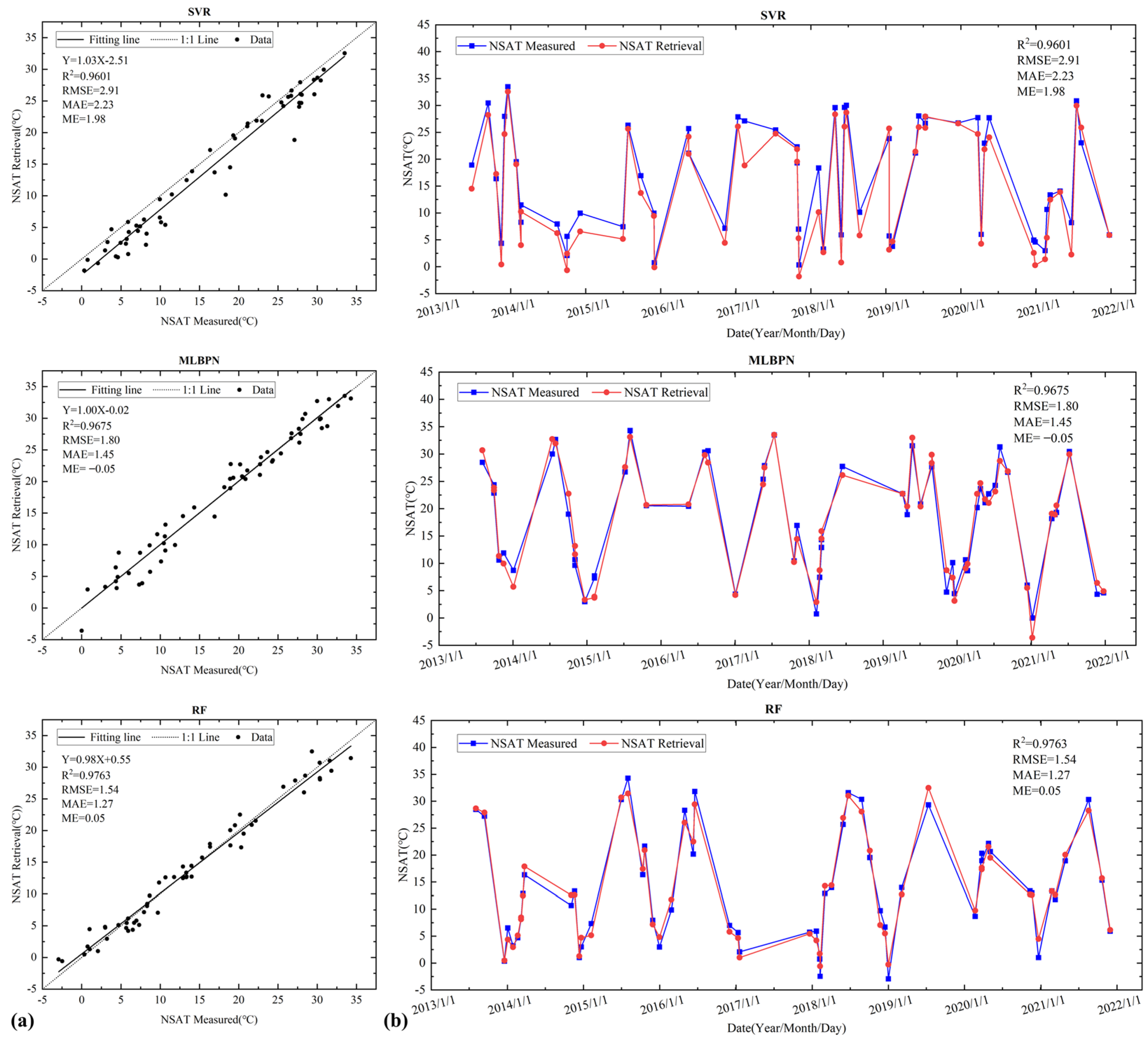
Figure 5 compares the measured NSATs from the ground observation stations with the retrieved values from Landsat 8 data. The R2 of the regression lines based on MLBPN and RF models are close to 1 (see Figure 5a). In Figure 5b, several samples (number = 57) captured from 2013 to 2021 have been randomly selected for further analysis, where the RF-based model reaches the best NSAT retrieval result with R2, RMSE, MAE, and ME equal to 0.9763, 1.54 °C, 1.27 °C, and 0.05 °C (see Table 2).
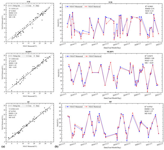
Figure 5.
Comparison between the measured and retrieved NSATs from Landsat 8 data: (a) Scatterplots of the measured and retrieved values, where the solid line is the fitting line obtained by the line regression and the dashed line is the reference line of y = x. (b) Measured NSATs (blue line) versus retrieved NSATs (red lines) of the randomly selected samples from 2013–2021.
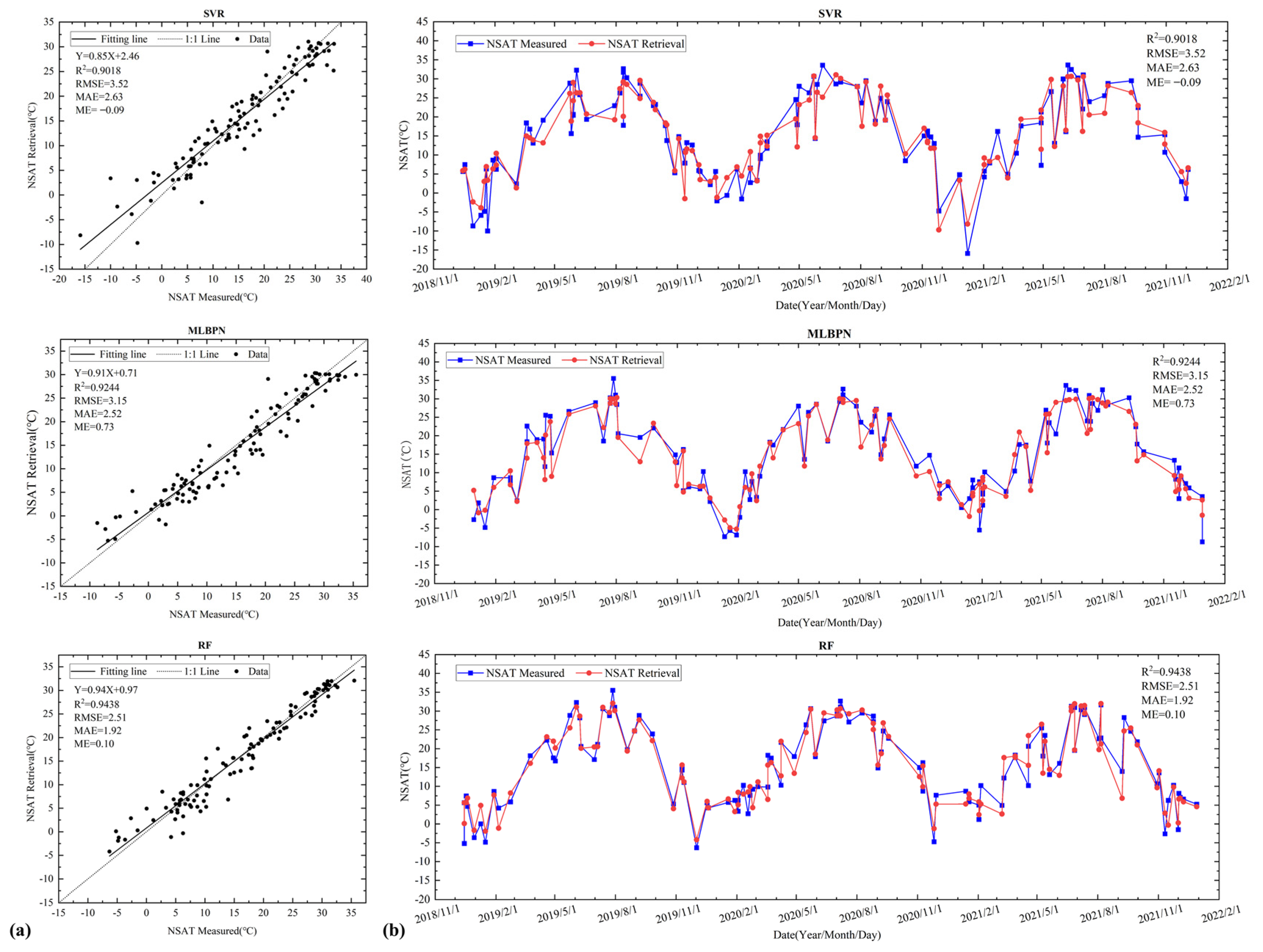
Figure 6 compares the measured NSATs from the ground observation stations with the retrieved values from Sentinel-2 data. The R2 of the regression line based on the RF model is larger than those based on the SVR and MLBPN models (see Figure 6a). Figure 6b randomly selected several samples (number = 112) captured from 2018 to 2021, where the RF-based model has higher NSAT retrieval accuracy with respect to all the four statistical indicators of R2, RMSE, MAE, and ME (see Table 2).
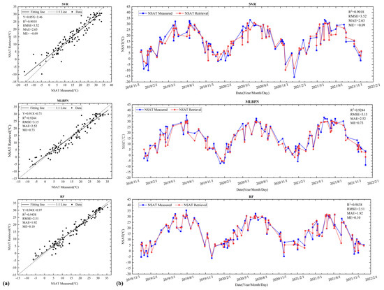
Figure 6.
Comparison between the measured and retrieved NSATs from Sentinel-2 data: (a) Scatterplots of the measured and retrieved values, where the solid line is the fitting line obtained by the line regression and the dashed line is the reference line of y = x. (b) Measured NSATs (blue line) versus retrieved NSATs (red lines) of the randomly selected samples from 2018–2021.
4.2. Validation Analysis
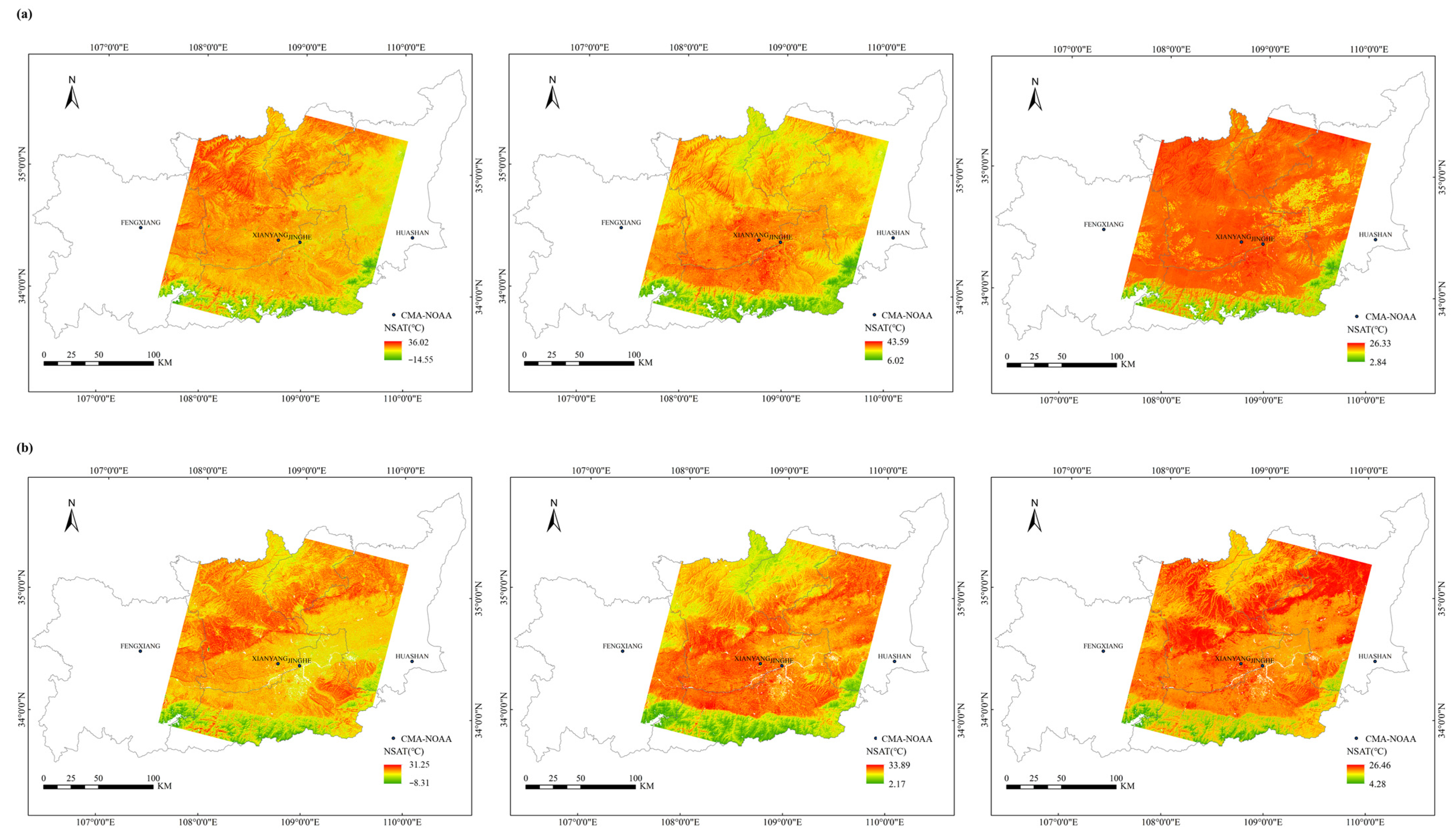
To further prove that the proposed RF-based model has the best performance, four study cases were randomly chosen for more precise qualitative analysis. Due to the influence of clouds, some data from the meteorological station FENGXIANG were deleted before each model was trained. Figure 7, Figure 8, Figure 9 and Figure 10 show the results of each model in the Guanzhong area using MODISTD data from 31 October 2018, MODISTN data from 28 August 2012, Landsat 8 data from 17 June 2016 and 7 April 2019, and Sentinel-2 data from 19 March 2020, respectively. At the same time, as illustrated in Table 3, Table 4, Table 5 and Table 6, the retrieval NSAT based on each model are also compared.

Figure 7.
Case study of MODISTD data in the Guanzhong area on 31 October 2018.

Figure 8.
Case study of MODISTN data in the Guanzhong area on 28 August 2012.
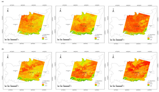
Figure 9.
Case study of Landsat 8 data in the Guanzhong area on (a) 17 June 2016 and (b) 7 April 2019.

Figure 10.
Case study of Sentinel-2 data in the Guanzhong area on 19 March 2020.

Table 3.
Comparison of the NSATs of four different monitoring stations on 31 October 2018.

Table 4.
Comparison of the NSATs of three different monitoring stations on 28 August 2012.

Table 5.
Comparison of the NSATs of two different monitoring stations on 17 June 2016 and 7 April 2019.

Table 6.
Comparison of the NSATs of four different monitoring stations on 19 March 2020.
In the case of MODISTD data, the RMSE of the SVR- and MLBPN-based models are 1.94 °C and 1.31 °C, the MAE are 1.88 °C and 1.21 °C, and the ME are −0.39 °C and −0.50 °C, respectively (see Table 7). When the measured NSATs are compared with the retrieved NSATs by the RF-based model, the RMSE is 1.20 °C, which is 0.74 °C smaller than the SVR model and 0.11 °C smaller than the MLBPN model. The MAE is 1.12 °C, which is 0.76 °C smaller than the SVR model and 0.09 °C smaller than the MLBPN model. The ME is −0.07 °C, which is 0.32 °C smaller than SVR and 0.43 °C smaller than MLBPN.

Table 7.
Comparison of the NSATs on 19 March 2020, respectively generated by the measurements, the SVR model, the MLBPN model, and the RF model and located at the positions of four different monitoring stations in the Guanzhong area.
In the case of MODISTN data, the RF-based model shows a significantly better performance than the SVR and MLBPN-based models. The RMSE of the SVR and MLBPN models on 28 August 2012 are 2.24 °C and 1.81 °C, the MAE are 2.07 °C and 1.73 °C, and the ME are 0.07 °C and −0.67 °C, respectively (see Table 7). The RMSE of the RF model is 0.56 °C, which is 1.68 °C smaller than the SVR model and 1.25 °C smaller than the MLBPN model. The MAE of the RF model is 0.54 °C, which is 1.53 °C smaller than the SVR model and 1.19 °C smaller than the MLBPN model. The ME of the RF model is 0.11 °C, which is 0.04 °C higher than the SVR model and 0.56 °C smaller than the MLBPN model.
In the case of Landsat 8 data, as illustrated in Table 7, the RMSE of the SVR and MLBPN models on 17 June 2016 and 7 April 2019 are 2.13 °C and 2.21 °C, the MAE are 1.40 °C and 1.55 °C, and the ME are −1.37 °C and −1.34 °C, respectively. The RMSE of the RF model is 1.43 °C, which is 0.70 °C smaller than the SVR model and 0.78 °C smaller than the MLBPN model. The MAE of the RF model is 1.15 °C, which is 0.25 °C smaller than the SVR model and 0.40 °C smaller than the MLBPN model. The ME of the RF model is 0.63 °C, which is 0.74 °C smaller than the SVR model and 0.71 °C smaller than the MLBPN model.
In the case of Sentinel-2 data, the RF-based model shows a significantly better performance than the SVR and MLBPN-based models. The RMSE of the SVR and MLBPN-based models on 19 March 2020 are 4.41 °C and 4.02 °C, the MAE are 3.32 °C and 3.22 °C, and the ME are 3.32 °C and 2.74 °C, respectively (see Table 7). The RMSE of the RF-based model is 1.71 °C, which is 2.70 °C smaller than SVR and 2.31 °C smaller than MLBPN. The MAE of the RF-based model is 1.59 °C, which is 1.73 °C smaller than SVR and 1.63 °C smaller than MLBPN. The ME of the RF model is 0.27 °C, which is 3.05 °C higher than SVR and 2.47 °C smaller than MLBPN. In addition, the retrieval results of Sentinel-2 with the SVR-based model shows some errors — the lowest NSAT is −40.92 °C. By comparing the relevant ground-truth NSAT data, it can be concluded that the accuracy and stability of the SVR-based model is not satisfactory.
Based on the analysis mentioned above, it is concluded that the RF-based model has the best performance with respect to both accuracy and stability. Meanwhile, the experiments employing the MODIS data revealed better NSAT retrieval results than the Landsat 8 and Sentinel-2 data.
5. Discussion
For further analysis, the residuals of the retrieval NSAT values have been calculated as well as compared in Figure 11.
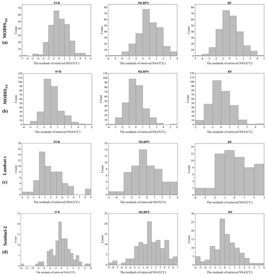
Figure 11.
Histograms of NSAT-retrieval residuals of the SVR, MLBPN and RF -based models.
Figure 11a shows the histograms of the NSAT-retrieval residuals, using the MODISTD data and based on different models. With the SVR-based model, there are 44.78%, 78.73%, and 94.40% of the residuals smaller than 1 °C, 2 °C and 3 °C respectively. With the MLBPN-based model, 49.25%, 80.60%, and 94.03% of the residuals are smaller than 1 °C, 2 °C, and 3 °C. With the RF model, the three proportions mentioned above have increased to 52.42%, 83.65%, and 95.17%, i.e. the RF-based model has revealed the best NSAT-retrieval performance in case of using the MODISTD data.
Figure 11b shows the histograms of NSAT-retrieval residuals using the MODISTN data. With the SVR-based model, there are 66.11%, 86.92%, and 96.65% residuals smaller than 1 °C, 2 °C, and 3 °C respectively. With the MLBPN-based model, 61.08%, 88.26%, and 98.32% of the residuals are smaller than 1 °C, 2 °C, and 3 °C. With the RF-based model, more residuals are located in the range of 0 °C ~ 3 °C − there are respectively 60.73%, 91.94%, and 98.99% of residuals in the range of 0 °C ~ 1 °C, 2 °C and 3 °C. Similar to the experiments using the MODISTD data, the RF model has revealed the best retrieval performance comparing to the SVR and MLBPN -based models.
Figure 11c shows the histograms of NSAT-retrieval residuals using the Landsat 8 data. With the SVR-based model, there are merely 35.09%, 54.38%, and 70.17% residuals smaller than 1 °C, 2 °C, and 3 °C respectively. With the MLBPN-based model, the corresponded proportions have increased to 40.35%, 70.18%, and 89.48%. With the RF-based model, the performance of the RF-based model becomes much better than the other two models, with more than 42.11%, 77.20% and 96.50% residuals located in the range of 0 °C~1 °C, 2 °C, and 3 °C.
Figure 11d shows the histograms of the retrieval residuals using the Sentinel-2 data and based on different models. With the SVR-based model, there are 30.63%, 53.15% and 64.84% of the residuals smaller than 1 °C, 2 °C, and 3 °C. With the MLBPN-based model, there are 27.93%, 47.75% and 66.67% of the residuals smaller than 1 °C, 2 °C and 3 °C. With the RF-based model, the residuals smaller than 1 °C, 2 °C and 3 °C increase to 40.18%, 59.83%, and 78.58%.
Based on the above analysis concerning on NSAT-retrieval residuals, it can be concluded that the RF-based model shows comprehensively better performance than the other two models.
Table 8 conducts further analysis of the NSAT retrieval residuals at different CMA-NOAA meteorological ground stations and in different seasons, produced by the RF-based model. With the MODISTD data, (a) the retrieval results in autumn are better than the other seasons and (b) the retrieval results at the XIANYANG meteorological ground station seem better than the other stations. With the MODISTN data, however, the spring becomes the ‘best’ season and the HUASHAN meteorological ground station become the ‘best’ station for the NSAT-retrievals. With the Landsat 8 data, the ‘best’ season goes back to autumn while the ‘best’ station changes to FENGXIANG. With the Sentinel-2 data, the retrieval results at JINGHE station/in winter have reached the highest accuracy. Thereby, it has not been found that there is a clear spatial or seasonal pattern concerning on the NSAT-retrieval residuals although the NSAT-retrieval performances of the RF-based model are very stable and satisfactory.

Table 8.
The analysis of retrieval residuals based on the RF model at different meteorological ground stations and in different seasons.
6. Conclusions
In this study, three machine-learning models based on SVR, MLBPN, and RF werte established to retrieve the NSAT from various multispectral satellite images in terms of MODIS daytime and nighttime data from 2010 to 2021, Landsat 8 data from 2013 to 2021, and Sentinel-2 data from 2018 to 2021. As well as the satellite images, the geospatial parameters, together with the time parameters, were also considered to enhance the accuracy of the NSAT retrieval.
The conducted experiments demonstrated that the RF-based model has better NSAT retrieval performance than the SVR- and MLBPN-based models with respect to both the accuracy and stability. With the MODISTD data, the RF-based model revealed a retrieval result with R2, RMSE, MAE, and ME equal to 0.9697, 1.48 °C, 1.17 °C, and 0.05 °C, respectively, where the RMSE and MAE are smaller than the NSAT retrieval model based on either SVR or MLBPN. With the MODISTN data, the RF-based model revealed a retrieval result with R2, RMSE, MAE, and ME equal to 0.9820, 1.21 °C, 0.95 °C, and −0.01 °C, respectively, where the R2 is larger and the RMSE, MAE, and ME are smaller than the SVR- and MLBPN-based models. With the Landsat 8 data, the RF-based model revealed a retrieval result with R2, RMSE, MAE, and ME equal to 0.9763, 1.54 °C, 1.27 °C, and 0.05 °C, respectively, where R2 is larger and the RMSE and MAE are smaller than the other two models. With the Sentinel-2 data, the NSAT result retrieved by the RF-based model has the largest R2 and the smallest RMSE and MAE. Moreover, several samples were randomly selected for more precise qualitative analysis, and the results also proved that the proposed RF-based model revealed the best NSAT retrieval performance.
Meanwhile, in the conducted experiments, as depicted in Table 2 and Table 7, the NSAT results retrieved from the MODIS data are generally better than those from Landsat 8 and Sentinel-2 data. Employing the MODISTN data, for instance, the R2 reaches 0.9820 and the RMSE and MAE are only slightly larger than 1.0 °C. In addition, it was also found that the RF model does not show significant pattern differences for the NSAT retrievals, which indicates that this model is stable and can thereby be widely utilized.
To sum up, the proposed RF-based model, together with the MODIS data, has the best NSAT retrieval results, which provides a reference for practical applications relevant to NSAT retrievals. Taking advantage of its high accuracy and stability, the RF-based model has the potential to be widely utilized in various applications concerning climate research and environmental studies. For example, the retrieved NSAT results can not only help to select the optimal location for the new meteorological ground stations to be constructed, but can also provide necessitated data for the correlation analysis between the NSAT and topographic changes, population distribution, land use, and climatic conditions, etc.
There are only four qualified CMA-NOAA stations located in the study area, which restricted the amount of sample data for model training and validation. In further research, the data from more CMA-NOAA stations could be involved to enhance the accuracy and/or the generic nature of the established NSAT retrieval models. In addition, although most of the clouds were removed through the quality control products in the data preprocessing, the remaining clouds still affected the retrieval accuracy. In the future, different algorithms need to be investigated to overcome the influence of clouds.
Author Contributions
Z.W. and M.Z. conceived and designed the study; Z.W. and M.Z. collected the data and completed the experiments; M.Z. initiated the overall research question and M.Z. found funding for this project; Z.W. drafted the paper; M.Z. critically read and revised the draft. All authors have read and agreed to the published version of the manuscript.
Funding
This work was funded in part by the Strategic Priority Research Program of the Chinese Academy of Sciences under Grant XDB40020200, and in part by the National Natural Science Foundation of China under Grant 41871315.
Institutional Review Board Statement
Not applicable.
Informed Consent Statement
Not applicable.
Data Availability Statement
Not applicable.
Acknowledgments
This research was supported by the Key Research and Development Program of Shaanxi Province (China) under Grant 2020SF-434. The data was supported by Data Center for Resources and Environmental Sciences, Chinese Academy of Sciences (RESDC) (http://www.resdc.cn, accessed on 15 August 2022).
Conflicts of Interest
The authors declare no conflict of interest.
References
- Rosenfeld, A.; Dorman, M.; Schwartz, J.; Novack, V.; Just, A.C.; Kloog, I. Estimating daily minimum, maximum, and mean near surface air temperature using hybrid satellite models across Israel. Environ. Res. 2017, 159, 297–312. [Google Scholar] [CrossRef] [PubMed]
- Leng, P.; Liao, Q.Y.; Ren, C.; Li, Z.L. A review of methods for estimating near-surface air temperature from remote sensing data. China Agric. Inform. 2019, 31, 1–10. (In Chinese) [Google Scholar]
- Bai, L.; Xu, Y.M.; He, M.; Li, N. Remote Sensing Inversion of Near Surface Air Temperature Based on Random Forest. J. Geo-Inf. Sci. 2017, 19, 390–397. (In Chinese) [Google Scholar]
- Zhu, S.Y.; Zhang, G.X. Progress in near surface air temperature retrieved by remote sensing technology. Adv. Earth Sci. 2011, 26, 724–730. (In Chinese) [Google Scholar]
- Yoo, C.; Im, J.; Park, S.; Quackenbush, L.J. Estimation of daily maximum and minimum air temperatures in urban landscapes using MODIS time series satellite data. ISPRS J. Photogramm. Remote Sens. 2018, 137, 149–162. [Google Scholar] [CrossRef]
- Basist, A.; Grody, N.C.; Peterson, T.C.; Williams, C.N. Using the Special Sensor Microwave/Imager to monitor land surface temperatures, wetness, and snow cover. J. Appl. Meteorol. 1998, 37, 888–911. [Google Scholar] [CrossRef]
- Gang, F.; Shen, Z.X.; Zhang, X.Z. Estimating air temperature of an alpine meadow on the Northern Tibetan Plateau using MODIS land surface temperature. Acta Ecol. Sin. 2011, 31, 8–13. [Google Scholar]
- Zhang, W.; Huang, Y.; Yu, Y.Q.; Sun, W.J. Empirical models for estimating daily maximum, minimum and mean air temperatures with MODIS land surface temperatures. Int. J. Remote Sens. 2011, 32, 9415–9440. [Google Scholar] [CrossRef]
- Cresswell, M.P.; Morse, A.P.; Thomson, M.C.; Connor, S.J. Estimating surface air temperatures, from Meteosat land surface temperatures, using an empirical solar zenith angle model. Int. J. Remote Sens. 1999, 20, 1125–1132. [Google Scholar] [CrossRef]
- Zhao, C.Y.; Nan, Z.R.; Cheng, G.D. Methods for modelling of temporal and spatial distribution of air temperature at landscape scale in the southern Qilian mountains, China. Ecol. Model. 2005, 189, 209–220. [Google Scholar]
- Xu, Y.M.; Liu, Y.H. Monitoring the Near-surface urban heat island in Beijing, China by satellite remote sensing. Geogr. Res. 2015, 53, 16–25. [Google Scholar] [CrossRef]
- Xu, Y.M.; Qin, Z.H.; Wan, H.X. Advances in the Study of Near Surface Air Temperature Retrieval from Thermal Infrared Remote Sensing. Remote Sens. Land Resour. 2011, 1, 9–14. (In Chinese) [Google Scholar]
- Prihodko, L.; Goward, S.N. Estimation of air temperature from remotely sensed surface observations. Remote Sens. Environ. 1997, 60, 335–346. [Google Scholar] [CrossRef]
- Nieto, H.; Sandholt, I.; Aguado, I.; Chuvieco, E.; Stisen, S. Air temperature estimation with MSG-SEVIRI data: Calibration and validation of the TVX algorithm for the Iberian Peninsula. Remote Sens. Environ. 2011, 115, 107–116. [Google Scholar] [CrossRef]
- Zhu, W.B.; Lv, A.F.; Jia, S.F. Estimation of daily maximum and minimum air temperature using MODIS land surface temperature products. Remote Sens. Environ. 2013, 130, 62–73. [Google Scholar] [CrossRef]
- Pape, R.; Löffler, J. Modelling spatio-temporal near-surface temperature variation in high mountain landscapes. Ecol. Model. 2004, 178, 483–501. [Google Scholar] [CrossRef]
- Hou, P.; Chen, Y.H.; Qiao, W.; Cao, G.Z.; Jiang, W.J.; Li, J. Near-surface air temperature retrieval from satellite images and influence by wetlands in urban region. Theor. Appl. Climatol. 2013, 111, 109–118. [Google Scholar] [CrossRef]
- Xu, Y.M.; Knudby, A.; Ho, H.C. Estimating daily maximum air temperature from MODIS in British Columbia, Canada. Int. J. Remote Sens. 2014, 35, 8108–8121. [Google Scholar] [CrossRef]
- Ho, H.C.; Knudby, A.; Sirovyak, P.; Xu, Y.M.; Hodul, M.; Henderson, S.B. Henderson. Mapping maximum urban air temperature on hot summer days. Remote Sens. Environ. 2014, 154, 38–45. [Google Scholar] [CrossRef]
- Emamifar, S.; Rahimikhoob, A.; Noroozi, A.A. Daily mean air temperature estimation from MODIS land surface temperature products based on M5 model tree. Int. J. Climatol. 2013, 33, 3174–3181. [Google Scholar] [CrossRef]
- Zhang, B.; Zhang, M.; Hong, D.F. Land surface temperature retrieval from Landsat 8 OLI/TIRS images based on back-propagation neural network. Indoor Built Environ. 2019, 30, 22–38. [Google Scholar] [CrossRef]
- Yu, Z.L.; Yang, X.J.; Shi, Y.Z. Evaluation of Urban Vulnerability to Drought in Guanzhong Area. Resour. Sci. 2012, 34, 581–588. (In Chinese) [Google Scholar]
- Dong, Y.X.; Wang, H.X.; Liu, H.J.; Zhao, R.X. Changing Trend and Sensitivity Analysis of Reference Crop Evapotranspiration in Guanzhong Region by Considering Climate Change. Water Sav. Irrig. 2019, 8, 113–119. (In Chinese) [Google Scholar]
- Fisthtahler, L. Standard data products from the MODIS science team. Geosci. Remote Sens. 1996, 2820, 230–244. [Google Scholar]
- Chu, Q.W.; Zhang, H.Q.; Wu, Y.W.; Feng, Z.K.; Chen, B. Application research of Landsat-8. Remote Sens. Inf. 2013, 28, 110–114. (In Chinese) [Google Scholar]
- Lin, R.C.; Chen, H.; Wei, Z.; Li, Y.N.; Zhang, B.Z.; Sun, H.R.; Cheng, M.H. Improved Surface Soil Moisture Estimation Model in Semi-Arid Regions Using the Vegetation Red-Edge Band Sensitive to Plant Growth. Atmosphere 2022, 13, 930. [Google Scholar] [CrossRef]
- Cheng, S.; Wang, Z. A Characteristics and Assessment Analysis of DEM Products. Prog. Geogr. 2005, 24, 99–108. (In Chinese) [Google Scholar]
- Vapnik, V.N. The Nature of Statistical Learning Theory; Springer: New York, NY, USA, 1995. [Google Scholar]
- Zhang, X.G. Introduction to statistical learning theory and support vector machines. Acta Autom. Sin. 2000, 26, 32–42. [Google Scholar]
- Zhou, Z.H. Machine Learning; Tsinghua University Press: Beijing, China, 2016; pp. 121–135. [Google Scholar]
- Kumar, M.P.; Sanjeev, K. Performance of back-propagation neural network in chaotic data time series forecasting and evaluation over parametric forecast: A case study for rainfall-runoff modelling over a river basin. Int. J. Inf. Technol. 2018, 10, 1–19. [Google Scholar]
- Tarvainen, T.; Vauhkonen, M.; Kolehmainen, V.; Arridge, S.R.; Kaipio, J.P. Coupled radiative transfer equation and diffusion approximation model for photon migration in turbid medium with low-scattering and non-scattering regions. Phys. Med. Biol. 2005, 50, 4913–4930. [Google Scholar] [CrossRef]
- Shen, T.W. Optimized Light Guide Plate Optical Brightness Parameter: Integrating Back-Propagation Neural Network (BPN) and Revised Genetic Algorithm (GA). Mater. Manuf. Process. 2014, 29, 1–8. [Google Scholar]
- Breiman, L. Random Forest. Mach. Learn. 2001, 45, 5–32. [Google Scholar] [CrossRef] [Green Version]
Publisher’s Note: MDPI stays neutral with regard to jurisdictional claims in published maps and institutional affiliations. |
© 2022 by the authors. Licensee MDPI, Basel, Switzerland. This article is an open access article distributed under the terms and conditions of the Creative Commons Attribution (CC BY) license (https://creativecommons.org/licenses/by/4.0/).

