Dimensionality Reduction by Similarity Distance-Based Hypergraph Embedding

Abstract

Dimensionality reduction (DR) is an essential pre-processing step for hyperspectral image processing and analysis. However, the complex relationship among several sample clusters, which reveals more intrinsic information about samples but cannot be reflected through a simple graph or Euclidean distance, is worth paying attention to. For this purpose, we propose a novel similarity distance-based hypergraph embedding method (SDHE) for hyperspectral images DR. Unlike conventional graph embedding-based methods that only consider the affinity between two samples, SDHE takes advantage of hypergraph embedding to describe the complex sample relationships in high order. Besides, we propose a novel similarity distance instead of Euclidean distance to measure the affinity between samples for the reason that the similarity distance not only discovers the complicated geometrical structure information but also makes use of the local distribution information. Finally, based on the similarity distance, SDHE aims to find the optimal projection that can preserve the local distribution information of sample sets in a low-dimensional subspace. The experimental results in three hyperspectral image data sets demonstrate that our SDHE acquires more efficient performance than other state-of-the-art DR methods, which improve by at least 2% on average.

1. Introduction

Hyperspectral remote sensing images have been taking a significant role in earth observation and climate models. Every collected pixel point indicates a high-dimensional sample that consists of a broad range of electromagnetic spectral band information [1,2]. Nevertheless, the high correspondence of adjacent bands not only leads to information redundancy but also requires tremendous time and space complexity, and the high-dimensional data also make hyperspectral image analysis a challenging task as a consequence of the Hughes phenomenon [3]. As Chang et al. proposed in [4], there can exist at most 94% redundant electromagnetic spectral band information, on the prem that adequate valuable information can be extracted for machine learning. In view of the aforementioned issues, hyperspectral data dimensionality reduction (DR) turns out to be a crucial part of data processing [5,6], usually via projecting original high-dimensional data into a low-dimensional space on the condition of maintaining as much valuable information as possible.

Supervised DR methods manage to increase the between-class separability and decrease the within-class divergency, such as linear discriminant analysis (LDA) [7], nonparametric weighted feature extraction (NWFE) [8], and local Fisher discriminant analysis (LFDA) [9]. LDA intends to maintain global discriminant information according to available labels, which is proven to work well in the case that samples from the same class follow Gaussian distribution. As an extension to LDA, LFDA is proposed to eliminate the limitation of LDA that requests the reduced dimensionality to be less than the total number of sample classes and ignores the local structural information.

However, in various practical applications, labeling samples exactly is labor intensive, computationally expensive, and time-consuming due to the limitations of experimental conditions, especially in hyperspectral remote sensing images [10]. So many research studies focus on unsupervised cases. Locality preserving projection (LPP) [11] and principal component analysis (PCA) are the representatives of unsupervised DR methods [12]. Different from LPP, on the purpose of preserving the local manifold structure of data, PCA aims at maintaining the global structure of data by maximizing sample variance.

A great deal of research demonstrates that high-dimensional data can be described by or similar to a smooth manifold in a low-dimensional space [13,14,15] and propose some DR methods based on manifold learning. Laplacian eigenmaps (LE) [14] try to maintain local manifold structure by constructing an undirected graph that indicates the pairwise relationship of samples. Locally linear embedding (LLE) [15] tries to reconstruct samples in a low-dimensional space while maintaining their local linear representation coefficients under the assumption that local samples follow a certain linear representation in a manifold patch. Yan et al. summarize relevant DR approaches and proposed a general graph embedding framework [16], which contains a series of variant graph embedding models, including neighborhood preserving embedding (NPE) [17], LPP, and several expanded versions to LPP [11,18,19]. For these graph embedding-based DR models, researchers usually utilize Euclidean distance to construct adjacent graphs [20], where vertices indicate samples and the weighted edges reflect pairwise affinities between two samples. Consequently, there exist two basic problems to be addressed.

• The conventional graph embedding-based DR methods, for example, LPP, aims to preserve the local adjacent relationship of samples by constructing a weight matrix which only takes the affinity between pairwise samples into account. However, the weight matrix fails to reflect the complex relationship of samples in high order [21], leading to the loss of information.
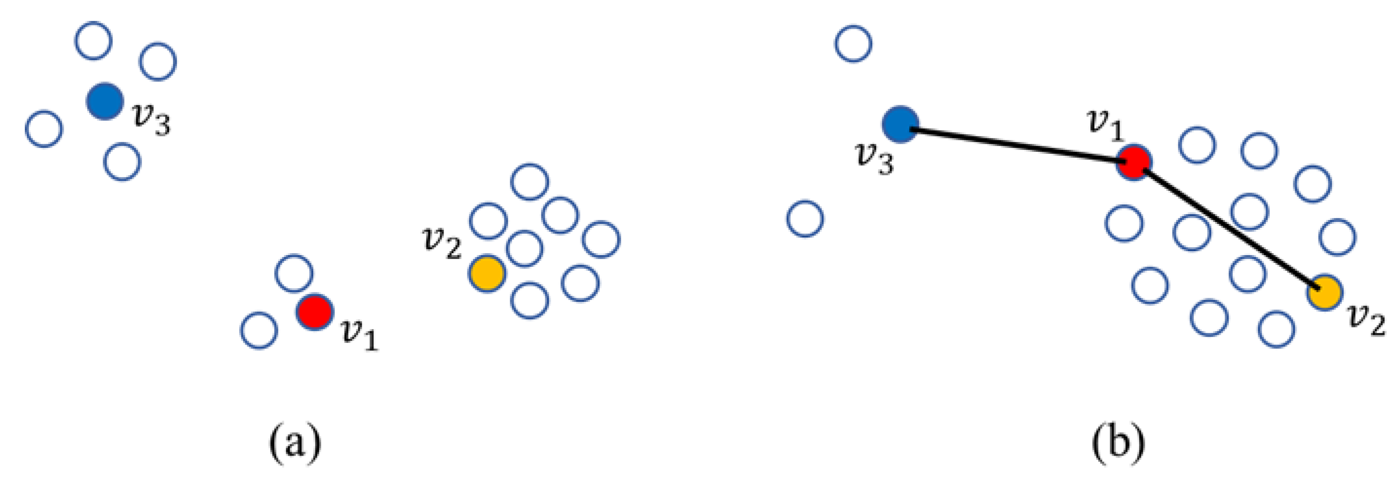
• When employed to calculate the similarity between two samples, the usual Euclidean distance is merely related to the two samples themselves but hardly considers the influence caused by their ambient samples [22,23] and ignores the distribution information of samples, which usually plays an important role for further data processing.

Accordingly, we propose a novel similarity distance-based hypergraph embedding method (SDHE) for unsupervised DR to solve the two above issues. Unlike conventional graph embedding-based models that only describe the affinity between two samples, SDHE is based on hypergraph embedding, which can take advantage of the complicated sample relationships in high order [24,25,26]. Besides, a novel similarity distance is defined instead of Euclidean distance to measure the affinity between samples because the similarity distance can not only discover complex geometrical structure information but also make use of the local distribution information of samples.

The remainder of our work is organized as follows. In Section 2, some related work is introduced, including the classic graph embedding model (LPP) and hypergraph embedding learning. Section 3 proposes our similarity distance-based hypergraph embedding method (SDHE) for dimensionality reduction in detail. In Section 4, we adopt three real hyperspectral images to evaluate the performance of SDHE in comparison with other related DR methods. Finally, Section 5 provides the conclusions.

2. Related Work

2.1. Notations of Unsupervised Dimensionality Reduction Problem

We focus on the unsupervised dimensionality reduction problem. The dataset is denoted as $V=\left[{\mathit{v}}_{\mathbf{1}},{\mathit{v}}_{\mathbf{2}},\dots ,{\mathit{v}}_{\mathit{n}}\right]\in R^{d\times n}$, where ${\mathit{v}}_{\mathit{i}}\in R^d$ represents the $i^{th}$ sample with $d$ feature values, $n$ denotes the number of total samples. In order to obtain a discriminative low-dimensional representation ${\mathit{y}}_{\mathit{i}}\in R^m (m<d)$ for each ${\mathit{v}}_{\mathit{i}}$, an optimal projection matrix $P\in R^{d\times m}$ is to be learned. We denote ${\mathit{y}}_{\mathit{i}}=P^T{\mathit{v}}_{\mathit{i}}$ or $Y=P^{T}V$, where $Y=\left[{\mathit{y}}_{\mathbf{1}},{\mathit{y}}_{\mathbf{2}},\dots ,{\mathit{y}}_{\mathit{n}}\right]\in R^{m\times n}$ as the data in the transformed space.

2.2. Locality Preserving Projection (LPP)

As is shown in [27], numerous high-dimensional observation data contain low-dimensional manifold structures, which motivates us to solve DR problems by extracting local metric information hidden in the low-dimensional manifold. Graph embedding has been proposed to present certain statistical or geometric characteristics of samples via constructing a graph embedding model [16]. In particular, LPP utilizes K nearest neighbors (KNN) algorithm to construct an adjacent graph so that local neighborhood structure is considered in feature space [17]. The basic derivation idea of the Formulas (1)–(4) comes from [17].

LPP is formulated to find a projection matrix $P\in R^{d\times m}$ by minimizing.

$$\begin{array}{c} \frac{1}{2}{\displaystyle {\displaystyle \sum }_{i,j=1}^n}{W}_{i,j}\Vert y_i-y_j\Vert {}_2^2\\ =\frac{1}{2}{\displaystyle {\displaystyle \sum }_{i,j=1}^n}{W}_{i,j}\Vert P^{\mathrm{T}}{\mathit{v}}_i-P^{\mathrm{T}}{\mathit{v}}_j\Vert {}_2^2\\ =trace\left(P^{\mathrm{T}}V\left(D-W\right)V^{\mathrm{T}}P\right)\\ =trace\left(P^{\mathrm{T}}VL{V}^{\mathrm{T}}P\right)\\ \end{array}$$

(1)

where $D$ is a diagonal matrix with diagonal entries $D_{i,i}={\displaystyle \sum }_{j=1}^n{W}_{i,j}$, and $\mathrm{L}=D-W$ is Laplacian matrix. The symmetric weighted matrix $\mathrm{W}$ is defined on an adjacent graph, in which each entry $W_{i,j}$ corresponds to a weighted edge denoting the similarity between two samples. The most popular approach to define $W_{i,j}$ is as below:

$$W_{i,j}=\{\begin{array}{cc}\exp \left(-\Vert {\mathit{v}}_{\mathit{i}}-{\mathit{v}}_{\mathit{j}}\Vert {}_2^2/t\right)\hfill & {\mathit{v}}_{\mathit{i}} \mathrm{and} {\mathit{v}}_{\mathit{j}} \mathrm{are} \mathrm{neighbors} \hfill \\ 0\hfill & \mathrm{otherwise}\hfill \end{array}$$

(2)

where $t$ denotes the heat kernel parameter, and $W_{i,j}$ increases monotonously with the decrease of distance between ${\mathit{v}}_{\mathit{i}}$ and ${\mathit{v}}_{\mathit{j}}$.

Therefore, if samples ${\mathit{v}}_{\mathit{i}}$ and ${\mathit{v}}_{\mathit{j}}$ are the K nearest neighbors of each other, the mapped samples ${\mathbf{y}}_{\mathbf{i}}$ and ${\mathbf{y}}_{\mathbf{j}}$ are close to each other in the transformed space as well, due to the heavy penalty incurred by $W_{i,j}$. Usually a constraint $P^{T}VD{V}^{T}P=I$ is imposed to ensure a meaningful solution, where $I$ denotes the identity matrix. Then the final optimization problem can be written as follows:

$$\begin{gathered} \mathrm{m}\underset{\mathbf{P}}{\mathrm{in}} \mathit{trace}\left(P^{\mathrm{T}}{\mathrm{VLV}}^{\mathrm{T}}P\right) \\ \mathrm{s}.\mathrm{t}. P^{\mathrm{T}}VD{V}^{\mathrm{T}}P=I \end{gathered}$$

(3)

The solution to the optimal projection matrix can be translated into the following generalized eigenvalues problem.

$$VL{V}^{\mathrm{T}}P=VD{V}^{\mathrm{T}}P\Lambda$$

(4)

where $P$ denotes the eigenvector matrix of ${\left(VD{V}^T\right)}^{-1}VL{V}^T$ and $\Lambda$ denotes the eigenvalue matrix whose diagonal entries are eigenvalues corresponding with $P$.

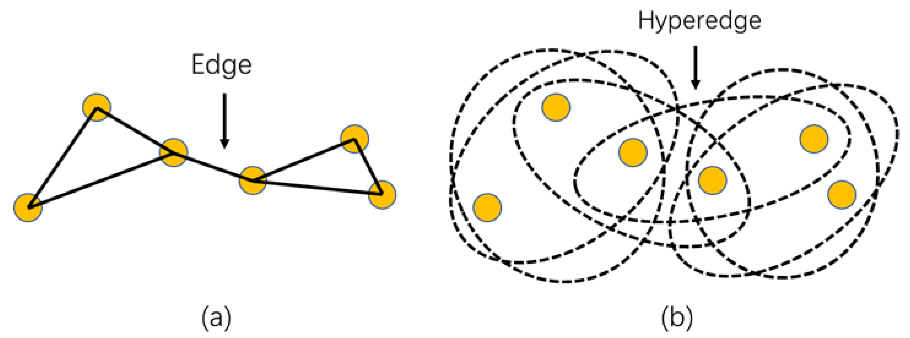
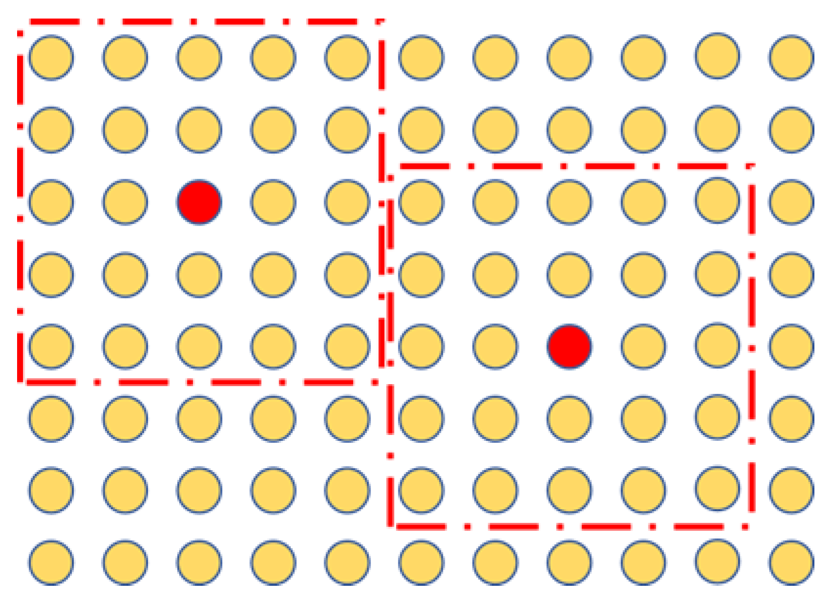
2.3. Hypergraph Embedding

Since hypergraph theory is proposed, hypergraph learning has made promising progress in many applications in recent years, and the basic derivation idea of the Formulas (5)–(8) comes from [26,28,29]. As an extension to the classic graph, a hypergraph facilitates the representation of a data structure by capturing adjacent sample relationships in high order, which overcomes the limitation of a classic graph in that each edge only considers the affinity between pairwise samples. Unlike a classic graph, where a weighted edge links up two vertices, the hyperedge consists of several nodes in a certain neighborhood. Figure 1 is taken as an example of a classic graph and hypergraph.

The hypergraph $\mathit{G}=\left(V,E,w\right) \mathrm{is} \mathrm{constructed} \mathrm{as} \mathrm{the} \mathrm{following}$. Here, $V=\left[{\mathit{v}}_{\mathbf{1}},{\mathit{v}}_{\mathbf{2}},\dots ,{\mathit{v}}_{\mathit{n}}\right]\in R^{d\times n}$ denotes the vertex set corresponding to samples, and $E=\left[{\mathit{E}}_{\mathbf{1}},{\mathit{E}}_{\mathbf{2}},\dots ,{\mathit{E}}_{\mathit{n}}\right]$ denotes the hyperedge set, in which each hyperedge is assigned a positive weight $w\left(E_i\right)$. For a certain vertex, its K nearest neighbors (let K = 2 in Figure 1b) are found out to make up a hyperedge, and an incidence matrix $H\in R^{n\times n}$ is defined to express the affiliation between vertices and hyperedges as follows:

$$H_{i,j}=h\left({\mathit{v}}_i,{\mathit{E}}_{\mathit{j}}\right)=\{\begin{array}{cc}1\hfill & \mathrm{if}{\mathit{v}}_{\mathit{i}}\in {\mathit{E}}_{\mathit{j}}\hfill \\ 0\hfill & \mathrm{otherwise}\hfill \end{array}$$

(5)

Then each hyperedge is assigned with a weight computed by:

$$w_i=w\left({\mathit{E}}_i\right)={\displaystyle \sum }_{v_j\in E_i}\exp \left(-\Vert {\mathit{v}}_j-{\mathit{v}}_i\Vert {}_2^2/h\right)$$

(6)

where $h$ is the Gaussian kernel parameter. According to incidence matrix $H$ and hyperedge weight $w\left(E\right)$, the vertex degree for each vertex ${\mathit{v}}_{\mathit{i}}\in V$ is defined as:

$$d_i=d\left(v_i\right)={\displaystyle \sum }_{j=1}^n{w}_j{H}_{i,j}$$

(7)

and the hyperedge degree ${\delta }_i$ for each hyperedge ${\mathit{E}}_{\mathit{i}}\in E$ is defined as:

$${\delta }_i=\delta \left({\mathit{E}}_i\right)={\displaystyle \sum }_{j=1}^n{H}_{j,i}$$

(8)

Namely, ${\delta }_i$ denotes the number of vertices that belong to the same hyperedge ${\mathit{E}}_{\mathit{i}}$.

3. Proposed Method

In this section, we propose a novel unsupervised DR method called similarity distance-based hypergraph embedding (SDHE). Below we first give a kind of hypergraph embedding-based similarity, then construct a novel similarity distance, and finally, propose a similarity distance-based hypergraph embedding model for DR.

3.1. Hypergraph Embedding-Based Similarity

It is a reasonable choice to describe a high-order similarity relationship with a hypergraph rather than a simple graph. Because the hypergraph has the characteristic that each hyperedge connects more than two vertices and these vertices share one weighted hyperedge, i.e., the samples in the same hyperedge are regarded as a whole. A hyperedge $E_i$ consists of the sample $v_i$ together with its K nearest neighbors, thus an incidence matrix $H\in R^{n\times n}$ is defined by Equation (5) to represent the affiliation between vertices and hyperedges. Then a positive weight $w_i$ is assigned to the hyperedge $E_i$ according to Equation (6), and the weight of hyperedge ${\mathit{E}}_{\mathit{i}}$ is calculated by summing up the certain relationships between sample ${\mathit{v}}_{\mathit{i}}$ with its $K$ nearest neighbors.

However, the weight of hyperedge excessively relies on parameter $K$. If $K$ is too small, the hypergraph will approach a simple graph inducing that the hypergraph cannot depict high order sample relationship sufficiently. Otherwise, if $K$ is too large, one hyperedge would connect too much number of vertices sharing the common weight of the hyperedge, which fails to reflect vertices’ own unique similarity characteristics. It is worth noting that outliers also share hyperedge weight with other vertices, and stated thus, hypergraph embedding is sensitive to outliers (usually noise), so we manage to modify the disadvantage by constructing a robust similarity to alleviate the sensitiveness of outliers. The similarity $s_{i,j}$ between arbitrary two samples ${\mathit{v}}_{\mathit{i}}$ and ${\mathit{v}}_{\mathit{j}}$ is defined as follows:

$$\begin{array}{cc}\hfill s_{i,j}& ={\displaystyle {\displaystyle \sum }_{{\mathit{E}}_k\in E}}{\displaystyle {\displaystyle \sum }_{v_i,{\mathit{v}}_j\in V}}w\left({\mathit{E}}_k\right)h\left({\mathit{v}}_i,{\mathit{E}}_k\right)h\left({\mathit{v}}_j,{\mathit{E}}_k\right)\hfill \\ \hfill & ={\displaystyle {\displaystyle \sum }_{k,i,j=1}^n}{w}_k{H}_{i,k}{H}_{j,k}\hfill \end{array}$$

(9)

where the notations $H$ and $w$ have been defined in Equations (5) and (6), respectively.

According to Equation (9), the similarity between samples ${\mathit{v}}_{\mathit{i}}$ and ${\mathit{v}}_{\mathit{j}}$ is calculated by summing up all the weight of these common hyperedges they both belong to. The weight of common hyperedge is associated with local sample distribution; next, we explains how it works. On the one hand, each hyperedge connects $K+1$ vertices so that the weight $w_i$ of hyperedge ${\mathit{E}}_{\mathit{i}}$ becomes larger if these $K+1$ vertices are distributed compactly, and vice versa. If an outlier and its $K$ nearest neighbors make up a hyperedge, then the hyperedge has a smaller weight because the distribution of these vertices is more scattered. In other words, outlier has little contribution to the weight of hyperedge, making the measure of similarity more robust. On the other hand, each vertex can belong to several different hyperedges. When two vertices are very close to each other, they can participate in more of the same hyperedges and have a higher similarity as we expect. Considering the sample distribution means we can mine more valuable information from the training samples of the same size according to their local structure and distribution relationship in the hypergraph, especially small-size samples. Our experiments conducted on different data sets have confirmed the conclusion, as shown in Section 4.

3.2. Similarity Distance Construction

Euclidean distance is the most popular tool to measure the similarity between samples in graph embedding-based DR methods [30]. However, it is not very accurate for analyzing hyperspectral images problem. For example, as depicted in Figure 2a, three samples ${\mathit{v}}_{\mathbf{1}},{\mathit{v}}_{\mathbf{2}}$ and ${\mathit{v}}_{\mathbf{3}}$ are from three different classes respectively, and ${\mathit{v}}_{\mathbf{1}}$ is closer to ${\mathit{v}}_{\mathbf{2}}$ but far away from ${\mathit{v}}_{\mathbf{3}}$ in Euclidean Distance. Accordingly, ${\mathit{v}}_{\mathbf{1}}$ and ${\mathit{v}}_{\mathbf{2}}$ are more likely to be misclassified into the same class when we ignore some complex structure and distribution information, which probably leads to the increase of classification error. For another example, as depicted in Figure 2b, Euclidean distance from ${\mathit{v}}_{\mathbf{1}}$ to ${\mathit{v}}_{\mathbf{2}}$ is equivalent to that from ${\mathit{v}}_{\mathbf{1}}$ to ${\mathit{v}}_{\mathbf{3}}$. But ${\mathit{v}}_{\mathbf{1}}$ and ${\mathit{v}}_{\mathbf{2}}$ are more likely to belong to the same class according to the distribution of samples, which cannot be reflected intuitively by Euclidean distance. So we are motivated to propose a novel similarity distance to replace Euclidean distance.

It is natural that if two samples have high similarity, they are likely to come from the same class, even though we know nothing about their exact labels in unsupervised DR problem. That is to say, when two similar samples are mapped to low-dimensional space, they ought to be close to each other according to their similarity in original feature space. Directly using the similarity to represent the distance relationship encounters the problem of non-uniform measurement, so we normalize the similarity by defining the relative similarity $r_{i,j},$ as below:

$$r_{i,j}=\frac{S_{i,j}-S_{min}}{S_{max}-S_{min}}$$

(10)

where $s_{i,j}$ has been defined in Equation (9), $s_{min}$ and $s_{max}$ denote the minimum and maximum elements in similarity matrix $S$, respectively. Thus $s_{i,j}=s_{max}$ corresponds to $r_{i,j}=1$ and $s_{i,j}=s_{min}=0$ corresponds to $r_{i,j}=0$. As a normalized metric of $s_{i,j}$, $r_{i,j}$ reflects the probability that samples $i$ and $j$ belong to the same class. Besides, the relative similarity matrix consisting of entries $r_{i,j}$ is sparse because the majority of entries $r_{i,j}=s_{i,j}=0$, i.e., there exists no hyperedge that contains samples $i$ and $j$ simultaneously.

Based on the relative similarity $r_{i,j}$, a novel similarity distance $E{D}_{i,j}$ is defined for measuring the location relationship of samples as below:

$$E{D}_{i,j}=1-\log \left(r_{i,j}\right)$$

(11)

where $0<r_{ij}\le 1$ and $E{D}_{i,j}\ge 1$. Specially, if $r_{ij}=0$, we define $E{D}_{i,j}=+\infty$. And the similarity distance is symmetric, i.e., $E{D}_{i,j}=E{D}_{j,i}$.

In order to get an intuitive recognition of similarity distance, Figure 2b gives a directed diagram to explain how it works. Despite the equivalent Euclidean distance from ${\mathit{v}}_{\mathbf{1}}$ to ${\mathit{v}}_{\mathbf{2}}$ or ${\mathit{v}}_{\mathbf{3}}$, the sample distribution around ${\mathit{v}}_{\mathbf{1}}$ and ${\mathit{v}}_{\mathbf{2}}$ is denser than that around ${\mathit{v}}_{\mathbf{1}}$ and ${\mathit{v}}_{\mathbf{3}}$. According to Equation (6), denser distribution leads to the larger weight of hyperedge and corresponds to larger similarity. A larger similarity means smaller similarity distance, which demonstrates that the similarity distance between ${\mathit{v}}_{\mathbf{1}}$ and ${\mathit{v}}_{\mathbf{2}}$ is smaller than that between ${\mathit{v}}_{\mathbf{1}}$ and ${\mathit{v}}_{\mathbf{3}}$. Obviously, the result accords with our intuitive judgment.

One advantage of Euclidean distance is simple and easy to acquire, but also limits the amount of information it can take along with. Whereas the geometrical structure of hyperspectral data in high-dimensional feature space is complex and hard to learn, Euclidean distance cannot effectively reflect the interaction between samples. However, via using similarity distance, we can discover crucial information that is not directly exhibited through geometrical distance and make great progress in analyzing hyperspectral images DR problem.

3.3. Similarity Distance-Based Hypergraph Embedding Model

As portrayed in the above two sections, we extract similarity from hypergraph embedding, then utilize the similarity to construct similarity distance. Now we propose our similarity distance-based hypergraph embedding (SDHE) model for DR, whose basic idea is to find out a projection matrix $P$ that projects original high-dimensional data to low-dimensional manifold space while preserving the similarity distance among samples.

Similar to LPP, a penalty factor $E{W}_{i,j}$ is defined to balance the similarity distance between samples $i$ and $j$ in transformed space as follows:

$$E{W}_{i,j}=\exp \left(-E{D}_{i,j}^2/t\right)$$

(12)

where $E{D}_{i,j}$ is formulated in Equation (11) and $t$ is a positive heat kernel parameter. Thus, the optimization problem of SDHE is formulated to minimize.

$$\begin{array}{c} \frac{1}{2}{\displaystyle {\displaystyle \sum }_{i,j=1}^n}{EW}_{i,j}\Vert {\mathbf{P}}^{\mathrm{T}}{\mathit{v}}_i-{\mathbf{P}}^{\mathrm{T}}{\mathit{v}}_j{\Vert }_2^2\\ =\frac{1}{2}{\displaystyle {\displaystyle \sum }_{i,j=1}^n}({\mathbf{P}}^{\mathrm{T}}{\mathit{v}}_i){}^{\mathrm{T}}{EW}_{i,j}{\mathbf{P}}^{\mathrm{T}}{\mathit{v}}_i+\frac{1}{2}{\displaystyle {\displaystyle \sum }_{i,j=1}^n}({\mathbf{P}}^{\mathrm{T}}{\mathit{v}}_j){}^{\mathrm{T}}{EW}_{i,j}{\mathbf{P}}^{\mathrm{T}}{\mathit{v}}_j-{\displaystyle {\displaystyle \sum }_{i,j=1}^n}({\mathbf{P}}^{\mathrm{T}}{\mathit{v}}_i){}^{\mathrm{T}}{EW}_{i,j}{\mathbf{P}}^{\mathrm{T}}{\mathit{v}}_j\\ ={\displaystyle {\displaystyle \sum }_{i=1}^n}({\mathbf{P}}^{\mathrm{T}}{\mathit{v}}_i){}^{\mathrm{T}}{D}_{i,i}{\mathbf{P}}^{\mathrm{T}}{\mathit{v}}_i-{\displaystyle {\displaystyle \sum }_{i,j=1}^n}({\mathbf{P}}^{\mathrm{T}}{\mathit{v}}_i){}^{\mathrm{T}}{EW}_{i,j}{\mathbf{P}}^{\mathrm{T}}{\mathit{v}}_j\\ =\mathit{trace}\left({\mathbf{P}}^{\mathrm{T}}{\mathbf{VDV}}^{\mathrm{T}}\mathbf{P}\right)-\mathit{trace}\left({\mathbf{P}}^{\mathrm{T}}{\mathbf{V}\left(\mathbf{EW}\right)\mathbf{V}}^{\mathrm{T}}\mathbf{P}\right)\\ =\mathit{trace}\left({\mathbf{P}}^{\mathrm{T}}\mathbf{V}\right(\mathbf{D}-\mathbf{EW}\left){\mathbf{V}}^{\mathrm{T}}\mathbf{P}\right)\\ =\mathit{trace}\left({\mathbf{P}}^{\mathrm{T}}{\mathbf{VLV}}^{\mathrm{T}}\mathbf{P}\right)\end{array}$$

(13)

where $D$ is a diagonal matrix with diagonal entries $D_{i,i}={\displaystyle \sum }_{j=1}^{n}E{W}_{i,j}$, and $L=D-EW$ is the Laplacian matrix.

Therefore, if samples ${\mathit{v}}_{\mathit{i}}$ and ${\mathit{v}}_{\mathit{j}}$ have a small similarity distance in the original feature space, the mapped samples ${\mathit{y}}_{\mathit{i}}$ and ${\mathit{y}}_{\mathit{j}}$ would be close to each other in the transformed feature space as well due to the heavy penalty incurred by $E{W}_{i,j}$. In order to avoid a degeneracy solution, the final optimization problem is formulated as follows by adding a regularization term.

$$\underset{P}{\max }\frac{trace\left(P^{\mathrm{T}}VD{V}^{\mathrm{T}}P\right)}{trace\left(P^{\mathrm{T}}VL{V}^{\mathrm{T}}P\right)}$$

(14)

which is a trace-ratio problem, can be reduced to solve the following generalized eigenvalues problem.

$$VD{V}^{\mathrm{T}}P=\mathsf{\lambda }VL{V}^{\mathrm{T}}P$$

(15)

where $\mathsf{\lambda }$ represents generalized eigenvalue. The optimal projection matrix $P=\left[{\mathit{P}}_{\mathbf{1}},{\mathit{P}}_{\mathbf{2}},\dots ,{\mathit{P}}_{\mathit{m}}\right]$ is acquired by choosing eigenvectors corresponding with the first $m$ maximum eigenvalues.

An outline of SDHE Algorithm 1 is summarized as follows:

Algorithm 1: SDHE

Require: Training samples $V=\left[{\mathit{v}}_{\mathbf{1}},{\mathit{v}}_{\mathbf{2}},\dots ,{\mathit{v}}_{\mathit{n}}\right]\in R^{d\times n}$, dimensionality of transformed space $m$, the number of nearest neighbors K, the Gaussian kernel parameters h and t

Ensure:  The optimal projection matrix $P^{*}\in R^{d\times m}$.

Step 1: Embed hypergraph by using K nearest neighbors algorithm and get affiliation relationship $H_{i,j}$ according to Equation (5); Step 2: Calculate the weight of each hyperedge $w_i$ according to Equation (6); Step 3: Calculate the similarity $s_{i,j}$ by           $s_{i,j}={\displaystyle \sum _{k,i,j=1}^n}{W}_k{H}_{i,k}{H}_{j,k};$ Step 4: Translate the similarity $s_{i,j}$ into relative similarity $r_{ij}$:            $s_{min}=min\left(s_{i,j}\right) ;$           $s_{max}=max\left(s_{i,j}\right) ;$            $r_{i,j}=\frac{s_{i,j}-s_{min}}{s_{max}-s_{min}};$ Step 5: Construct the similarity distance by $E{D}_{i,j}=1-\log \left(r_{i,j}\right)$; Step 6: Construct penalty factor by $E{W}_{i,j}=\exp \left(-E{D}_{i,j}^2/t\right)$; Step 7: Calculate $D$ and $L$; Step 8: Solve generalized eigenvalues problem $VD{V}^{T}P=\mathsf{\lambda }VL{V}^{T}P;$ Step 9: $P^{*}=\left[{\mathit{P}}_{\mathbf{1}},{\mathit{P}}_{\mathbf{2}},\dots ,{\mathit{P}}_{\mathit{m}}\right]$ is the eigenvectors corresponded with $m$ maximum eigenvalues.

4. Result and Discussion

In this section, the validity of our proposed SDHE method was tested on three hyperspectral data sets compared with some related DR methods. The DR effectiveness was evaluated according to classification accuracy, which was calculated by the nearest neighbor (NN) classifier after different DR methods were conducted on the data set, respectively.

4.1. Hyperspectral Images Data Set

Our experiments were conducted by employing three standard hyperspectral image data sets as follows; more details are shown in Section 4.3.

4.1.1. Pavia University

The Pavia University scene was gathered by the reflective optics system imaging spectrometer (ROSIS) optical sensor over Pavia, northern Italy. It is a 610 × 610 pixels image that was divided into 9 classes grounds truth with 103 spectral bands after some invalid samples had to be removed.

4.1.2. Salinas

The Salinas scene was acquired by the airborne visible/infrared imaging spectrometer (AVIRIS) sensor over Salinas Valley, Southern California, in 1998. This area consists of 512 × 217 pixels with 224 spectral bands. Discarded 20 water absorption bands, it contains 16 classes of observations with 204 spectral bands.

4.1.3. Kennedy Space Center

The Kennedy Space Center (KSC) data was acquired by the Airborne Visible/Infrared Imaging Spectrometer (AVIRIS) instrument over the KSC, Florida, in 1996. It consists of 13 classes of observations with 176 spectral bands after we discarded uncalibrated and noisy bands that cover the region of water absorption features.

4.2. Experimental Setup

4.2.1. Training Set and Testing Set

Considering the distinct scale and distribution of the data sets above, we randomly choose 15, 20 or 25 samples from per class in Pavia University, Salinas and KSC scenes to make up the training sets, respectively. Naturally, the rest of the samples were regarded as testing sets. In addition, a random 10-fold validation method was adopted, that is, the partition process was repeated 10 times independently to weaken the influence of random bias.

4.2.2. Data Pre-Processing

As Camps-Valls G et al. proposed in [31], we utilized spatial mean filtering to enhance hyperspectral data classification. For example, assuming a pixel ${\mathit{x}}_{\mathit{i}}$ with coordinate $\left(p_i,q_i\right)$, we denote its local pixel neighborhood $N\left(x_i\right),$ as below:

$$N\left(x_i\right)=\left\{x\left(p,q\right)\mid p\in \left[p_i-a,p_i+a\right],q\in \left[q_i-a,q_i+a\right]\right\},a=0,1,2,\dots$$

(16)

For pixels at the edge of image, the samples were mirrored before using spatial mean filtering. Then all the pixels had their spatial neighborhood $N\left(x\right)$ including ${\left(2a+1\right)}^2$ pixels, where $2a+1$ indicates the width of spatial filtering window. Finally, each pixel $\mathit{x}$ is represented by:

$$\widehat{x}=\frac{1}{{(2a+1)}^2}{\displaystyle \sum }_{s=1}^{{(2a+1)}^2}{x}_s$$

(17)

In our experiments, we set $a=2$ for all the hyperspectral images, that is, the width of spatial neighborhood is 5, as depicted in Figure 3. Besides, the filtered data is normalized by min-max scaling as a popular routine.

4.2.3. Comparison and Evaluation

In order to evaluate the effectiveness of different DR methods, the testing set is transformed into low-dimensional data utilizing the optimal projection matrix, which is learned from the training set. As a contract, two classical unsupervised DR methods PCA [12] and LPP [11], two state-of-the-art unsupervised DR methods BH and SH [32], as well as two supervised DR methods LFDA [9] and NWFE [8], were compared with our proposed SDHE method. As a baseline to illustrate others, the raw data (RAW) is also directly classified without DR. In our experiments, the nearest neighbor (NN) classifier is adopted for classification, and we can acquire overall accuracy (OA), average accuracy (AA), and kappa coefficient (KC) together with their standard deviations (STD) to evaluate these DR methods.

4.2.4. Parameter Selection

It is essential to select the appropriate parameters for different DR methods in our experiments. The number of nearest neighbors $K$ is selected from the given set of $\left\{3,5,7,9,11\right\}$, the Gaussian kernel parameters h and $t$ are selected from the given set of $\left\{2^{-8},2^{-7},\cdots ,2^7,2^8\right\}$, respectively. In order to decrease the influence of random bias, we repeat each single experiment 10 times, with every combination of parameters and randomly divided training and testing sets. The optimal combination of parameters is acquired associated with the highest mean overall accuracy (OA).

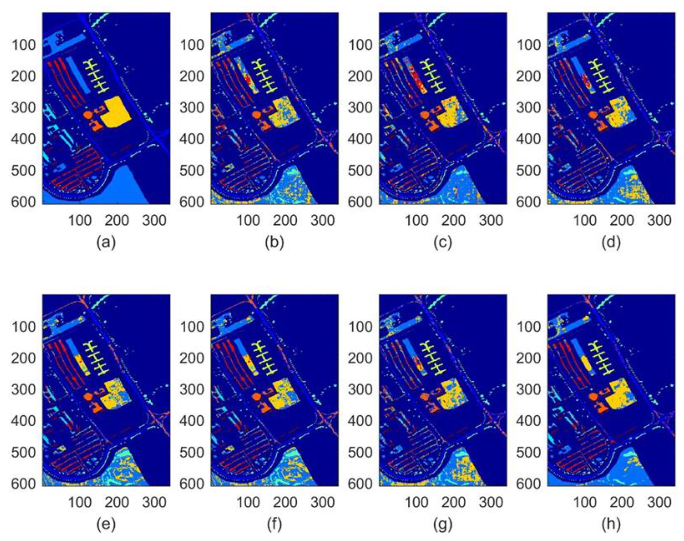
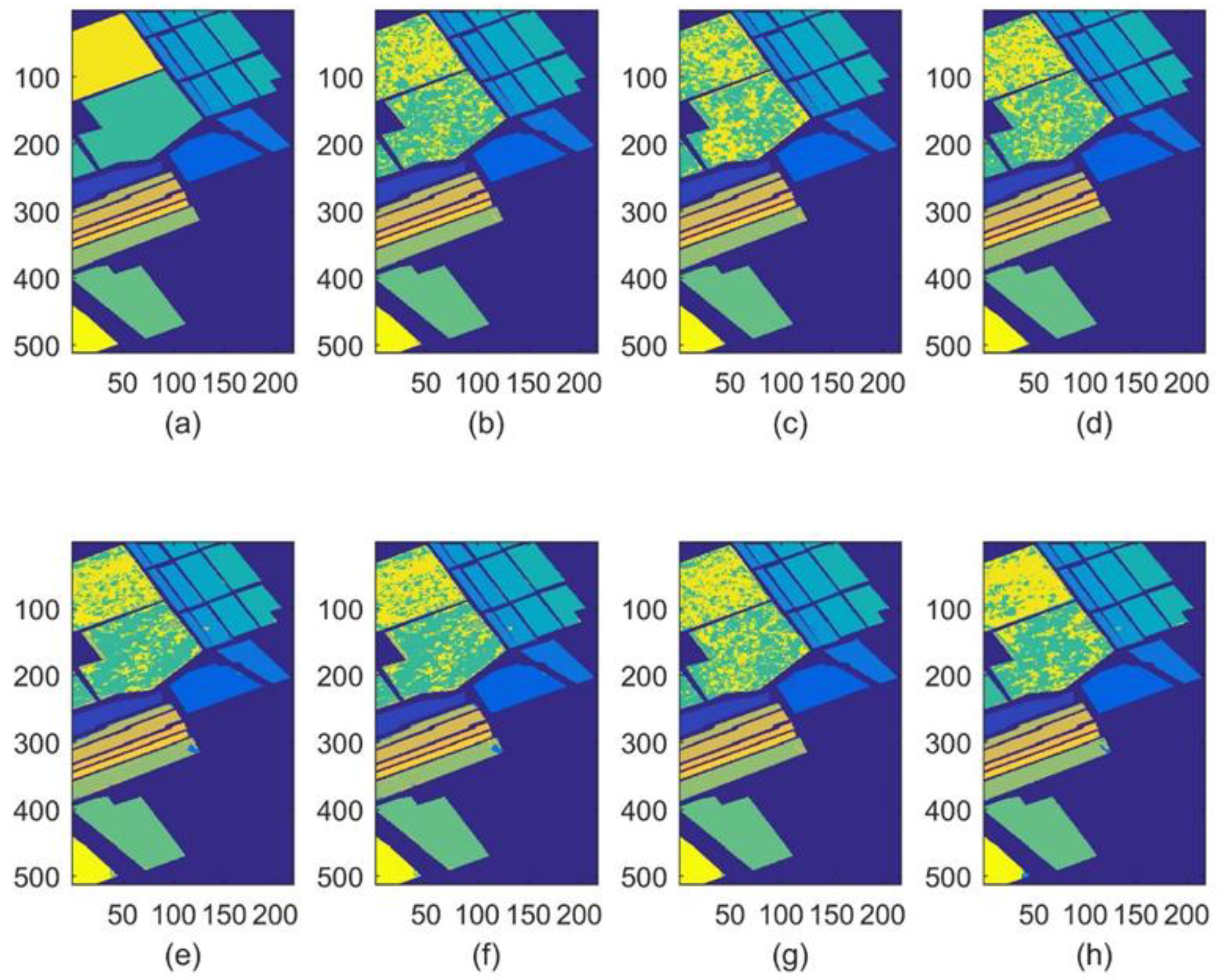
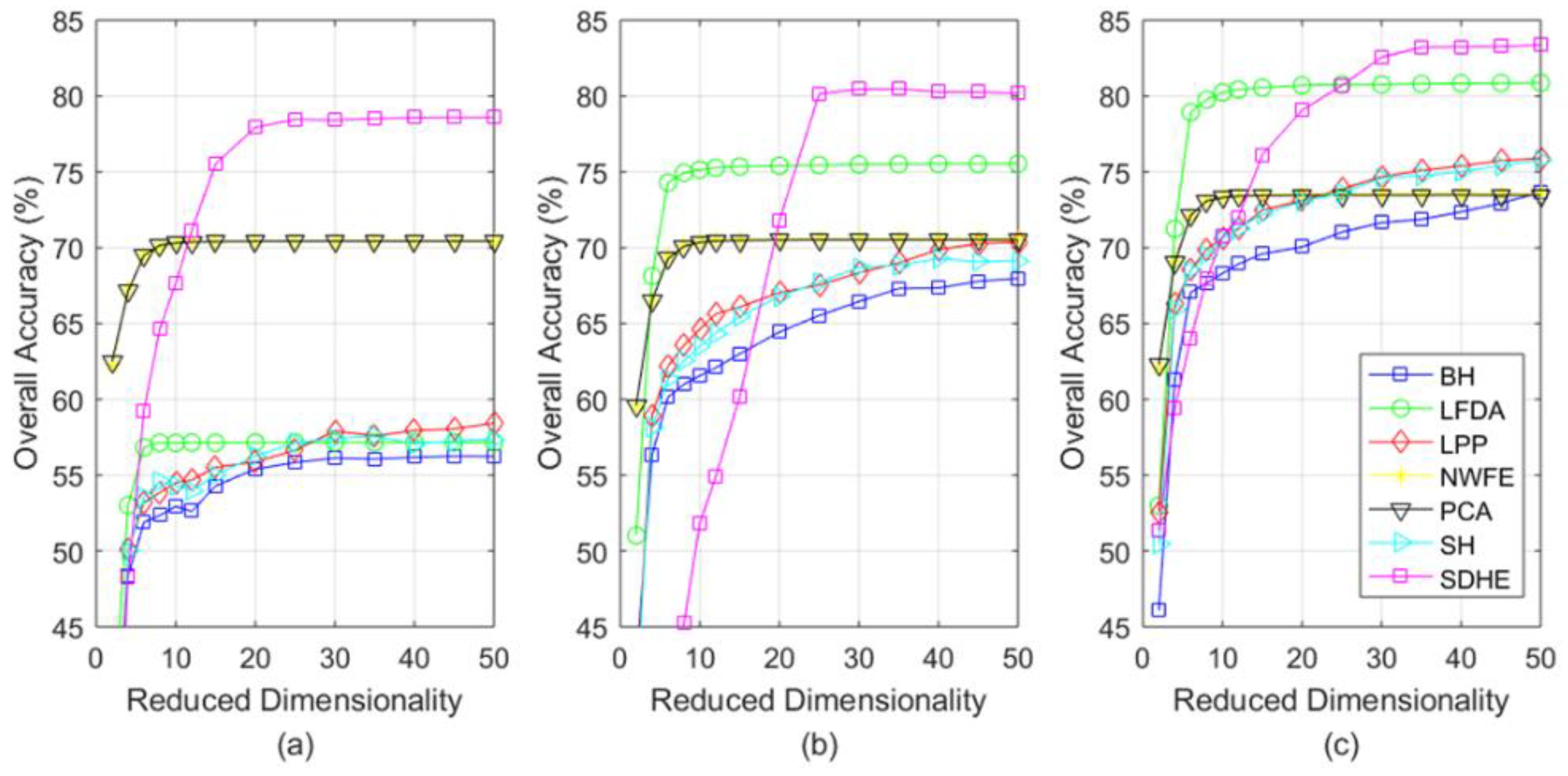
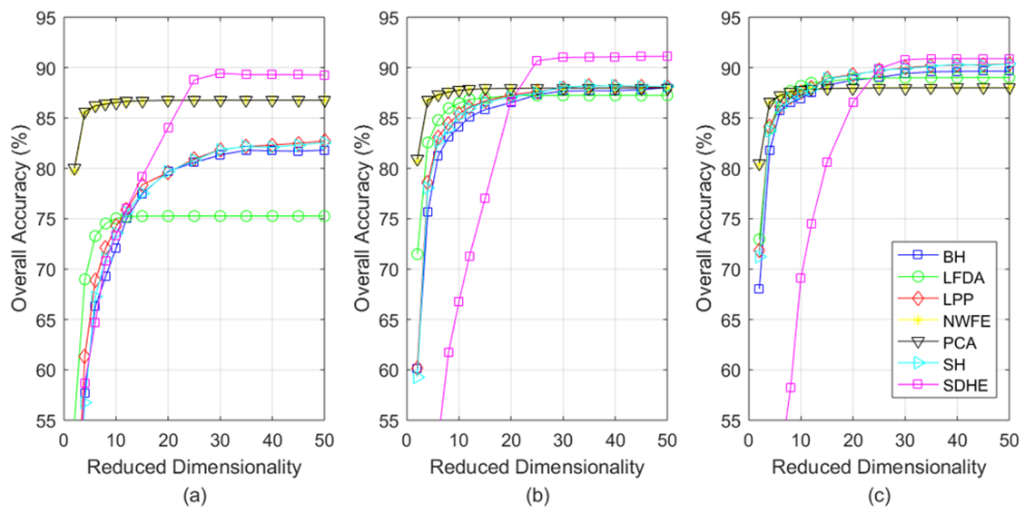
4.3. Experimental Results

To have a further knowledge of our data sets,

Table 1. Ground truth classes and their individual samples number for Pavia University.

Number	Class	Samples
1	Asphalt	6631
2	Meadows	18,649
3	Gravel	2099
4	Trees	3064
5	Painted metal sheets	1345
6	Bare Soil	5029
7	Bitumen	1330
8	Self-Blocking Bricks	3682
9	Shadows	947
Total		42,776

,

Table 2. Ground truth classes and their individual samples number for Salinas.

Number	Class	Samples
1	Brocoil-green-weeds-1	2009
2	Brocoil-green-weeds-2	3726
3	Fallow	1976
4	Fallow-rough-plow	1394
5	Fallow-smooth	2678
6	Stubble	3959
7	Celery	3579
8	Grapes-untrained	11,271
9	Soil-vinyard-develop	6203
10	Corn-senesced-green-weeds	3278
11	Lettuce-romaine-4wk	1068
12	Lettuce-romaine-5wk	1927
13	Lettuce-romaine-6wk	916
14	Lettuce-romaine-7wk	1070
15	Vinyard-untrained	7268
16	Vinyard-vertical-trellis	1807
Total		54,129

and

Table 3. Ground truth classes and their individual samples number for KSC.

Number	Class	Samples
1	Scrub	761
2	Willow swamp	243
3	CP hammock	256
4	CP/Oak hammock	252
5	Slash pine	161
6	Oak/Broadleaf hammock	229
7	Hardwood swamp	105
8	Graminoid marsh	431
9	Spartina marsh	520
10	Cattail marsh	404
11	Salt marsh	419
12	Mud flats	503
13	Water	927
Total		5211

present the detailed ground truth classes and the number of their individual samples for Pavia University, Salinas, and KSC respectively.

First, we randomly choose 20 samples per class to comprise the training set, and the rest samples are regarded as a testing set. Then we can learn a projection matrix with the training set and conduct DR on the testing set by making use of the projection matrix learned before. The reduced dimensionality is fixed at 30, which turns out to be a relatively stable state for all the related DR methods in our experiments. Finally, the nearest neighbor (NN) classifier is adopted for classification, and these processes are repeated 10 times to get the mean classification accuracy with the corresponding standard deviation. Below we display our experimental results in the form of a Table and Figure together with some relevant discussion.

The experimental results for the three hyperspectral data sets are displayed in

Table 4. Classification accuracy (%) at 30-dimensionality for Pavia University with the training set of 20 samples per class.

Class	RAW	BH	LFDA	LPP	NWFE	PCA	SH	SDHE
1	67.82 ± 5.17	61.51 ± 5.88	70.34 ± 6.08	56.46 ± 6.69	67.99 ± 5.15	67.84 ± 5.16	57.88 ± 5.01	73.68 ± 8.17
2	63.54 ± 5.55	60.97 ± 5.78	75.98 ± 4.01	69.00 ± 8.34	63.56 ± 5.52	63.54 ± 5.55	69.40 ± 8.23	79.54 ± 5.75
3	62.37 ± 5.10	53.46 ± 6.34	65.97 ± 6.19	50.26 ± 5.25	62.46 ± 5.17	62.34 ± 5.13	48.84 ± 5.79	69.74 ± 6.78
4	86.70 ± 3.13	84.76 ± 4.87	89.01 ± 4.86	89.14 ± 3.28	86.76 ± 3.11	86.70 ± 3.13	89.08 ± 3.94	87.53 ± 6.02
5	99.52 ± 0.36	100.00 ± 0	99.92 ± 0.11	100.00 ± 0	99.52 ± 0.36	99.52 ± 0.36	100.00 ± 0	99.77 ± 0.40
6	75.52 ± 6.47	72.68 ± 4.49	74.53 ± 8.99	74.13 ± 4.98	75.58 ± 6.47	75.52 ± 6.47	73.33 ± 5.36	86.70 ± 3.70
7	80.05 ± 3.58	81.23 ± 5.15	84.25 ± 7.46	66.92 ± 9.20	79.98 ± 3.66	80.02 ± 3.57	67.10 ± 4.81	88.93 ± 5.30
8	74.10 ± 5.79	61.16 ± 5.08	59.92 ± 6.00	52.92 ± 5.70	74.22 ± 5.84	74.09 ± 5.79	54.36 ± 5.37	74.18 ± 8.81
9	99.08 ± 0.46	99.15 ± 0.44	98.79 ± 0.71	98.91 ± 0.70	99.09 ± 0.47	99.08 ± 0.46	98.88 ± 0.80	99.26 ± 0.35
OA	70.52 ± 2.77	66.45 ± 2.48	75.49 ± 2.21	68.35 ± 3.53	70.58 ± 2.77	70.52 ± 2.77	68.71 ± 3.07	80.45 ± 3.68
AA	78.74 ± 1.40	74.99 ± 1.22	79.86 ± 1.28	73.08 ± 1.85	78.80 ± 1.42	78.74 ± 1.40	73.21 ± 1.61	84.37 ± 2.96
KC	60.88 ± 3.68	55.48 ± 3.29	67.48 ± 2.94	58.00 ± 4.69	60.96 ± 3.68	60.87 ± 3.68	58.47 ± 4.08	74.06 ± 4.88

,

Table 5. Classification accuracy (%) at 30-dimensionality for Salinas with the training set of 20 samples per class.

Class	RAW	BH	LFDA	LPP	NWFE	PCA	SH	SDHE
1	98.49 ± 0.59	99.79 ± 0.43	98.93 ± 1.51	99.43 ± 0.60	98.49 ± 0.59	98.49 ± 0.59	99.61 ± 0.38	99.50 ± 0.76
2	99.61 ± 0.46	99.88 ± 0.24	99.78 ± 0.50	99.09 ± 1.61	99.62 ± 0.46	99.61 ± 0.46	99.59 ± 0.63	99.90 ± 0.16
3	97.07 ± 1.70	98.56 ± 1.41	98.30 ± 1.28	99.36 ± 0.99	97.11 ± 1.67	97.06 ± 1.70	99.18 ± 0.81	99.16 ± 1.55
4	97.90 ± 1.60	98.53 ± 1.43	98.15 ± 0.64	99.02 ± 0.58	97.93 ± 1.57	97.89 ± 1.62	98.96 ± 0.61	98.52 ± 0.91
5	93.92 ± 1.26	96.58 ± 0.87	93.67 ± 2.02	96.86 ± 0.92	93.91 ± 1.28	93.92 ± 1.27	96.90 ± 0.85	95.64 ± 1.79
6	99.55 ± 0.55	99.84 ± 0.43	99.74 ± 0.54	99.97 ± 0.07	99.55 ± 0.55	99.55 ± 0.55	99.96 ± 0.07	99.77 ± 0.43
7	98.76 ± 0.54	99.47 ± 0.55	99.64 ± 0.37	99.70 ± 0.20	98.76 ± 0.55	98.76 ± 0.54	99.68 ± 0.21	99.54 ± 0.30
8	68.68 ± 3.58	62.60 ± 5.21	67.41 ± 5.72	65.74 ± 5.01	68.64 ± 3.54	68.64 ± 3.59	65.45 ± 5.33	75.46 ± 4.40
9	98.70 ± 0.55	99.87 ± 0.20	98.80 ± 2.19	99.54 ± 1.30	98.71 ± 0.54	98.70 ± 0.55	99.78 ± 0.56	99.80 ± 0.22
10	86.22 ± 4.13	94.67 ± 1.89	92.28 ± 2.52	95.28 ± 1.88	86.27 ± 4.14	86.22 ± 4.13	95.43 ± 1.69	92.38 ± 1.77
11	95.29 ± 2.19	98.46 ± 1.17	98.44 ± 1.26	98.94 ± 0.83	95.33 ± 2.20	95.29 ± 2.19	98.89 ± 0.72	98.38 ± 1.41
12	99.94 ± 0.08	99.51 ± 0.51	98.22 ± 1.83	99.63 ± 0.44	99.95 ± 0.08	99.94 ± 0.08	99.27 ± 1.48	99.44 ± 1.51
13	98.67 ± 1.78	99.01 ± 1.33	98.95 ± 0.87	99.23 ± 0.91	98.65 ± 1.77	98.67 ± 1.78	99.11 ± 1.13	99.74 ± 0.44
14	95.70 ± 2.87	97.00 ± 1.77	97.15 ± 2.28	96.86 ± 2.38	95.71 ± 2.85	95.70 ± 2.87	96.84 ± 2.44	97.88 ± 1.88
15	73.89 ± 4.75	72.64 ± 5.66	65.79 ± 6.05	69.82 ± 5.47	73.80 ± 4.83	73.87 ± 4.75	70.47 ± 6.15	78.80 ± 3.70
16	96.56 ± 1.82	98.82 ± 0.58	98.63 ± 0.44	99.13 ± 0.37	96.56 ± 1.82	96.55 ± 1.82	99.17 ± 0.33	98.04 ± 0.73
OA	87.98 ± 0.76	87.67 ± 0.74	87.24 ± 1.53	87.99 ± 0.79	87.97 ± 0.75	87.97 ± 0.76	88.07 ± 0.78	91.01 ± 1.37
AA	93.68 ± 0.35	94.70 ± 0.22	93.99 ± 0.85	94.85 ± 0.32	93.69 ± 0.35	93.68 ± 0.35	94.89 ± 0.33	95.75 ± 0.59
KC	86.61 ± 0.85	86.27 ± 0.83	85.79 ± 1.71	86.62 ± 0.88	86.59 ± 0.84	86.59 ± 0.85	86.71 ± 0.87	89.98 ± 1.53

and

Table 6. Classification accuracy (%) at 30-dimensionality for KSC with the training set of 20 samples per class.

Class	RAW	BH	LFDA	LPP	NWFE	PCA	SH	SDHE
1	94.55 ± 3.90	90.20 ± 6.86	86.13 ± 7.04	92.47 ± 3.33	94.55 ± 3.90	94.55 ± 3.90	92.46 ± 4.31	95.03 ± 2.75
2	90.45 ± 4.25	89.78 ± 4.99	89.06 ± 5.86	91.75 ± 4.59	90.49 ± 4.25	90.45 ± 4.25	91.84 ± 5.23	94.39 ± 3.84
3	92.63 ± 1.60	88.18 ± 7.74	86.86 ± 6.80	86.44 ± 5.88	92.63 ± 1.62	92.58 ± 1.61	86.10 ± 9.55	95.89 ± 3.22
4	61.51 ± 5.50	54.05 ± 6.12	72.76 ± 8.26	43.97 ± 7.92	61.72 ± 5.64	61.42 ± 5.53	51.98 ± 6.95	81.64 ± 4.18
5	72.84 ± 4.93	74.47 ± 7.36	90.00 ± 6.43	68.01 ± 7.00	72.70 ± 4.98	72.70 ± 5.04	71.28 ± 11.8	94.04 ± 3.89
6	80.86 ± 2.85	84.74 ± 6.36	90.38 ± 7.89	83.11 ± 6.25	80.86 ± 2.85	80.81 ± 2.87	82.49 ± 5.68	94.59 ± 3.30
7	99.18 ± 1.83	97.29 ± 4.50	96.82 ± 5.98	97.65 ± 3.11	99.18 ± 1.83	99.18 ± 1.83	97.65 ± 2.68	99.53 ± 0.94
8	88.44 ± 3.88	85.23 ± 8.67	90.24 ± 3.39	91.05 ± 6.76	88.44 ± 3.88	88.44 ± 3.88	89.81 ± 6.01	96.45 ± 3.02
9	96.20 ± 2.13	95.14 ± 3.29	93.60 ± 4.68	96.82 ± 2.86	96.20 ± 2.13	96.18 ± 2.16	96.66 ± 3.34	99.92 ± 0.13
10	93.54 ± 4.47	94.48 ± 2.39	92.60 ± 2.17	95.10 ± 2.66	93.72 ± 4.51	93.52 ± 4.44	95.78 ± 2.07	99.14 ± 1.22
11	98.97 ± 1.29	99.22 ± 0.77	97.72 ± 2.85	99.25 ± 0.68	98.97 ± 1.29	98.97 ± 1.29	99.10 ± 1.08	99.17 ± 1.43
12	92.88 ± 4.37	80.70 ± 6.26	79.36 ± 5.98	84.16 ± 7.35	93.21 ± 4.36	92.88 ± 4.37	83.35 ± 6.64	94.95 ± 2.92
13	100.00 ± 0	98.64 ± 0.82	98.69 ± 0.85	97.76 ± 2.48	100.00 ± 0	100.00 ± 0	98.24 ± 0.77	99.99 ± 0.03
OA	92.38 ± 1.18	89.60 ± 2.43	90.32 ± 2.07	90.11 ± 1.76	92.44 ± 1.14	92.37 ± 1.17	90.46 ± 1.83	96.61 ± 0.78
AA	89.39 ± 1.08	87.09 ± 2.34	89.56 ± 1.79	86.73 ± 1.66	89.44 ± 1.05	89.36 ± 1.07	87.44 ± 1.92	95.75 ± 0.74
KC	91.49 ± 1.32	88.39 ± 2.72	89.19 ± 2.31	88.95 ± 1.96	91.55 ± 1.28	91.47 ± 1.31	89.35 ± 2.05	96.22 ± 0.87

, and the bolded experimental values indicate the best performance among all the competitive DR methods. In addition, the optimal parameters for our SDHE are $K=5,h=32, t=0.0313$ for Pavia University, $K=5, h=16, t=0.0313$ for Salinas, $K=3,h=0.0156,t=0.1250$ for KSC.

As listed in Table 4, Table 5 and Table 6, our proposed SDHE acquires prominently higher classification accuracy than other competitive DR methods in AA, OA, and KC. Note that both BH and SH belong to hypergraph embedding DR methods, as well as our SDHE, but they have a comparatively poor performance in that they ignore the sample distribution information and Euclidean distance cannot reveal intrinsic similarity. What is more, the results of RAW, NWFE, and PCA are very similar to each other, which demonstrates that the transformed feature spaces founded by NWFE or PCA cannot promote classification effectiveness but reduce the redundancy of high-dimensional data to make data processing more efficient, but they still outperform other DR methods for KSC. All the competitive DR methods except for SDHE reach a very near classification accuracy for Salinas.

For each individual class, the SDHE also prevailed over the other related DR methods in the total 6 of 9 classes for Pavia University, 5 of 16 classes for Salinas and 11 of 13 classes for KSC. Remarkably, the SDHE was notably superior to others, especially in the classes that had a comparatively lower classification accuracy, especially the 1st, 2nd and 3rd classes in Pavia University, the 8th and 15th classes in Salinas and the 4th, 5th and 6th classes in KSC. Although the SDHE was inferior to the others in several classes, the classification accuracy gaps between these classes of different DR methods were narrow.

In order to present the classification effectiveness of different DR methods intuitively, the samples of testing set were given different pseudo labels, which were simulated by NN classifier after we conducted corresponding DR methods. Then, the results are portrayed via classification maps in Figure 4, Figure 5 and Figure 6. For each Figure, the subfigure (a) indicates the ground truth of original hyperspectral data set, the subfigure (b–h) indicates the performance of BH, LFDA, LPP, NWFE, PCA, SH and our proposed SDHE, respectively. The higher classification accuracy means the less miscellaneous samples in the corresponding subfigure, and the key points were highlighted by a white circle in subfigure (h) of Figure 4 and Figure 5. Obviously, there are less miscellaneous samples in our proposed SDHE in contrast to the others.

To research the DR effectiveness on the different sizes of training sets, we randomly selected 15, 20, or 25 samples per class as the training set, and the rest samples were regarded as the testing set, respectively. Then the related experimental results, including OA (%) and STD for the three hyperspectral data sets are listed in

Table 7. Classification accuracy (%) at 30-dimensionality for the different sizes of training sets in Pavia University.

Method	The Size of Training Set
	15	20	25
RAW	70.43 ± 1.75	70.52 ± 2.77	73.47 ± 1.18
BH	56.14 ± 1.72	66.45 ± 2.48	71.65 ± 3.09
LFDA	57.16 ± 8.41	75.49 ± 2.21	80.76 ± 1.25
LPP	57.92 ± 2.57	68.35 ± 3.54	74.68 ± 2.51
NWFE	70.46 ± 1.75	70.58 ± 2.77	73.56 ± 1.18
PCA	70.42 ± 1.75	70.52 ± 2.77	73.47 ± 1.18
SH	57.43 ± 1.94	68.71 ± 3.08	74.60 ± 2.94
SDHE	78.41 ± 5.13	80.45 ± 3.67	82.56 ± 2.87

,

Table 8. Classification accuracy (%) at 30-dimensionality for the different sizes of training sets in Salinas>.

Method	The Size of Training Set
	15	20	25
RAW	86.77 ± 1.83	87.98 ± 0.76	88.00 ± 0.92
BH	81.32 ± 1.29	87.67 ± 0.74	89.40 ± 0.76
LFDA	75.27 ± 3.32	87.24 ± 1.53	88.99 ± 0.98
LPP	81.87 ± 1.05	87.99 ± 0.79	89.97 ± 1.11
NWFE	86.78 ± 1.85	87.97 ± 0.75	88.00 ± 0.92
PCA	86.76 ± 1.83	87.97 ± 0.76	87.98 ± 0.92
SH	81.86 ± 1.57	88.07 ± 0.78	89.90 ± 1.24
SDHE	89.43 ± 1.07	91.01 ± 1.37	90.78 ± 0.87

and

Table 9. Classification accuracy (%) at 30-dimensionality for the different sizes of training sets in KSC>.

Method	The Size of Training Set
	15	20	25
RAW	91.16 ± 0.58	92.38 ± 1.18	93.39 ± 0.57
BH	73.23 ± 2.35	89.60 ± 2.43	93.99 ± 0.61
LFDA	60.05 ± 11.54	90.32 ± 2.07	94.56 ± 1.03
LPP	74.05 ± 2.88	90.11 ± 1.76	93.91 ± 0.92
NWFE	91.11 ± 0.58	92.44 ± 1.14	93.38 ± 0.56
PCA	91.15 ± 0.58	92.37 ± 1.17	93.38 ± 0.58
SH	73.73 ± 1.80	90.46 ± 1.83	94.53 ± 0.70
SDHE	95.88 ± 1.04	96.61 ± 0.92	97.49 ± 0.44

.

Besides considering the influence of reduced dimensionality on classification accuracy, Figure 7, Figure 8 and Figure 9 draw relevant curve figures according to the same training sets with their OAs of different DR methods listed in Table 7, Table 8 and Table 9. By adding the x-axis to denote the change of reduced dimensionality, the performances of different DR methods are depicted in Figure 7, Figure 8 and Figure 9. For each Figure, the subfigure (a–c) indicates the training set of 15, 20, or 25 samples per class, respectively.

According to Table 7, Table 8 and Table 9, despite the size of training sets ranging from 15 to 25 samples per class, the SDHE always performs best among all the related DR methods. We found that the smaller size of the training set, the greater superiority our SDHE had than other DR methods. Note that when the training set consisted of 15 samples per class, the LFDA not only performed poorly in OA but also had a much higher STD, which means the performance of LFDA was sensitive to the small size training set because the local within-class scatter matrix was likely to be singular or ill-conditioned. But the LFDA had a rapid increase in classification accuracy with the increasing size of the training set. However, as listed in Table 8, the mean OA decreases with the size of the training set became larger, from 20 to 25 samples per class for Salinas, because of the parameter values were discrete, which limits the optimal accuracy the model can achieve. Thus, it is a normal phenomenon.

According to Figure 7, Figure 8 and Figure 9, the SDHE still outperforms other DR methods in the different sizes of training sets. With the increase of reduced dimensionality, the classification accuracy increases rapidly in the beginning but then reaches a steady level, which proves the reasonability of analyzing the results at 30-dimensionality previously. It is worth mentioning that the smaller size of the training set the more outstanding advantage our SDHE possesses, for the reason that the use of hypergraph and similarity distance help to mine more hidden information. Empirically, when the reduced dimensionality is more than 15, our SDHE shows a remarkable advantage.

5. Conclusions

Three main contributions of our work are listed as follows:

• A novel similarity distance is proposed via hypergraph construction. Compared with Euclidean distance; it can make better use of the sample structure and distribution information; for the reason that it considers not only the adjacent relationship between samples but also the mutual affinity of samples in high order.
• The proposed similarity distance is employed to optimize DR problem, i.e., our proposed SDHE aims to maintain the similarity distance in a low-dimensional space. In this way, the similarity in capturing the structure and distribution information between samples is inherited in the transformed space.
• When applied for the classification task of three different hyperspectral images, our SDHE is proved to perform more effectively, especially the size of the training set is comparatively small. As shown in Table 7, Table 8 and Table 9, our method improves OA, AA, and KC by at least 2% on average on different data sets.

Furthermore, our work is to use a graph to mine the intrinsic geometric information of the data. Graph data itself is a kind of structured data that is different from our work. For graph learning, there are many ways to perform dimensionality reduction in graphs, such as weight pruning, vertex pruning, and joint weight and vertex pruning [33]. In addition, compared with graphs, where each sample is a structure, the input of our data is a vector. If the input is tensor, tensor decompositions will be suitable [34]. Compared with the neural network [35], which often requires large-scale computation, our method is more like a single-layer neural network with a special objective function, which has the advantage of effectively utilizing lightweight computing resources.

We propose a similarity distance-based hypergraph embedding method (SDHE) for unsupervised dimensionality reduction. First, the hypergraph embedding technique is employed to discover the complicated affinity of samples in high order. Then we take advantage of the complicated affiliation between vertices and hyperedges to construct a similarity matrix, which includes the local distribution information of samples. Finally, based on hypergraph embedding and the similarity matrix, a novel similarity distance is proposed to be an alternative substitute for Euclidean distance, which can better reflect complicated geometry structure information of data well. The experimental results in three hyperspectral image data sets demonstrate that our proposed SDHE obtains more efficient performance than other popular DR methods. For further study, we prepare to derive the similarity distance to semi-supervised model learning, which can combine discriminative analysis with structure and distribution information, and wish to make good progress in the remote sensing field of a climate model.

References

1. Tan, K.; Wang, X.; Zhu, J.; Hu, J.; Li, J. A novel active learning approach for the classification of hyperspectral imagery using quasi-Newton multinomial logistic regression. Int. J. Remote Sens. 2018, 39, 3029–3054. [Google Scholar] [CrossRef]
2. Zhong, Z.; Li, J.; Luo, Z.; Chapman, M. Spectral–spatial residual network for hyperspectral image classification: A 3-D deep learning framework. IEEE Trans. Geosci. Remote Sens. 2017, 56, 847–858. [Google Scholar] [CrossRef]
3. Melgani, F.; Bruzzone, L. Classification of hyperspectral remote sensing images with support vector machines. IEEE Trans. Geosci. Remote Sens. 2004, 42, 1778–1790. [Google Scholar] [CrossRef]
4. Chang, C.-I. Hyperspectral Data Exploitation: Theory and Applications; John Wiley & Sons: Hoboken, NJ, USA, 2007. [Google Scholar]
5. Yu, C.; Lee, L.-C.; Chang, C.-I.; Xue, B.; Song, M.; Chen, J. Band-specified virtual dimensionality for band selection: An orthogonal subspace projection approach. IEEE Trans. Geosci. Remote Sens. 2018, 56, 2822–2832. [Google Scholar] [CrossRef]
6. Wang, Q.; Meng, Z.; Li, X. Locality adaptive discriminant analysis for spectral–spatial classification of hyperspectral images. IEEE Geosci. Remote Sens. Lett. 2017, 14, 2077–2081. [Google Scholar] [CrossRef]
7. Fan, Z.; Xu, Y.; Zuo, W.; Yang, J.; Tang, J.; Lai, Z.; Zhang, D. Modified principal component analysis: An integration of multiple similarity subspace models. IEEE Trans. Neural Netw. Learn. Syst. 2014, 25, 1538–1552. [Google Scholar] [CrossRef]
8. Kuo, B.-C.; Li, C.-H.; Yang, J.-M. Kernel nonparametric weighted feature extraction for hyperspectral image classification. IEEE Trans. Geosci. Remote Sens. 2009, 47, 1139–1155. [Google Scholar]
9. Sugiyama, M. Dimensionality reduction of multimodal labeled data by local fisher discriminant analysis. J. Mach. Learn. Res. 2007, 8, 1027–1061. [Google Scholar]
10. Zhong, Z.; Fan, B.; Duan, J.; Wang, L.; Ding, K.; Xiang, S.; Pan, C. Discriminant tensor spectral–spatial feature extraction for hyperspectral image classification. IEEE Geosci. Remote Sens. Lett. 2014, 12, 1028–1032. [Google Scholar] [CrossRef]
11. Wang, R.; Nie, F.; Hong, R.; Chang, X.; Yang, X.; Yu, W. Fast and orthogonal locality preserving projections for dimensionality reduction. IEEE Trans. Image Process. 2017, 26, 5019–5030. [Google Scholar] [CrossRef]
12. Jolliffe, I.T.; Cadima, J. Principal component analysis: A review and recent developments. Philos. Trans. R. Soc. A Math. Phys. Eng. Sci. 2016, 374, 20150202. [Google Scholar] [CrossRef]
13. Wang, Q.; Lin, J.; Yuan, Y. Salient band selection for hyperspectral image classification via manifold ranking. IEEE Trans. Neural Netw. Learn. Syst. 2016, 27, 1279–1289. [Google Scholar] [CrossRef]
14. Belkin, M.; Niyogi, P. Laplacian eigenmaps for dimensionality reduction and data representation. Neural Comput. 2003, 15, 1373–1396. [Google Scholar] [CrossRef]
15. Roweis, S.T.; Saul, L.K. Nonlinear dimensionality reduction by locally linear embedding. Science 2000, 290, 2323–2326. [Google Scholar] [CrossRef] [PubMed]
16. Yan, S.; Xu, D.; Zhang, B.; Zhang, H.-J. Graph embedding: A general framework for dimensionality reduction. In Proceedings of the 2005 IEEE Computer Society Conference on Computer Vision and Pattern Recognition (CVPR’05), San Diego, CA, USA, 20–25 June 2005; pp. 830–837. [Google Scholar]
17. He, X.; Cai, D.; Yan, S.; Zhang, H.-J. Neighborhood preserving embedding. In Proceedings of the Tenth IEEE International Conference on Computer Vision (ICCV’05) Volume 1, Beijing, China, 17–21 October 2005; pp. 1208–1213. [Google Scholar]
18. Zhong, F.; Zhang, J.; Li, D. Discriminant locality preserving projections based on L1-norm maximization. IEEE Trans. Neural Netw. Learn. Syst. 2014, 25, 2065–2074. [Google Scholar] [CrossRef] [PubMed]
19. Soldera, J.; Behaine, C.A.R.; Scharcanski, J. Customized orthogonal locality preserving projections with soft-margin maximization for face recognition. IEEE Trans. Instrum. Meas. 2015, 64, 2417–2426. [Google Scholar] [CrossRef]
20. Goyal, P.; Ferrara, E. Graph embedding techniques, applications, and performance: A survey. Knowl. -Based Syst. 2018, 151, 78–94. [Google Scholar] [CrossRef]
21. Yu, J.; Tao, D.; Wang, M. Adaptive hypergraph learning and its application in image classification. IEEE Trans. Image Process. 2012, 21, 3262–3272. [Google Scholar]
22. Sun, Y.; Wang, S.; Liu, Q.; Hang, R.; Liu, G. Hypergraph embedding for spatial-spectral joint feature extraction in hyperspectral images. Remote Sens. 2017, 9, 506. [Google Scholar] [CrossRef]
23. Du, W.; Qiang, W.; Lv, M.; Hou, Q.; Zhen, L.; Jing, L. Semi-supervised dimension reduction based on hypergraph embedding for hyperspectral images. Int. J. Remote Sens. 2018, 39, 1696–1712. [Google Scholar] [CrossRef]
24. Xiao, G.; Wang, H.; Lai, T.; Suter, D. Hypergraph modelling for geometric model fitting. Pattern Recognit. 2016, 60, 748–760. [Google Scholar] [CrossRef]
25. Armanfard, N.; Reilly, J.P.; Komeili, M. Local feature selection for data classification. IEEE Trans. Pattern Anal. Mach. Intell. 2015, 38, 1217–1227. [Google Scholar] [CrossRef] [PubMed]
26. Zhang, Z.; Bai, L.; Liang, Y.; Hancock, E. Joint hypergraph learning and sparse regression for feature selection. Pattern Recognit. 2017, 63, 291–309. [Google Scholar] [CrossRef] [Green Version]
27. Tenenbaum, J.B.; Silva, V.D.; Langford, J.C. A global geometric framework for nonlinear dimensionality reduction. Science 2000, 290, 2319–2323. [Google Scholar] [CrossRef]
28. Zhang, L.; Gao, Y.; Hong, C.; Feng, Y.; Zhu, J.; Cai, D. Feature correlation hypergraph: Exploiting high-order potentials for multimodal recognition. IEEE Trans. Cybern. 2013, 44, 1408–1419. [Google Scholar] [CrossRef] [PubMed]
29. Du, D.; Qi, H.; Wen, L.; Tian, Q.; Huang, Q.; Lyu, S. Geometric hypergraph learning for visual tracking. IEEE Trans. Cybern. 2016, 47, 4182–4195. [Google Scholar] [CrossRef] [PubMed]
30. Feng, F.; Li, W.; Du, Q.; Zhang, B. Dimensionality reduction of hyperspectral image with graph-based discriminant analysis considering spectral similarity. Remote Sens. 2017, 9, 323. [Google Scholar] [CrossRef]
31. Camps-Valls, G.; Gomez-Chova, L.; Muñoz-Marí, J.; Vila-Francés, J.; Calpe-Maravilla, J. Composite kernels for hyperspectral image classification. IEEE Geosci. Remote Sens. Lett. 2006, 3, 93–97. [Google Scholar] [CrossRef]
32. Yuan, H.; Tang, Y.Y. Learning with hypergraph for hyperspectral image feature extraction. IEEE Geosci. Remote Sens. Lett. 2015, 12, 1695–1699. [Google Scholar] [CrossRef]
33. Stanković, L.; Mandic, D.; Daković, M.; Brajović, M.; Scalzo, B.; Li, S.; Constantinides, A.G. Data analytics on graphs Part I: Graphs and spectra on graphs. Found. Trends® Mach. Learn. 2020, 13, 1–157. [Google Scholar] [CrossRef]
34. Cichocki, A.; Mandic, D.; De Lathauwer, L.; Zhou, G.; Zhao, Q.; Caiafa, C.; Phan, H.A. Tensor decompositions for signal processing applications: From two-way to multiway component analysis. IEEE Signal Process. Mag. 2015, 32, 145–163. [Google Scholar] [CrossRef]
35. Stanković, L.; Mandic, D.; Daković, M.; Brajović, M.; Scalzo, B.; Li, S.; Constantinides, A.G. Data analytics on graphs part III: Machine learning on graphs, from graph topology to applications. Found. Trends® Mach. Learn. 2020, 13, 332–530. [Google Scholar] [CrossRef]
Figure 1. (a) Classic graph built by two nearest neighbors. (b) Hypergraph built by built by two nearest neighbors.
Atmosphere 13 01449 g001
Figure 2. Diagrammatic presentation of comparison between Euclidean distance and similarity distance. (a) Three samples are from three different classes; (b) Three samples are from two classes.
Atmosphere 13 01449 g002
Figure 3. Spatial neighborhood of data pre-processing. The red dashed line indicates the width of the selected pixels’ spatial neighborhood.
Atmosphere 13 01449 g003
Figure 4. Classification maps for Pavia University. (a) Ground truth, (b) BH, (c) LDFA, (d) LPP, (e) NWFE, (f) PCA, (g) SH, (h) the proposed SDHE. The different colors indicate the different classes.
Atmosphere 13 01449 g004
Figure 5. Classification maps for Salinas. (a) Ground truth, (b) BH, (c) LDFA, (d) LPP, (e) NWFE, (f) PCA, (g) SH, (h) the proposed SDHE. The different colors indicate the different classes.
Atmosphere 13 01449 g005
Figure 6. Classification maps for KSC. (a) Ground truth, (b) BH, (c) LDFA, (d) LPP, (e) NWFE, (f) PCA, (g) SH, (h) the proposed SDHE. The different colors indicate the different classes.
Atmosphere 13 01449 g006
Figure 7. The OA (%) with the change of reduced dimensionality for Pavia University. (a) Indicates the training set of 15 samples per class, (b) indicates the training set of 20 samples per class, (c) indicates the training set of 25 samples per class.
Atmosphere 13 01449 g007
Figure 8. The OA (%) with the change of reduced dimensionality for Salinas. (a) Indicates the training set of 15 samples per class, (b) indicates the training set of 20 samples per class, (c) indicates the training set of 25 samples per class.
Atmosphere 13 01449 g008
Figure 9. The OA (%) with the change of reduced dimensionality for KSC. (a) indicates the training set of 15 samples per class, (b) indicates the training set of 20 samples per class, (c) indicates the training set of 25 samples per class.
Atmosphere 13 01449 g009