Article

The Impact of Local Environment and Neighboring Pollution on the Spatial Variation of Particulate Matter in Chinese Mainland

1
College of Geography and Tourism, Hengyang Normal University, Hengyang 421000, China
2
Shanghai Key Lab for Urban Ecological Processes and Eco-Restoration, School of Ecological and Environmental Sciences, East China Normal University, Shanghai 200241, China
3
Technology Innovation Center for Land Spatial Eco-Restoration in Metropolitan Area, Ministry of Natural Resources, Shanghai 200241, China
*
Author to whom correspondence should be addressed.
Atmosphere 2023, 14(1), 186; https://doi.org/10.3390/atmos14010186
Submission received: 7 December 2022 / Revised: 2 January 2023 / Accepted: 9 January 2023 / Published: 16 January 2023
(This article belongs to the Section Aerosols)

Abstract

:
Particulate matter (PM) pollution has caused several environmental problems and damaged human health. To understand the different driving forces of PM2.5 and PM10, we investigated the spatial distribution of PM2.5, PM10, and the ratio of PM2.5 to PM10 (PM2.5/PM10), and simulated how they respond to socioeconomic, natural conditions and pollutant transmission in 336 cities across Chinese mainland in 2017. The results indicated that 35.4% and 49.7% of cities in Chinese mainland satisfied the national level II standard for PM2.5 (35 μg/m3) and PM10 (70 μg/m3), respectively. The average PM2.5/PM10 was 57.5 ± 9.4%, which is a relatively high value across the world. Global spatial regression results revealed that the transport of pollutants emitted from neighboring regions was the most important factor for local PM concentrations, while population density was the dominant local variable. The influence of socioeconomic factors and the neighboring pollution level on PM2.5 was greater than that on PM10, while the effect of precipitation was greater on PM10. Cluster analysis revealed that 336 Chinese cities could be classified into three groups. The regions with a high PM concentration and a high level of social economy were included in Group 1 (G1). Group 2 (G2) was predominantly observed in southern China, while Group 3 (G3) was seen in western China. Furthermore, population density significantly affected the PM in G2 and PM2.5 in G3, and PM levels in G1 and G3 had a sensitive response to the variation in precipitation, especially PM10.

1. Introduction

Under the combined effect of natural and human activities, global air quality has drastically changed [1,2,3,4]. Globally, 8.8 million deaths occurred annually on average due to air pollution [5]. Air pollution in the form of particulate matter (PM) is becoming one of the major threats to human health on an international scale [6].
With the rapid development of industrialization and urbanization, China has suffered from serious particulate pollution problems in recent years [7,8,9,10]. This is especially true for Beijing-Tianjin-Hebei [11], which is densely populated and has shown significant economic development. The coarse fraction of particles is referred to as PM10 (particles with an aerodynamic diameter smaller than 10 µm), which may reach the upper part of the airways and enter the lungs. The smaller or fine particles are called PM2.5 (with an aerodynamic diameter smaller than 2.5 µm). These are more dangerous because they penetrate more deeply into the lungs, and may reach the alveolar region [12]. PM has been proven to be associated with mortalities from cardiovascular and respiratory diseases [13,14]. Understanding the ratio of different PM pollutants could explain the pollution type and possible sources of PM pollution.
Many studies have aimed at elucidating the driving forces of PM levels. Secondary industries with a coal-dominated energy structure as well as increasing traffic intensity have been documented as significant sources of PM2.5 [7]. Meanwhile, urban built-up areas and residential populations also contribute to PM2.5–10 concentrations [9]. Additionally, dust events are also the main source of PM2.5 and PM10 [15,16]. Natural conditions, such as precipitation [17], wind [18,19], atmosphere boundary layer height [20], and greenness index [21] have also been identified as the main transmission or dispersion drivers of particulate pollution [22,23]. In addition to the local environment, air quality also could be affected by the air quality in their circumjacent area (Yang et al., 2017), the significant contribution of regional transportation to PM has been identified in previous studies [18,24].
To identify the causal factors of the spatial distribution of air pollution in China, several models have been applied, such as the ordinary least squares model (OLS), spatial lag model (SLM), spatial error model (SEM), geographically weighted regression (GWR), and the structural equation model (SEqM) [9,25,26]. Most of the recent studies have investigated the spatio-temporal variability of PM2.5 and PM10 characteristics and their causal factors. However, cities in the west of China have been ignored in several studies. Meanwhile, a comparison of the varying influencing factors of PM2.5 and PM10 from the perspective of air pollution transportation and the local environment among different regions in China has not been adequately performed.
Therefore, the goals of this study were to (i) investigate the spatial distributions of PM2.5, PM10, and PM2.5/PM10 in 366 prefecture-level cities of Chinese mainland; (ii) explore and compare the driving forces of PM2.5 and PM10 from the perspective of regional transportation, socioeconomic and natural conditions; and (iii) evaluate the spatial heterogeneity associated with the driving forces of PM2.5 and PM10 based on cluster analysis and spatial regression models.

2. Materials and Methods

2.1. PM Measurements and Explanatory Variables

The PM2.5 and PM10 concentrations in 336 prefecture-level cities of Chinese mainland (also including autonomous prefectures) were acquired from the China Air Quality Online Monitoring and Analysis Platform. This platform collects daily air pollution data from China National Environmental Monitoring Center (www.cnemc.cn, accessed on 1 January 2020). The annual average of PM2.5 and PM10 concentrations of each city in 2017 were calculated using daily PM2.5 and PM10 concentrations that exhibited the missing values are less than 3%.
The spatial distribution of PM was influenced by the local environment, such as anthropological emissions, land cover, and meteorological factors [9,15,19]. Given the availability of data for all mainland prefecture-level cities; population density (PD), gross domestic product density (GDPD), proportion of built-up area (PBUA), precipitation, wind speed, and normalized difference vegetation index (NDVI) were selected in this study (Table 1).
Meteorological data for 2017, which included precipitation and wind speed, were obtained from China Meteorological Data Network. This is a platform that provides data sourced from nearly 700 meteorological monitoring stations. A spatial interpolation software package (ANUSPLIN) developed by Hutchinson [27], has been accepted widely for interpolating climatology across the world [26]. ANUSPLIN, which utilizes elevation as a covariate variable, was employed in the current study to generate a continuous surface from the above-mentioned data. Subsequently, a zonal statistical analysis was performed using ArcGIS 10.1 to obtain the meteorological data for each city.
Spatial data, including the NDVI data in 2017 and the population, GDP density, and land use data in 2015, were obtained from the Resource and Environment Data Cloud Platform. The annual NDVI spatial distribution data set was based on the continuous time series of the remote sensing data derived from the SPOT satellite. The land use types include six first-class types (cultivated land, woodland, grassland, water area, residential land, and unused land). We extracted the urban built-up area and took the ratio of this area to the total city area as the PBUA. The mean value of variables for each city was calculated by using the zonal statistics tool in ArcGIS 10.1.

2.2. Spatial Regression Approaches

To explore the driving force of spatial distributions associated with PM2.5, PM10, and PM2.5/PM10, three regression models were used, including the ordinary least squares model (OLS), spatial lag model (SLM), and spatial error model (SEM). OLS is a classical linear regression model to estimate the coefficient of independent variables [10,26,28]. However, the application of OLS in spatial regression has been limited because of its spatial dependence (Equation (1)) [10]. That is, PM concentrations would not only be affected by local variables, but also by the PM concentrations of nearby regions. Thus, we also applied SLM and SEM to address the problem. SLM adds a lag term for the spatial correlation of the dependent variable (Equation (2)), while SEM considers spatial dependence as an error term (Equation (3)) [29]. An OLS model can be expressed in the following form:
y = β 0 + β x + ε
where y is the dependent variable, β0 is an intercept, β is the vector of regression parameters, x is the matrix of exogenous explanatory variables, and ε is the vector of the random error term.
SLM can be expressed as:
y = β 0 + ρ W γ + β x + ε
where ρ is the spatial autoregressive parameter of the lag term Wγ and W is the spatial weight that varies over space. In this study, queen contiguity from polygon map files was used as the spatial weight area, and the inverse distance (power = 1) method was employed to calculate the weight of the neighboring area.
SEM can be expressed as:
y = α + ρ W γ + β x + ε ,   with   ε = λ W ε + ζ
where λ is the coefficient of spatially-lagged autoregressive errors Wε. Meanwhile, ζ is an uncorrelated error assumed to exhibit a normal distribution with zero mean and constant variance [30].
PD, GDPD, PBUA, precipitation, wind speed, and NDVI were used with the models to identify the driving forces of the spatial distributions of PM2.5, PM10, and PM2.5/PM10. According to the scatter plots of all the variables, we performed a logarithmic transformation of PD, GDPD, and PBUA. If there is collinearity between the independent variables, they would be incorporated into the OLS model separately, and the most suitable variable would be taken into SLM and SEM. Further, there is a significant difference in the order of magnitude among variables; for comparing the importance of the variables, all of them (including PM) were normalized to range from 0 to 1.
Moran’s I statistics were used to test the spatial autocorrelation of PM and the residuals of the model, which is the most common method to describe the degree of spatial concentration or dispersion of the variables [31]. Moran’s I can be calculated using a formula described previously [32,33]. In addition, R2 and Akaike information criterion (AIC) values were used to compare the regression models. For Moran’s I statistics, the spatial weight was the same as that used in the spatial regression model. The above analysis and statistics were performed using R software (4.0.0, with “spdep” package).

2.3. Cluster Analysis

Clustering has become an effective tool for analyzing the spatial patterns of PM [34,35], and it is a useful technique for discovering and extracting unobserved information [36]. In this study, k-means clustering was applied for analyzing the spatial heterogeneity of variables across Chinese mainland and elucidating the relation between air pollutant behavior and the local environment. Moreover, k-means clustering is a method to study the variations in air pollution from a spatial or temporal perspective [37,38]. The algorithm aims to partition n observations into k sets and minimize the within-cluster sum of squares.
K-means with multi-variables were applied in this study to group the cities with similar PM levels and local environments. The variables included normalized PM2.5, PM10, PM2.5/PM10, precipitation, wind speed, NDVI, population density, GDP density, and PBUA. The optimal number of clusters was selected using the elbow method, which could provide an idea of the optimal number of clusters based on the sum of the squared distance between data points and their assigned centroids of clusters [39].
To further assess the varying response of PM to socioeconomic and natural conditions as compared to different clusters, spatial regression models were further used in each cluster. Data analysis and statistics were performed in the R software (4.0.0, with “factoextra” and “cluster” packages).

3. Results and Discussion

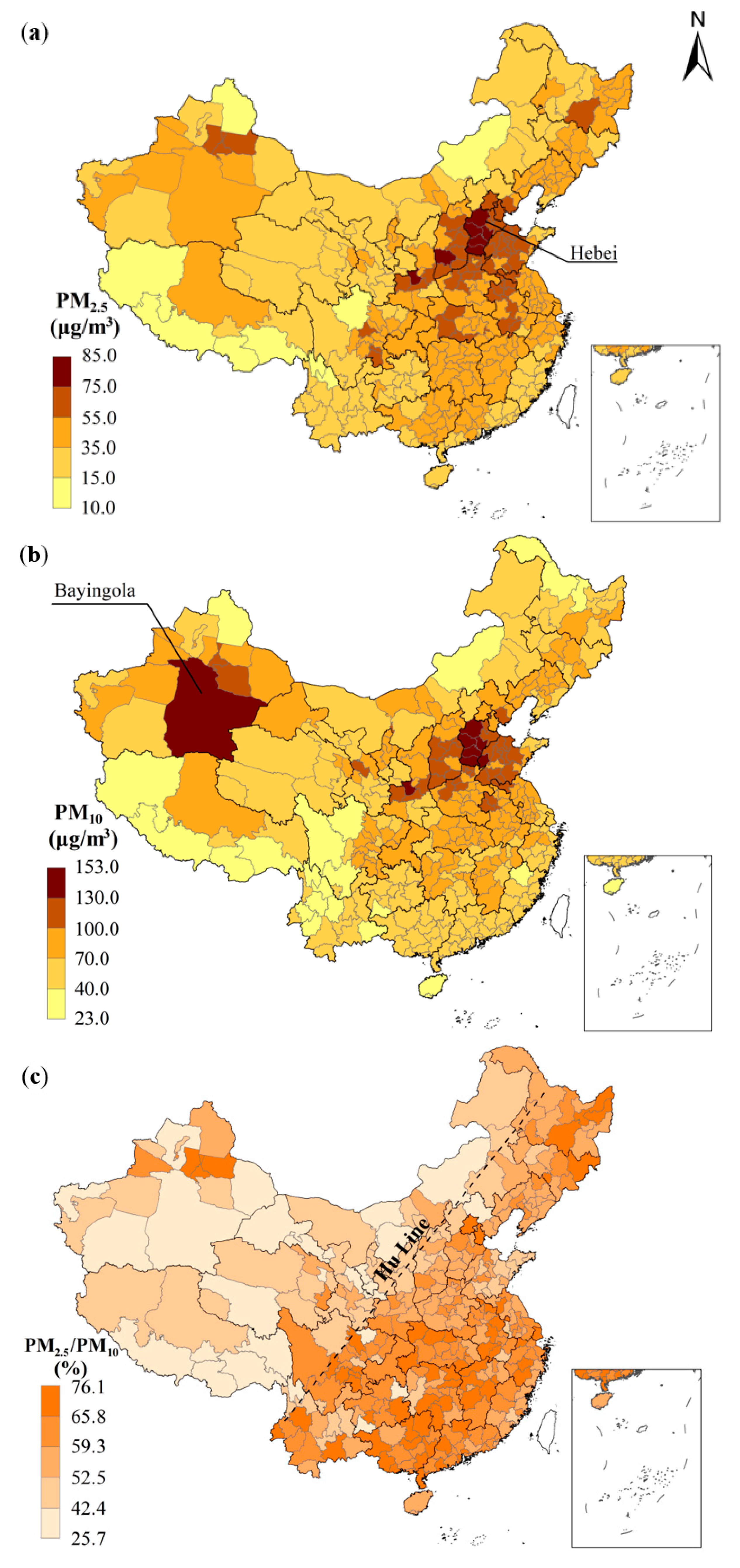
3.1. Spatial Variation of PM and Explanatory Variables

Table 2 shows the characteristics of the different variables, including PM2.5, PM10, PM2.5/PM10, precipitation, wind speed, population density, GDP density, and PBUA. The PM2.5 concentrations across Chinese mainland in 2017 ranged from 10.0 to 84.9 μg/m3, with an average value of 41.8 μg/m3. The annual-averaged value exceeded the national level II standard (<35 μg/m3) of PM2.5, according to the Environmental Air Quality Standard of China (GB3095-2012), and interim target 1 (IT-1) of the WHO Air Quality Guideline [40]. The PM10 concentrations ranged from 23.3 to 152.9 μg/m3, with an average value of 72.3 μg/m3. This value also failed to meet the level II standard of GB3095-2012 and the WHO Air Quality Guideline IT-1 (<70 μg/m3). Additionally, the PM2.5/PM10 ranged from 25.7% to 76.1%, with an average value of 56.5%. It is important to note that the PM2.5/PM10 values in Canada (average: 49%) [41], São Paulo state in Brazil (44.3%) [42], and the U.S. (ranged from 41.7% to 47.1% from 2014 to 2017) [43] were quite a bit lower than that in China; however, the corresponding values in India (ranged from 51.4% to 77.1% from 2014 to 2017) [43], and Iran (61.7%) [44] were similar to that in China. Furthermore, PM2.5 and PM10 can be summarized to have natural and anthropogenic sources, including dust (desert, road, and mineral), sea salt, traffic emission, coal combustion, industrial emission, biomass burning, and secondary inorganic aerosols [40,45,46]. Particles of secondary inorganic aerosols are the main source of PM2.5, and coal combustion is a major anthropogenic source of PM2.5, which has been reported in Beijing [46] and Chengdu [45]. Meanwhile, re-suspended dust has been considered the major source of ambient PM10 [16,46,47].
The spatial distribution of annual-averaged PM2.5, PM10, and PM2.5/PM10 concentrations are shown in Figure 1a–c. These figures show that annual-averaged PM2.5 concentrations of 119 (35.4%) cities satisfied the level II standard, while nine (2.7%) cities satisfied the level I standard (<15 μg/m3), which were mainly located in Tibet. Figure 1b shows that the PM10 concentrations of 167 (49.7%) cities were lower than the level II standard for PM10, while 23 (6.9%) cities met the level I standard for PM10 (<40 μg/m3). The area with the highest PM2.5 concentration was Hebei province, which was followed by its surrounding cities, such as Beijing, Tianjin, and cities in Shandong, Shanxi, and Henan provinces. The spatial characteristics of the highest PM10 concentration were similar to its PM2.5 counterpart; however, PM10 in the Bayingolin Mongolian Autonomous Prefecture in Xinjiang exhibited a considerably higher concentration. The lowest values of PM2.5 and PM10 concentrations were mainly observed in the southwest region of China. A large desert area is observed in northwest China, especially the Taklimakan Desert in Xinjiang; it is the largest desert in China (Figure 1d). As dust contributes much more to PM10 than PM2.5, Bayingolin had a high PM10 concentration.
In addition, the distribution of PM2.5/PM10 showed higher values in the southeast region as compared to that in the northwest region (Figure 1c). The boundary between low and high values was quite consistent with the Hu line, which is the line that categorizes the population density of China [48]. The Hu line has been regarded as one of the greatest geographical discoveries in China because it reveals the significant spatial relationship between human activity and the natural environment [49], highlighting the different responses of PM2.5 and PM10 to human activity and the natural environment.
To address severe air pollution issues and protect public health, the State Council of China promulgated the Action Plan of Air Pollution Prevention and Control (2013–2017) [50]. The PM2.5 and PM10 concentrations in 2017 decreased nationwide by 34.7% and 22.7% as compared to their 2013 levels, respectively [51]. This was particularly true for the PM2.5 and PM10 concentrations in the Beijing-Tianjin-Hebei region, which were reduced by 39.6% and 37.6% as compared to their 2013 levels, respectively [25,51]; this region is the most polluted region of China. In addition, there was a non-significant decrease in PM2.5/PM10 concentrations from 2013 to 2017 [51]. It is evident that the action plan is successful; however, 64.6% and 50.3% of the cities exhibited annual mean PM2.5 and PM10 concentrations that exceeded the threshold of the Chinese level II standard (GB3095-2012) and the WHO Air Quality Guideline IT-1, respectively. Although Fan et al. [52] indicated that cities with higher PM2.5 concentrations tend to experience a faster reduction in haze pollution, PM pollution in Hebei province remained the most serious. Therefore, continuous and effective emission control measures are still a high priority [53].
There is a big discrepancy in the natural and socioeconomic conditions across China. The annual precipitation across China is shown in Figure S1a; it ranged from 52.4 to 2718.4 mm on average. A high annual precipitation was mainly observed in the cities of Guangxi, Jiangxi, Hainan, and Guangdong province, which are located in southern China. A low precipitation was predominantly detected in the cities of Xinjiang, Gansu province, and Inner Mongolia, which are located in northern or northwest China. Figure S1b shows the spatial distribution of the annual average wind speed; the high wind speed mainly occurred in cities of the coastal, northwestern, and Tibetan regions. Vegetation distribution is controlled by hydrothermal conditions, as shown in Figure S1c; the NDVI in the southeast region was higher than that in the northwest region. Socioeconomic levels across Chinese mainland are shown in Figure S1d–f; cities with high population density, GDP density, and PBUA were all mainly found in the eastern coastal area, among which the cities with high population density were also found in central China. In contrast, the economic level of western China is relatively underdeveloped.

3.2. The Response of PM to Local Environment and Neighboring Pollution

Results of Moran’s I test showed that there was a significant autocorrelation for PM2.5 (0.68, p < 0.001), PM10 (0.69, p < 0.001), and PM2.5/PM10 (0.54, p < 0.001), indicating a spatial regression model would be more appropriate than OLS. The correlations between socioeconomic factors were very high (r = 0.73–0.95) (Figure S2), which implies that these three variables need to be incorporated into the model separately to avoid collinearity (Table S1).
Based on the results obtained with OLS for PM2.5 and PM10, precipitation and wind speed were found to have a significant negative correlation with PM2.5 and PM10, while population density, GDP density, and PBUA had a positive correlation with them. In addition, NDVI was found to have a significant relation to PM2.5 in most OLS models, while the coefficients of NDVI in models for PM10 were quite complicated. The result of four OLS models indicated that the socioeconomic impact on PM2.5 and PM10 levels was in the following order: population density > GDP density > PBUA (Table S1).
Therefore, population density was incorporated into SLM and SEM (Table 3). For PM2.5, PM10, and PM2.5/PM10, we found that the fitting coefficients (R2) of the spatial regression model (SLM, SEM) were higher than those of the OLS model, while the AIC value of the spatial regression model was lower than that of OLS. Further, SLM and SEM could remove the spatial autocorrelation of residuals. From Table 3, a similar correlation was observed in SLM and SEM, but the absolute values of most coefficients were lower than OLS. Moreover, the lagged term of the SLM showed a significant positive relation to PM2.5 (p < 0.001); this indicated that the air quality was not only affected by environmental and socioeconomic factors within that city but was also influenced by the PM level of neighboring cities. The significant spatial error parameter (Lambda) of the SEM suggested that there were unforeseen spatially autocorrelated variables that could affect PM levels. In addition, the coefficient value that indicates the lagged term was the most important factor for the PM2.5 and PM10 concentrations, suggesting the transport of pollutants emitted from neighboring regions was the major source of local PM on a national scale. Consistently, the major contribution of regional transportation to PM has been emphasized in previous studies [54,55]. More specifically, the contribution of regional transportation to PM2.5 was slightly higher than PM10, which may be due to smaller particulates being more easily transported to adjacent areas.
Moreover, based on the results of the four OLS models for PM2.5/PM10 (Table S1), population density, GDP density, and PBUA had an approximately positive influence on PM2.5/PM10. Precipitation and NDVI had a positive correlation with PM2.5/PM10, and all coefficients of wind speed were not significant. That is, population density, GDP density, PBUA, precipitation, and NDVI had different levels of influence on PM2.5 and PM10, while wind speed had a similar influence on them. Among local variables, the coefficient of NDVI was the largest, similar to that of population density, suggesting vegetation and human distribution both have a remarkably different impact on PM2.5 and PM10. Additionally, there was a significant lag term of PM2.5/PM10 in SLM. Similarly, the Lambda of the SEM also had a significant positive relation to PM2.5/PM10.
In addition, the absolute values of the coefficient of OLS were higher than those of SLM and SEM, indicating that the effect of variables in the OLS regression model was overestimated. Based on the coefficient of PM, precipitation had a greater influence on PM10 than on PM2.5; precipitation was the dominant variable that affected the dispersion of PM10. Population density was the most important local factor for the PM concentrations and played a more important role in PM2.5 than that in PM10. The higher population density as well as increased housing, electricity, and transport demands are direct causes of haze pollution [7], more fine particles were generated compared with coarse particles. Therefore, human activities are more likely to affect PM2.5 than PM10, which is consistent with previous studies [45,46]. Most OLS showed that NDVI had a significant positive relation to PM2.5, while only one OLS model showed that NDVI has a positive relation to PM10. This may be due to the place with higher NDVI, also with higher human activities, and PM2.5 is more susceptible to human activities. Moreover, vegetation plays an important role in reducing soil wind erosion because vegetation reduces wind speed near the soil surface and fixes the soil through roots, thereby inhibiting the resuspension of the settled dust [56,57,58]. The role of vegetation in reducing resuspended dust offsets the role of human activities in increasing PM10 on a national scale. This may be the reason there was no strong negative correlation between NDVI and PM10, as observed from the spatial regression model based on all cities in Chinese mainland. In summary, the impact of variables on PM was in the following order: regional transportation > population density > precipitation > wind speed > NDVI. Population density had a greater impact on PM10 than PM2.5, while precipitation had the opposite effect.

3.3. Varying Response of PM Level to Natural and Socioeconomic Conditions

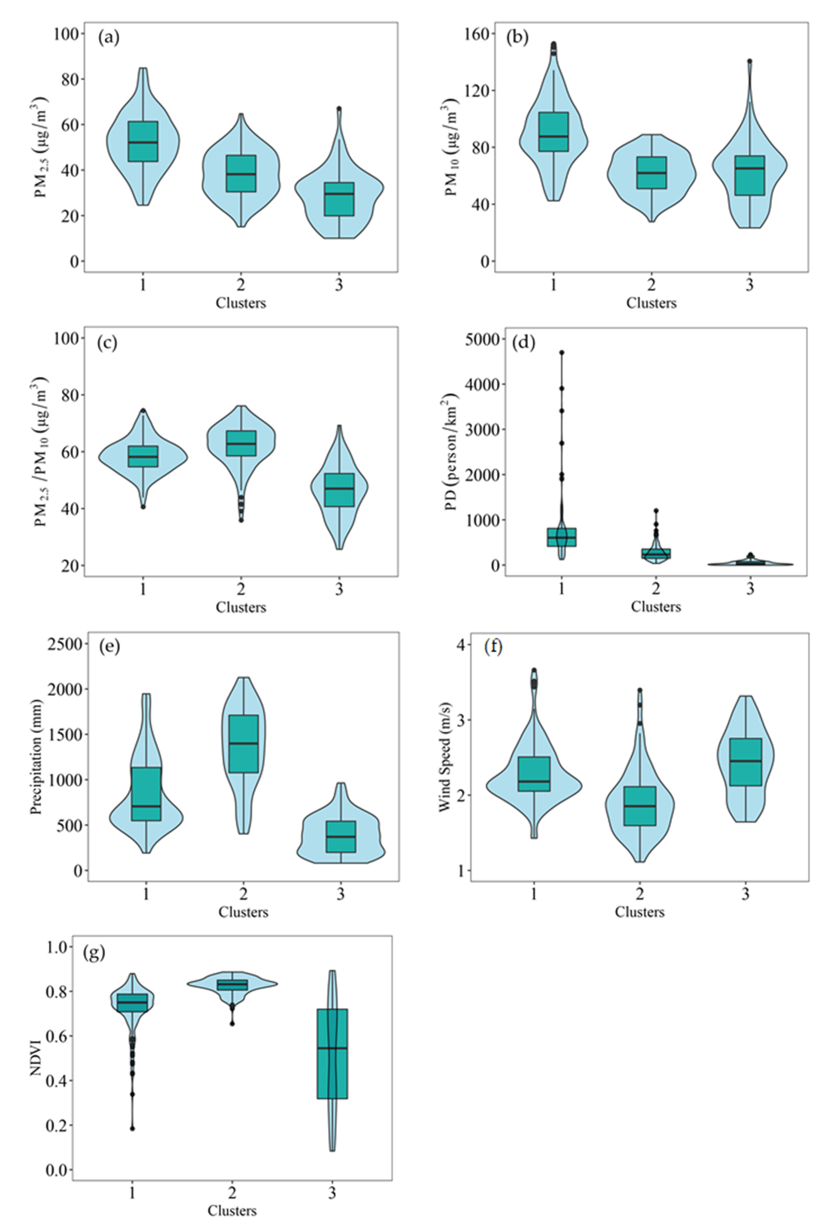
3.3.1. Spatial Character of Each Cluster

The sum of the squared distance within the cluster decreased slowly after three clusters; thus, the optimal number of clusters was determined to be three. Then, the cities in China were divided into three groups based on PM levels as well as natural and socioeconomic conditions (Figure 2). Group 1 (G1) included 129 cities, which were mainly located in or around Hebei province, including the Northeast Plain and North China Plain. Over 60% of provincial capitals and municipal cities were included in G1. Group 2 (G2) included 139 cities that were mostly located in southern China, such as Sichuan, Guangxi, and Yunnan provinces; meanwhile, a small number of cities were located in the northeast region of China, including the cities in Heilongjiang and Jilin provinces. Group 3 (G3) included 68 cities, which were mainly found in the western region, such as the cities in Inner Mongolia, Xinjiang, Tibet, and Qinghai provinces.
Compared to the cities in the other two groups, cities in G1 with the highest PM2.5 and PM10 levels were the most developed with increased socioeconomic levels (Figure 3). The median PM2.5 and PM10 values of G1 were 52.1 and 90.4 μg/m3 (Table S2), respectively. The median population density of G1 (605.1 persons/km2) was 2.6 and 23.1 times the cities in G2 and G3, respectively. There is a huge difference in the distribution of the population in China, particularly the population in G1, which showed remarkable variability (Figure 3d). Cities in G2 exhibit the lowest PM10 levels (61.9 μg/m3) with minimum variability and range (Figure 3b), owing to significant precipitation (Figure 3e) and dense vegetation (Figure 3g). Consequently, the median PM2.5/PM10 in G2 was the highest (62.7%) (Figure 3c), which indicated that human activities are the major source of PM pollution in G2. Compared to G1 (the most polluted region) and G2 (southern China), sparser populations occurred in G3 (western China) (Figure 3d) wherein the climate is relatively arid and there is a large area of desert and plateau. More specifically, the annual precipitation in many regions of G3 was less than 500 mm (Figure 3e). With the most undeveloped socioeconomic level, G3 exhibited the lowest PM2.5 concentration (29.5 μg/m3); meanwhile, the median PM10 value (65.2 μg/m3) in western China was the second; however, this was because fugitive dust emissions tend to occur more easily in western China, as G3 with the highest wind speed (Figure 3f) and the lowest NDVI (Figure 3g). The PM2.5/PM10 concentration in the western region was the lowest (47.0%), which suggested that human activities had less effect on PM pollution and that dust is the major source of PM pollution in western China.

3.3.2. Varying Driving Forces of PM in Each Cluster

SEM was applied to identify the driving forces of the PM levels in each cluster (Table 4), as SEM performed better than OLS and SLM in each cluster (the highest R2 and lowest AIC). Population density was selected as the variable that represents the socioeconomic level because it functioned as the most influential local variable for the PM level, as observed from the global regression results. Given that precipitation and NDVI exhibited a high correlation (r = 0.81) in G3 (Figure S2), they were incorporated into the model separately.
In the most polluted region (G1), precipitation and wind speed had a significant negative impact on the PM level. It is worth noting that a decoupling relationship exists between population density and PM level in G1. Industrial activities were considered the dominant driver of fine particle concentrations in the Beijing-Tianjin-Hebei region [59]. Hebei, Henan, Shandong, and Jiangsu provinces exhibited high degrees of manufacturing agglomeration, increased energy consumption, and excessive pollutant emissions, which can lead to heavy smog pollution [7]. Given G1 is the most developed region, and there are many industrial cities, the city with the highest pollution emission was mainly located in Hebei province rather than the most densely populated city. Consequently, population density as an indirect influential factor failed to show a significant correlation with PM2.5 concentrations.
In southern China (G2), population density was the most influential variable for the PM level. Precipitation had a negative impact on PM2.5 and PM10, while wind speed only had a significant impact on PM10. In western China (G3), population density was the most influential local variable for PM2.5, while precipitation significantly affected PM10. In contrast to G1, the impact of the dispersion caused by wind speed on PM2.5 concentration was slightly smaller in G2 and G3. This probably because G2 lies to south of the G1, it would be more susceptible to monsoons that vary in wind direction over the course of a year than to wind speed. Moreover, cities in G3 exhibit the lowest precipitation and vegetation coverage and the highest wind speed; thus, the effect of high wind speed on the evacuation of PM was probably offset due to the floating dust that it causes. In addition to precipitation, NDVI was also found to have a significant negative relation to PM10. In addition, most of the Lambda values were non-significant in G3, while significant autocorrelation of unforeseen circumstances existed in G1 and G2, this may be because our research was based on prefecture-level cities, while cities in western China exhibit a larger area. In summary, the regional scale regression result highlighted the dispersion effect of precipitation on PM concentrations in the most polluted and western regions, especially on PM10. Furthermore, vegetation covering can significantly reduce PM10 in western China, which is the region that comprises a large area of desert and plateau; this is because vegetation plays a major role in windbreak and sand fixation.

4. Conclusions

This study presented the spatial distributions of PM2.5 and PM10 concentrations across Chinese mainland in 2017. From the perspective of local and neighboring effects, the driving forces of these PMs were also investigated. Although PM pollution has improved in recent years in China, nearly two-thirds or half of the cities still exceeded the level II standard of GB3095-2012 for annual PM2.5 and PM10 concentrations, respectively. The area with the highest PM2.5 and PM10 concentrations was mainly located in Hebei province, which was followed by the corresponding concentrations in its surrounding cities. In addition, the distribution of PM2.5/PM10 showed higher values in the southeast region than in the northwest region, and the boundary line between the low and high values was quite consistent with the Hu line.
Global spatial regression results revealed that the neighboring air pollution level played a dominant role in the spatial variation of PM2.5 and PM10 concentrations in Chinese mainland, while population density was the most influential local variable for PM2.5 and PM10. Additionally, precipitation was the most influential dispersion variable, followed by wind speed. The influence of socioeconomic factors and neighboring pollution on PM2.5 was greater than that on PM10, while precipitation was more influential for PM10. In addition, precipitation, NDVI, and socioeconomic factors had a positive correlation with PM2.5/PM10.
Cities with relevant characteristics were clustered into a group with a k-means cluster. Population density was the most influential variable for PM in southern and western China. In addition, the dispersion effect of the precipitation was highlighted in the region with heavy PM pollution and western China, especially on PM10. In addition to precipitation, NDVI also had a significant reducing effect on PM10 in western China. Therefore, a targeted strategy needs to be formulated for reducing regional air pollution by considering the local environment and spatial spillover effect.
Limited by the lack of nationwide data on direct sources of PM pollution, population density, GDP density, and PBUA were selected as the indirect factors in this study. A non-significant relation to PM in regions with dense industrial structures may lead to an underestimation of the influence of human activities on PM concentrations.

Supplementary Materials

The following supporting information can be downloaded at: https://www.mdpi.com/article/10.3390/atmos14010186/s1, Figure S1: Spatial variation of independent variables across Chinese mainland; Figure S2: Spearman correlation between variables of each cluster; Table S1: Regression results of PM2.5, PM10, and PM2.5/PM10 based on OLS; Table S2: Summary of the characteristics of variables in each cluster.

Author Contributions

Conceptualization, methodology, writing—review and editing, C.G. and M.L.; formal analysis, writing—original draft preparation, visualization, C.G.; supervision, M.L.; funding acquisition, M.L. and C.G. All authors have read and agreed to the published version of the manuscript.

Funding

This research was funded by the National Natural Science Foundation of China (grant number 41977399), and the Science Foundation of Hengyang Normal University (grant number 2022QD16).

Institutional Review Board Statement

Not applicable.

Informed Consent Statement

Not applicable.

Data Availability Statement

Data sharing is not applicable to this article.

Acknowledgments

The authors would like to thank the “National Urban Air Quality Real Time Release Platform” for providing air pollution data, and the “Resource and Environment Data Cloud Platform” for providing socioeconomic, land use, and vegetation data.

Conflicts of Interest

The authors declare no conflict of interest.

References

  1. Feng, H.; Zou, B.; Wang, J.; Gu, X. Dominant variables of global air pollution-climate interaction: Geographic insight. Ecol. Indic. 2019, 99, 251–260. [Google Scholar] [CrossRef]
  2. Lacressonnière, G.; Peuch, V.-H.; Vautard, R.; Arteta, J.; Déqué, M.; Joly, M.; Josse, B.; Marécal, V.; Saint-Martin, D. European air quality in the 2030s and 2050s: Impacts of global and regional emission trends and of climate change. Atmos. Environ. 2014, 92, 348–358. [Google Scholar] [CrossRef]
  3. Shiraiwa, M.; Li, Y.; Tsimpidi, A.P.; Karydis, V.A.; Berkemeier, T.; Pandis, S.N.; Lelieveld, J.; Koop, T.; Pöschl, U. Global distribution of particle phase state in atmospheric secondary organic aerosols. Nat. Commun. 2017, 8, 15002. [Google Scholar] [CrossRef] [PubMed] [Green Version]
  4. Zhang, R. Warming boosts air pollution. Nat. Clim. Chang. 2017, 7, 238–239. [Google Scholar] [CrossRef]
  5. Lelieveld, J.; Klingmüller, K.; Pozzer, A.; Pöschl, U.; Fnais, M.; Daiber, A.; Münzel, T. Cardiovascular disease burden from ambient air pollution in Europe reassessed using novel hazard ratio functions. Eur. Heart J. 2019, 40, 1590–1596. [Google Scholar] [CrossRef] [Green Version]
  6. Li, J.; Han, X.; Jin, M.; Zhang, X.; Wang, S. Globally analysing spatiotemporal trends of anthropogenic PM2.5 concentration and population’s PM2.5 exposure from 1998 to 2016. Environ. Int. 2019, 128, 46–62. [Google Scholar] [CrossRef]
  7. Cheng, Z.; Li, L.; Liu, J. Identifying the spatial effects and driving factors of urban PM2.5 pollution in China. Ecol. Indic. 2017, 82, 61–75. [Google Scholar] [CrossRef]
  8. Yuan, M.; Song, Y.; Huang, Y.; Hong, S.; Huang, L. Exploring the Association between Urban Form and Air Quality in China. J. Plan. Educ. Res. 2018, 38, 413–426. [Google Scholar] [CrossRef]
  9. Zhao, S.; Liu, S.; Hou, X.; Beazley, R.; Sun, Y. Identifying the contributions of multiple driving forces to PM10-2.5 pollution in urban areas in China. Sci. Total Environ. 2019, 663, 361–368. [Google Scholar] [CrossRef]
  10. Mahara, G.; Wang, C.; Yang, K.; Chen, S.; Guo, J.; Gao, Q.; Wang, W.; Wang, Q.; Guo, X. The Association between Environmental Factors and Scarlet Fever Incidence in Beijing Region: Using GIS and Spatial Regression Models. Int. J. Environ. Res. Public Health 2016, 13, 1083. [Google Scholar] [CrossRef]
  11. Jiang, C.; Wang, H.; Zhao, T.; Li, T.; Che, H. Modeling study of PM2.5 pollutant transport across cities in China’s Jing-Jin-Ji region during a severe haze episode in December 2013. Atmos. Chem. Phys. 2015, 15, 5803–5814. [Google Scholar] [CrossRef] [Green Version]
  12. WHO. Particulate Matter Air Pollution: How It Harms Health. 2005. Available online: https://www.eea.europa.eu/themes/air/health-impacts-of-air-pollution (accessed on 15 April 2020).
  13. Chen, R.; Yin, P.; Meng, X.; Liu, C.; Wang, L.; Xu, X.; Ross, J.A.; Tse, L.A.; Zhao, Z.; Kan, H.; et al. Fine Particulate Air Pollution and Daily Mortality. A Nationwide Analysis in 272 Chinese Cities. Am. J. Respir. Crit. Care Med. 2017, 196, 73–81. [Google Scholar] [CrossRef]
  14. Samoli, E.; Analitis, A.; Touloumi, G.; Schwartz, J.; Anderson, H.R.; Sunyer, J.; Bisanti, L.; Zmirou, D.; Vonk, J.M.; Pekkanen, J.; et al. Estimating the Exposure–Response Relationships between Particulate Matter and Mortality within the APHEA Multicity Project. Environ. Health Perspect. 2005, 113, 88–95. [Google Scholar] [CrossRef] [Green Version]
  15. Goudie, A.S. Desert dust and human health disorders. Environ. Int. 2014, 63, 101–113. [Google Scholar] [CrossRef] [PubMed]
  16. Rodríguez, S.; Querol, X.; Alastuey, A.; Viana, M.; Alarcón, M.; Mantilla, E.; Ruiz, C. Comparative PM10–PM2.5 source contribution study at rural, urban and industrial sites during PM episodes in Eastern Spain. Sci. Total Environ. 2004, 328, 95–113. [Google Scholar] [CrossRef]
  17. Piras, G.; Pini, F.; Garcia, D.A. Correlations of PM10 concentrations in urban areas with vehicle fleet development, rain precipitation and diesel fuel sales. Atmos. Pollut. Res. 2019, 10, 1165–1179. [Google Scholar] [CrossRef]
  18. Gao, C.; Li, S.; Liu, M.; Zhang, F.; Achal, V.; Tu, Y.; Zhang, S.; Cai, C. Impact of the COVID-19 pandemic on air pollution in Chinese megacities from the perspective of traffic volume and meteorological factors. Sci. Total Environ. 2021, 773, 145545. [Google Scholar] [CrossRef] [PubMed]
  19. Kim, K.-H.; Kim, M.-Y.; Hong, S.; Youn, Y.; Hwang, S.-J. The effects of wind speed on the relative relationships between different sized-fractions of airborne particles. Chemosphere 2005, 59, 929–937. [Google Scholar] [CrossRef] [PubMed]
  20. Xiang, Y.; Zhang, T.; Liu, J.; Lv, L.; Dong, Y.; Chen, Z. Atmosphere boundary layer height and its effect on air pollutants in Beijing during winter heavy pollution. Atmos. Res. 2019, 215, 305–316. [Google Scholar] [CrossRef]
  21. Wu, C.-D.; Chen, Y.-C.; Pan, W.-C.; Zeng, Y.-T.; Chen, M.-J.; Guo, Y.L.; Lung, S.-C.C. Land-use regression with long-term satellite-based greenness index and culture-specific sources to model PM2.5 spatial-temporal variability. Environ. Pollut. 2017, 224, 148–157. [Google Scholar] [CrossRef]
  22. Mamtimin, B.; Meixner, F.X. Air pollution and meteorological processes in the growing dryland city of Urumqi (Xinjiang, China). Sci. Total Environ. 2011, 409, 1277–1290. [Google Scholar] [CrossRef]
  23. Zhang, W.; Wang, H.; Zhang, X.; Peng, Y.; Zhong, J.; Wang, Y.; Zhao, Y. Evaluating the contributions of changed meteorological conditions and emission to substantial reductions of PM2.5 concentration from winter 2016 to 2017 in Central and Eastern China. Sci. Total Environ. 2020, 716, 136892. [Google Scholar] [CrossRef]
  24. Zhao, S.; Yu, Y.; Qin, D.; Yin, D.; Dong, L.; He, J. Analyses of regional pollution and transportation of PM2.5 and ozone in the city clusters of Sichuan Basin, China. Atmos. Pollut. Res. 2019, 10, 374–385. [Google Scholar] [CrossRef]
  25. Chen, X.; Li, F.; Zhang, J.; Zhou, W.; Wang, X.; Fu, H. Spatiotemporal mapping and multiple driving forces identifying of PM2.5 variation and its joint management strategies across China. J. Clean. Prod. 2020, 250, 119534. [Google Scholar] [CrossRef]
  26. Yang, X.; Wang, S.; Zhang, W.; Zhan, D.; Li, J. The impact of anthropogenic emissions and meteorological conditions on the spatial variation of ambient SO2 concentrations: A panel study of 113 Chinese cities. Sci. Total Environ. 2017, 584, 318–328. [Google Scholar] [CrossRef]
  27. Hutchinson, M.F.; Xu, T. ANUSPLIN VERSION 4.4. USER GUIDE; The Australian National University, Centre for Resource and Environmental Studies: Canberra, Australia, 2013. [Google Scholar]
  28. Yin, C.; Yuan, M.; Lu, Y.; Huang, Y.; Liu, Y. Effects of urban form on the urban heat island effect based on spatial regression model. Sci. Total Environ. 2018, 634, 696–704. [Google Scholar] [CrossRef]
  29. Tian, W.; Song, J.; Li, Z. Spatial regression analysis of domestic energy in urban areas. Energy 2014, 76, 629–640. [Google Scholar] [CrossRef]
  30. Ahn, K.-H.; Palmer, R. Regional flood frequency analysis using spatial proximity and basin characteristics: Quantile regression vs. parameter regression technique. J. Hydrol. 2016, 540, 515–526. [Google Scholar] [CrossRef]
  31. Fischer, M.; Wang, J. Spatial Data Analysis: Models, Methods and Techniques; Springer: Berlin/Heidelberg, Germany, 2011. [Google Scholar]
  32. Cliff, A.D.; Ord, J.K. Spatial Processes: Models & Applications; Taylor & Francis: Abingdon, UK, 1981. [Google Scholar]
  33. Kumari, M.; Sarma, K.; Sharma, R. Using Moran’s I and GIS to study the spatial pattern of land surface temperature in relation to land use/cover around a thermal power plant in Singrauli district, Madhya Pradesh, India. Remote Sens. Appl. Soc. Environ. 2019, 15, 100239. [Google Scholar] [CrossRef]
  34. Austin, E.; Coull, B.A.; Zanobetti, A.; Koutrakis, P. A framework to spatially cluster air pollution monitoring sites in US based on the PM2.5 composition. Environ. Int. 2013, 59, 244–254. [Google Scholar] [CrossRef]
  35. Chen, Z.; Chen, D.; Xie, X.; Cai, J.; Zhuang, Y.; Cheng, N.; He, B.; Gao, B. Spatial self-aggregation effects and national division of city-level PM2.5 concentrations in China based on spatio-temporal clustering. J. Clean. Prod. 2019, 207, 875–881. [Google Scholar] [CrossRef]
  36. Govender, P.; Sivakumar, V. Application of k-means and hierarchical clustering techniques for analysis of air pollution: A review (1980–2019). Atmos. Pollut. Res. 2020, 11, 40–56. [Google Scholar] [CrossRef]
  37. Kahya, C.; Balcik, F.B.; Oztaner, Y.B.; Ozcomak, D.; Seker, D.Z. Spatio-temporal analysis of PM2.5 over Marmara region, Turkey. Fresen. Environ. Bull. 2017, 26, 310–317. [Google Scholar]
  38. Zhao, S.; Yu, Y.; Yin, D.; He, J.; Liu, N.; Qu, J.; Xiao, J. Annual and diurnal variations of gaseous and particulate pollutants in 31 provincial capital cities based on in situ air quality monitoring data from China National Environmental Monitoring Center. Environ. Int. 2016, 86, 92–106. [Google Scholar] [CrossRef] [PubMed]
  39. Dabbura, I. K-Means Clustering: Algorithm, Applications, Evaluation Methods, and Drawbacks. 2018. Available online: https://towardsdatascience.com/k-means-clustering-algorithm-applications-evaluation-methods-and-drawbacks-aa03e644b48a (accessed on 20 April 2020).
  40. WHO. WHO Air Quality Guidelines Global Update 2005; The Regional Office for Europe of the World Health Organization: Copenhagen, Denmark, 2005; p. 278.
  41. Brook, J.R.; Dann, T.F.; Burnett, R.T. The Relationship Among TSP, PM10, PM2.5, and Inorganic Constituents of Atmospheric Participate Matter at Multiple Canadian Locations. J. Air Waste Manag. Assoc. 1997, 47, 2–19. [Google Scholar] [CrossRef] [Green Version]
  42. Franzin, B.T.; Guizellini, F.C.; Babos, D.; Hojo, O.; Pastre, I.A.; Marchi, M.R.; Fertonani, F.L.; Oliveira, C. Characterization of atmospheric aerosol (PM10 and PM2.5) from a medium sized city in São Paulo state, Brazil. J. Environ. Sci. 2020, 89, 238–251. [Google Scholar] [CrossRef]
  43. Yang, X.; Jiang, L.; Zhao, W.; Xiong, Q.; Zhao, W.; Yan, X. Comparison of Ground-Based PM2.5 and PM10 Concentrations in China, India, and the US. Int. J. Environ. Res. Public Health 2018, 15, 1382. [Google Scholar] [CrossRef] [Green Version]
  44. Omidi Khaniabadi, Y.; Sicard, P.; Omidi Khaniabadi, A.; Mohammadinejad, S.; Keishams, F.; Takdastan, A.; Najafi, A.; De Marco, A.; Daryanoosh, M. Air quality modeling for health risk assessment of ambient PM10, PM2.5 and SO2 in Iran. Hum. Ecol. Risk Assess. 2019, 25, 1298–1310. [Google Scholar] [CrossRef]
  45. Tao, J.; Gao, J.; Zhang, L.; Zhang, R.; Che, H.; Zhang, Z.; Lin, Z.; Jing, J.; Cao, J.; Hsu, S.-C. PM2.5 pollution in a megacity of southwest China: Source apportionment and implication. Atmos. Meas. Tech. 2014, 14, 8679–8699. [Google Scholar] [CrossRef] [Green Version]
  46. Wang, H.; Zhuang, Y.; Wang, Y.; Sun, Y.; Yuan, H.; Zhuang, G.; Hao, Z. Long-term monitoring and source apportionment of PM2.5/PM10 in Beijing, China. J. Environ. Sci. 2008, 20, 1323–1327. [Google Scholar] [CrossRef]
  47. Bi, X.; Feng, Y.; Wu, J.; Wang, Y.; Zhu, T. Source apportionment of PM10 in six cities of northern China. Atmos. Environ. 2007, 41, 903–912. [Google Scholar] [CrossRef]
  48. Hu, H. Distribution of China’s population: Accompanying charts and density map. Acta Geogr. Sin. 1935, 2, 33–74. [Google Scholar]
  49. Qi, W.; Liu, S.; Zhao, M.; Liu, Z. China’s different spatial patterns of population growth based on the “Hu Line”. J. Geogr. Sci. 2016, 26, 1611–1625. [Google Scholar] [CrossRef]
  50. Central People’s Government of the People’s Republic of China. The Report Released by the National Bureau of Statistics—China’s Urbanization Rate Has Increased Significantly in the Past 70 Years. 2019. Available online: http://www.gov.cn/shuju/2019-08/16/content_5421576.htm (accessed on 31 August 2020).
  51. Wang, Y.; Li, W.; Gao, W.; Liu, Z.; Tian, S.; Shen, R.; Ji, D.; Wang, S.; Wang, L.; Tang, G.; et al. Trends in particulate matter and its chemical compositions in China from 2013–2017. Sci. China Earth Sci. 2019, 62, 1857–1871. [Google Scholar] [CrossRef]
  52. Fan, X.; Xu, Y. Convergence on the haze pollution: City-level evidence from China. Atmos. Pollut. Res. 2020, 11, 141–152. [Google Scholar] [CrossRef]
  53. Zhang, Q.; Zheng, Y.; Tong, D.; Shao, M.; Wang, S.; Zhang, Y.; Xu, X.; Wang, J.; He, H.; Liu, W.; et al. Drivers of improved PM2.5 air quality in China from 2013 to 2017. Proc. Natl. Acad. Sci. USA 2019, 116, 24463–24469. [Google Scholar] [CrossRef] [Green Version]
  54. Chen, D.; Liu, X.; Lang, J.; Zhou, Y.; Wei, L.; Wang, X.; Guo, X. Estimating the contribution of regional transport to PM2.5 air pollution in a rural area on the North China Plain. Sci. Total Environ. 2017, 583, 280–291. [Google Scholar] [CrossRef]
  55. Hu, W.; Zhao, T.; Bai, Y.; Kong, S.; Xiong, J.; Sun, X.; Lu, H. Importance of regional PM2.5 transport and precipitation washout in heavy air pollution in the Twain-Hu Basin over Central China: Observational analysis and WRF-Chem simulation. Sci. Total Environ. 2021, 758, 143710. [Google Scholar] [CrossRef]
  56. Li, J.; Ma, X.; Zhang, C. Predicting the spatiotemporal variation in soil wind erosion across Central Asia in response to climate change in the 21st century. Sci. Total Environ. 2020, 709, 136060. [Google Scholar] [CrossRef]
  57. Wu, Z.; Wang, M.; Zhang, H.; Du, Z. Vegetation and soil wind erosion dynamics of sandstorm control programs in the agro-pastoral transitional zone of northern China. Front. Earth Sci. 2019, 13, 430–443. [Google Scholar] [CrossRef]
  58. Yan, Y.; Xu, X.; Xin, X.; Yang, G.; Wang, X.; Yan, R.; Chen, B. Effect of vegetation coverage on aeolian dust accumulation in a semiarid steppe of northern China. Catena 2011, 87, 351–356. [Google Scholar] [CrossRef]
  59. Li, X.; Zhang, Q.; Zhang, Y.; Zheng, B.; Wang, K.; Chen, Y.; He, K. Source contributions of urban PM2.5 in the Beijing–Tianjin–Hebei region: Changes between 2006 and 2013 and relative impacts of emissions and meteorology. Atmos. Environ. 2015, 123, 229–239. [Google Scholar] [CrossRef]
Figure 1. Spatial distribution of annual-averaged PM levels in Chinese mainland; (a) Spatial distribution of PM2.5, (b) Spatial distribution of PM10, (c) Spatial distribution of PM2.5/ PM10, and (d) Spatial distribution of sandy land.
Atmosphere 14 00186 g001aAtmosphere 14 00186 g001b
Figure 2. Clustering spatial distribution of cities in the mainland of China.
Atmosphere 14 00186 g002
Figure 3. Variation in PM levels as well as natural and socioeconomic conditions in each cluster. (a) PM2.5 characteristic in each cluster, (b) PM10 characteristic in each cluster, (c) PM2.5/PM10 characteristic in each cluster, (d) PD (Population density) characteristic in each cluster, (e) Precipitation characteristic in each cluster, (f) Wind speed characteristic in each cluster, (g) NDVI characteristic in each cluster.
Atmosphere 14 00186 g003
Table 1. List of data sources used in the current study.
DataYearTime ResolutionSpatial ResolutionSource
Air pollution data20171 dayCityChina Air Quality Online Monitoring and Analysis Platform (https://www.aqistudy.cn/historydata/, accessed on 1 March 2020)
PM2.5, PM10
Meteorological factors20171 dayStationChina Meteorological Data Network (http://data.cma.cn/, accessed on 7 March 2020)
Precipitation wind speed
Vegetation Index20171 year1 km × 1 kmResource and Environment Data Cloud Platform (http://www.resdc.cn/Default.aspx, accessed on 10 January 2020)
NDVI
Socioeconomic factors20151 year1 km × 1 kmResource and Environment Data Cloud Platform (http://www.resdc.cn/Default.aspx, accessed on 3 December 2019)
PD, GDPD, PBUA
PD: population density; GDPD: gross domestic product density; PBUA: proportion of built-up area.
Table 2. Characteristics of PM and its influencing variables in China.
VariablesMinMaxSDMean
PM2.5 (μg/m3)10.084.914.641.8
PM10 (μg/m3)23.3152.924.172.3
PM2.5/PM10 (%)25.776.19.456.5
Precipitation (mm)52.42718.41002.8538.5
Wind speed (m/s)1.13.80.52.3
NDVI0.080.90.20.7
PD (person/km2)0.34700.5513.5413.0
GDPD (10,000 yuan/km2)0.243,032.44558.62416.2
PBUA (%)038.53.61.7
SD: Standard deviation.
Table 3. Regression results of PM2.5, PM10, and PM2.5/PM10.
VariablesPM2.5PM10PM2.5/PM10
OLSSLMSEMOLSSLMSEMOLSSLMSEM
Precipitation−0.35 ***−0.14 ***−0.20 **−0.46 ***−0.19 ***−0.33 **0.24 ***0.16 ***0.24 ***
Wind speed−0.16 **−0.09 *−0.09−0.18 ***−0.10 **−0.12 *0.050.030.03
NDVI0.09 *0.010.12−0.06−0.04−0.0020.27 ***0.18 ***0.26 ***
log (PD)0.75 ***0.37 ***0.58 ***0.70 ***0.35 ***0.53 ***0.23 ***0.17 **0.21 ***
Lagged term 0.68 *** 0.67 *** 0.35 ***
constant0.10 *−0.0060.070.28 ***0.07 *0.23 ***0.16 ***0.080.18
Lambda 0.74 *** 0.73 *** 0.37 ***
R20.410.670.650.440.680.670.460.50.49
Adjusted R20.4 0.43 0.45
AIC−308.25−493.7−490.05−359.79−541.27−534.7−372.26−398.28−395.75
Moran I (residual)0.540.004−0.050.530.004−0.040.20.01−0.002
SD of Moran I (residual)14.79 ***0.18−1.1614.61 ***0.20 ***−1.035.41 ***0.360.03
Note: * p < 0.05, ** p < 0.01, *** p < 0.001; PD: population density; Lagged term: Lagged PM for nearby cities; Lambda: spatial error parameter in SEM; Bold: the most important variable. The standardization coefficients of socioeconomic factors without log conversion were also the most dominant local variables.
Table 4. SEM regression results of PM2.5 and PM10 in each cluster.
VariablesPM2.5PM10
G1G2G3-1G3-2G1G2G3-1G3-2
Precipitation−0.45 ***−0.11−0.31 **-−0.50 ***−0.26 ***−0.43 ***-
Wind speed−0.25 ***−0.06−0.06−0.01−0.19 *−0.25 *−0.10−0.04
NDVI0.27 **0.22-−0.130.100.13-−0.32 ***
log (PD)0.150.50 ***0.36 ***0.38 ***0.080.53 ***0.33 ***0.39 ***
constant0.43 ***0.150.26 **0.18 *0.56 ***0.45 **0.34 ***0.29 ***
Lambda0.55 ***0.67 ***0.280.35 *0.63 ***0.63 ***0.290.24
R20.580.420.300.240.620.460.410.38
AIC−118.36−113.76−41.98−37.37−150.13−91.28−58.98−56.35
Moran I (residual)−0.02−0.04−0.010.01−0.01−0.080.030.03
SD of Moran I (residual)−0.11−0.440.300.26−0.06−1.150.490.43
G3-1: NDVI was not included in the variables; G3-2: precipitation was not included in the variables.
Disclaimer/Publisher’s Note: The statements, opinions and data contained in all publications are solely those of the individual author(s) and contributor(s) and not of MDPI and/or the editor(s). MDPI and/or the editor(s) disclaim responsibility for any injury to people or property resulting from any ideas, methods, instructions or products referred to in the content.

