Abstract
The close proximity of crosswinds to airport runways presents great hazards to landing operations. As a result, an aircraft is susceptible to encountering a loss of control. Elevated levels of turbulence are commonly linked with strong crosswind speeds over the runway glide path. Therefore, it is imperative to evaluate the factors that impact crosswind speeds. The susceptibility of the runways at Hong Kong International Airport (HKIA) to severe crosswinds is well established. This study aimed to build a scaled model of HKIA, along with its surrounding terrain/buildings, within a TJ-3 ABL wind tunnel to compute the crosswind speeds under different wind directions over the runway glide path. Subsequently, utilizing the outcomes of the experiment, a cutting-edge local cascade ensemble (LCE) model was employed in conjunction with a tree-structured Parzen estimator (TPE) to evaluate the crosswind speed over the north runway glide path. The comparative analysis of the TPE-LCE model was also conducted with other machine learning models. The TPE-LCE model demonstrated superior predictive capabilities in comparison to alternative models, as assessed by MAE (0.490), MSE (0.381), RMSE (0.617), and R2 (0.855). The SHAP analysis, which utilized TPE-LCE predictions, revealed that two factors, specifically “Effect of Terrain/Buildings” and “Distance from Runway,” exhibiting noteworthy influence over the probability of encountering elevated crosswind speeds over the runway glide path. The optimal conditions for high-crosswind speeds were found to be characterized by the absence of nearby terrain features or structures, a smaller distance from HKIA’s north runway threshold, and with a wind direction ranging from 125 to 180 degrees.
1. Introduction
The crosswind refers to a wind vector that is orthogonal to the direction of travel of an aircraft. The impact of crosswind on air navigation is of the utmost importance, particularly during takeoff and landing, due to its potential to cause drift [1]. Parallel alignment with the wind during takeoff and landing procedures results in increased efficiency. The ground-speed of the aircraft is reduced, a shorter runway is required for takeoff, and the pilot has more time to make the necessary adjustments for a smooth landing. As the wind direction shifts to a perpendicular angle with respect to the runway, resulting in a crosswind scenario as depicted in Figure 1, the aircraft’s directional stability is impacted. In the event that a pilot neglects to adequately adjust for the presence of a crosswind, it is possible for the aircraft to deviate from the runway or for the landing gear to encounter a side load.
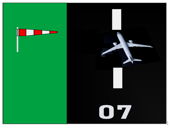
Figure 1.
Crosswind effect on the aircraft.
The process of safely landing an aircraft is regarded by many as one of the most challenging assignments within a pilot’s regular flight operations. To accomplish this task, pilots must skillfully maneuver the aircraft while consistently acknowledging and adjusting to changes in the immediate surroundings, such as air traffic control (ATC) restrictions and local weather patterns, among other factors. The second category commonly evokes considerable concern among pilots within the realm of civil aviation [2]. The occurrence of landing in a crosswind serves as a prominent illustration of how adverse weather conditions can intensify the complexity of an already challenging task. As the intensity of the crosswind increases, the pilot is faced with heightened physical demands and an increased cognitive workload in carrying out the task. It is not recommended for a pilot to attempt to perform an aircraft landing under conditions that exceed their personal limitations or the aerodynamic limitations set by the aircraft manufacturer [3]. As a component of the pre-landing situational analysis, it is imperative to determine whether the crosswind component exceeds the maximum capability of the aircraft.
When executing a landing, a significant number of pilots take into account the crosswind velocities and the visibility of the runway. However, it is important to note that a potential danger persists even after the aircraft has made contact with the ground. According to sources [4,5], runway excursions are often influenced by crosswinds. In the context of crosswind landings, it is important to note that damage to the landing gear can pose a significant risk on the runway, potentially requiring emergency measures or extensive runway maintenance [6]. It is probable that the occurrence of stress fractures in the landing gear during a takeoff under crosswind conditions may serve as a contributing factor to the complete failure of the landing gear during an attempted touchdown. Under these conditions, the issue of losing directional control is of substantial significance [7]. If there is continuous lateral drift during the landing process, the tires of the aircraft may experience “side loading” [8], resulting in potential occurrences of sliding, fishtailing, or drifting on the runway. The observation of tire marks on the runway serves as a distinctive indicator of the occurrence of side loading. Pilots may occasionally respond to side loading by exhibiting excessive compensatory actions, leading to a potential loss of control [9]. Such excessive over-correction and side loading can accelerate the wear and tear of even the most durable aircraft tires. Under certain conditions, the tires could potentially experience excessive weight and subsequently malfunction.
Although crosswind has a significant effect on the operation of civil aviation aircraft, it also affects other modes of transportation, including trains (both slow and high speed) and road vehicles, etc. Several research works have attempted to study the effect of crosswinds using both numerical simulation and wind tunnel studies. For instance, the study conducted by Niu et al. [10] employed computational fluid dynamics (CFD) to evaluate the impact of windbreak walls, both single-sided and double-sided, on the fluctuating aerodynamic characteristics of a high-speed train when subjected to crosswinds on a double-track railway. Chen et al. [11] employed a detached-eddy simulation (DES) technique to investigate the development and progression of the slipstream velocity generated by a high-speed train in a crosswind. In high-speed rail systems, it is a prevalent occurrence for trains to undergo an abrupt transition from a tunnel to a level surface. Under such circumstances, the operational safety of a high-speed train may be significantly jeopardized due to the existence of strong crosswinds. Deng et al. [12] investigated the turbulent component of a crosswind in a tunnel-flat ground-tunnel scenario using a CFD approach. One of the primary factors contributing to traffic accidents on the bridge-tunnel section, which links bridges and tunnels, is the presence of strong crosswinds. Charuvisit et al. [13] assessed the impact of a wind barrier on a vehicle traversing the turbulent airflow generated by a bridge tower in a crosswind. Ding et al. [14] utilized a strategy centered on large eddy simulation (LES) to evaluate the characteristics of the flow field and the safety of vehicles on a bridge under the influence of turbulent crosswinds.
Researchers in aviation-related fields have employed numerical simulations and wind tunnel tests to assess the cross winds, wind shear events and turbulence near airport runways. Lei et al. [15] conducted a simulation of wind shear due to terrain in the vicinity of Hong Kong International Airport (HKIA) using Reynolds-averaged Navier–Stokes (RANS) equations as well as LES based on CFD. Chen et al. [16] built a high-resolution LES by incorporating inputs from the Weather Research and Forecasting (WRF) model. Boilley and Mahfoud [17] utilized the nonhydrostatic Meso-NH model to perform numerical simulations in order to estimate the wind shear at an airport in Nice, France. Similarly, Rasheed and Srl [18] employed CFD analysis to assess the turbulence caused by terrain at Kristiansand Airport, Kjevik. The CFD model of terrain-induced wind shear was also developed from Beijing Capital International Airport (BCIA) by Zhang et al. [19]. Furthermore, turbulence intensity has been assessed by researchers using computational fluid dynamics (CFD). The study employed both RANS and LES simulations to analyze the transient nature of flow disturbances caused by terrain over the airport runway glide paths [20]. Shimoyama et al. [21] also employed LES to gain an understanding of the turbulence near the runway of Shonai airport, Japan. The aforementioned studies demonstrated that the CFD model successfully replicated wind shear and turbulence in close proximity to the airport. The utilization of simulation models imposed constraints on the temporal and spatial extent of these investigations. The RANS equation was utilized by the researchers in order to simulate and forecast the mean wind properties at the airport. Nevertheless, this equation lacks the ability to directly assess the true characteristics of the wind field. Wind tunnel research offers an alternative method to numerical simulation models in evaluating wind shear and turbulence near airport runways. Wind tunnel experiments are an essential aspect in assessing the accurateness of computational simulations. Wind tunnel tests have been conducted by researchers from multiple disciplines in order to evaluate the wind characteristics in the vicinity of airport runways as well as towers [22,23,24,25].
Although wind tunnel experiments were successfully employed by many researchers, their main limitations are the expensive testing costs and the insufficient availability of testing facilities and time. In order to achieve the desired outcomes, it is necessary to conduct multiple experiments in diverse environments. This process incurs costs in terms of time and financial resources, leading to a decline in productivity. To overcome the mentioned limitations, it is necessary to substitute experimental work with empirical modeling strategies, such as machine learning models and deep learning. The engineering field has recently experienced significant advancements in machine learning approaches, as demonstrated by several studies [26,27,28,29]. This trend can be explained by the increasing demand for sophisticated computational methods to manage big datasets. A number of researchers have been using it to couple machine learning algorithms with wind tunnel experimental outcomes. Weng and Paal [30] built a machine learning model called ML-WPP to forecast wind pressure for non-isolated low-rise buildings using the wind tunnel experimenter. Lin et al. [31] used the machine learning model for estimating the crosswind vibrations of rectangular cylinders. The detection of pressure patterns in buildings was carried out by Kim et al. [32] through the utilization of an unsupervised machine learning technique. Within the field of tall structure engineering, various deep learning techniques were proposed for the purpose of forecasting wind pressures.
The use of machine learning approaches has led to the creation of various tools designed to predict the structural response caused by wind. Nevertheless, the efficacy of its ability to alleviate the influence of crosswinds on the glide paths of airport runways is considerably limited. The aim of this research was to develop non-parametric models that can estimate crosswind speed on an airport runway glide path. The study utilizes the local cascade ensemble (LCE) approach, which is known for its exceptional nonlinear mapping and predictive abilities [33]. The optimization of the hyperparameters of the LCE approach is achieved via the utilization of the Tree-Structured Parzen Estimator (TPE) [34]. The data utilized to train and evaluate the models were acquired from wind tunnel experiments carried out in the TJ-3 atmospheric boundary layer (ABL) wind tunnel. Following this, SHAP-based feature importance and interaction analysis was carried out to assess to importance of different factors. The implementation of a TPE-optimized regression model, specifically the TPE-LCE, in combination with SHAP, is anticipated to yield a precise and efficient approach for assessing crosswind speed over the glide path of airport runways. The study procedure is fully illustrated in Figure 2.
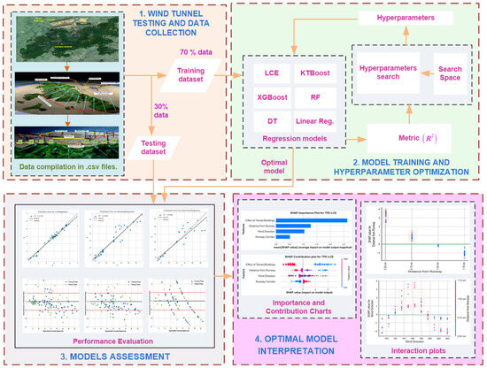
Figure 2.
Framework for the prediction and interpretation of crosswind speed over the airport runway glide path.
The remainder of the article is structured in the following manner: in Section 2, the wind tunnel experiments are presented along with a description of the LCE model, TPE, SHAP, and performance metrics. Section 3 illustrates the computed hyperparameters using the TPE approach, evaluates the performance of the LCE model and other machine learning algorithms, conducted uncertainty analysis and interprets the results using SHAP. Section 4 is dedicated to presenting the conclusions and recommendations.
2. Materials and Methods
2.1. Effect of Wind at Hong Kong International Airport
The geographical location of the Hong Kong International Airport (HKIA) is situated on the subtropical island of Lantau, which is positioned off the southeastern coast of the Chinese mainland, as illustrated in Figure 3 [35]. Multiple experimental and simulation investigations have suggested that the intricate topography and significant contrast between land and sea at HKIA make it vulnerable to the occurrence of harsh weather phenomena. Based on pilot flight reports collected from the Hong Kong International Airport (HKIA), it has been noted that wind shear has impacted roughly 1 in 500 flights since the airport’s opening. Ninety-seven percent of the pilot reports indicated the presence of LLWS ranging from 20 to 25 knots. As per the pilot reports, it was observed that approximately 70% of the wind shear was attributed to terrain-induced factors. In addition to the geographical features, neighboring edifices, as illustrated in Figure 4 [36], are also major sources of low-altitude wind shear, crosswinds and turbulence [37].
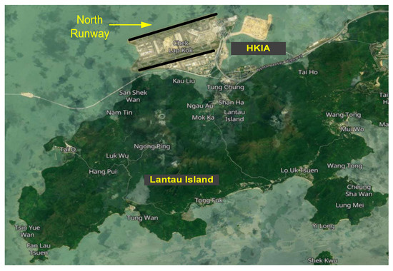
Figure 3.
Hong Kong International Airport near Lantau Island.
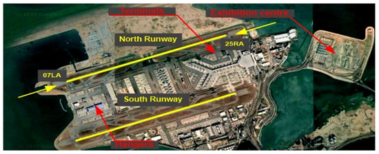
Figure 4.
Buildings near and at Hong Kong International Airport.
2.2. Wind Tunnel Experiments
The current study utilized wind tunnel experiments to assess the crosswind speed over the glide path of the northern runway at Hong Kong International Airport (HKIA) under different inflow wind conditions. The testing area included Lantau Island, Hong Kong International Airport (HKIA), and adjacent structures and terrain, spanning a distance of 27.2 km and having an average elevation of approximately 425.2 m. The experiments were carried out at the TJ-3 ABL wind tunnel, located at the State Key Laboratory for Disaster Reduction in Civil Engineering at Tongji University in Shanghai. The wind tunnel employed in the study was a closed low-velocity wind tunnel featuring a return-type configuration. The dimensions of the testing area were reported as follows: a height of 2 m, a length of 14 m, and a width of 15 m.
The intricate topography, encompassing Lantau Island, adjacent structures, and the northern runway of HKIA, was constructed utilizing a geometric scaling proportion of 1:4000 and a diameter of model as 6.8 m. The process of constructing the terrain model was carried out through a systematic layer-by-layer technique following the contour lines. The material used for this purpose was dense foam with a texture of one inch, which corresponds to a variation in the actual terrain elevation of 40 m, as depicted in Figure 5a. The reduced-scale model’s surface was coated with paint in order to imitate the rough texture of a real mountain. The calculation of the blockage ratio of the wind tunnel was performed through the utilization of Equation (1), which is ratio of the windward or projected area of the test model by the cross-sectional area of the wind tunnel section. The resulting value was determined to be 2.402%, falling below the recommended threshold of 5% for wind tunnel investigations and meeting the necessary criteria for the wind tunnel tests.
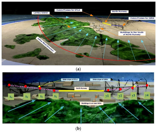
Figure 5.
Scaled model with different inflows.
The wind direction was altered in a methodical manner in 15-degree increments, spanning from 90 to 240 degrees, taking into consideration the established air prevailing trends of easterly to southeasterly winds and the southwest monsoon that is prevalent in Hong Kong, which is depicted in Figure 5b. Eleven distinct types of wind conditions were logged into the data collection system. It was determined that 0 degrees would represent the north wind, 90 degrees would represent the east wind, 180 degrees would represent the south wind, and 270 degrees would represent the west wind.
During the final approach phase, it is standard for an aircraft to maintain a glide path of three degrees over the last three nautical miles prior to landing on the runway. The trajectory of an approaching airplane is depicted by an imaginary slanted line that originates from the end of the runway threshold and has a 3-degree inclination. The empirical data were gathered at multiple locations positioned along the glide slope of the runway 07LA and 25RA. Two distinct sets of eight measurement locations, denoted by (x1, x2, x3, x4) and (y1, y2, y3, y4), were purposefully positioned over the glide paths of runways 07LA and 25RA, correspondingly, as depicted in Figure 5b. The probes were mounted using customized stands, and the installation height was adjusted to ensure alignment with the height of the measurement site. After conducting each operational condition test, the Cobra probes were positioned in the direction of inflow. The determination of the vertical distance of the points of measurement was accomplished through the utilization of a trigonometric expression, as illustrated in Figure 6. The immutability of the glide path set at a 3-degree inclination and the horizontal distances enabled the aforementioned facilitation. The duration of 65.54 s was allotted for sampling each operational circumstance, with a sampling frequency of 1000 Hz.
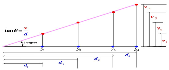
Figure 6.
Computation of vertical distance of measurement points over the glide path.
It is pertinent to mention that none of the tests carried in the wind tunnel simulated a specific inflow profile. Cobra probes were employed to precisely measure the inflow at different elevations, owing to the non-slip nature of the earth/ground. This measure was deemed necessary due to the lack of consistency in the approach flow. The probe registered a minimum wind speed of 2 m/s. The sample experimental outcomes are provided in Table A1.
2.3. Theoretical Overview of Local Cascade Ensemble
This study introduces a novel hybrid ensemble technique, namely Local Cascade Ensemble (LCE), which is trained and tested on the outcomes of wind tunnel experiments. The novel hybrid ensemble technique integrates a boosting–bagging strategy to address the bias-variance trade-off encountered by machine learning algorithms, along with an implicit divide-and-conquer approach for tailoring residuals on particular parts of the data.
The proposed technique amalgamates the advantageous features of the leading tree-based ensemble techniques, namely random forest (RF) [38] and extreme gradient Boosting (XGBoost) [39], and incorporates an additional diversification mechanism to enhance its predictive ability in terms of generalization. Prior to elucidating the process in which LCE integrates these techniques, we shall first introduce the fundamental principles underpinning them, which will subsequently be employed in the explication of LCE. The trade-off between bias and variance characterizes the ability of the machine learning algorithm to extend its performance beyond the confines of the dataset. The presence of systematic errors in the learning algorithm leads to bias, which is a contributing factor to the prediction error. A learning algorithm exhibiting high bias is indicative of its inability to effectively capture the inherent structure of the training set, resulting in under-fitting. The variance is a statistical metric that quantifies the degree of responsiveness of the machine learning algorithm to modifications in the training dataset. A high degree of variance in a machine learning model indicates that it is exhibiting over-fitting behavior by closely tailoring its learning to the data. The aim is to reduce both the bias and variance. The utilization of bagging results in a significant reduction in variance. This technique involves the creation of multiple iterations of a predictor, also known as bootstrap replicates, which are subsequently combined to produce an aggregated predictor. Random forest is the state-of-the-art technique that utilizes bagging and the XGBoost is considered the leading technique that employs boosting. The disparity between bagging and boosting techniques is depicted in Figure 7. The LCE algorithm utilizes a combination of boosting–bagging techniques to effectively address the bias-variance trade-off commonly encountered by machine learning models. Furthermore, it employs a divide-and-conquer methodology to tailor predictor errors to specific segments of the training data. Figure 8 depicts the representation of LCE.
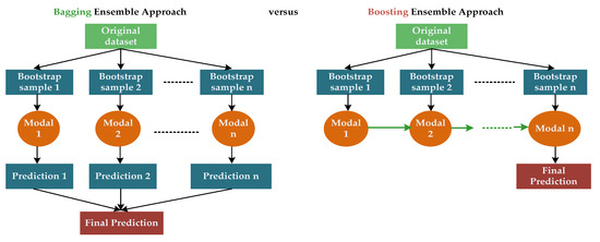
Figure 7.
Working mechanism of bagging and boosting ensemble methods.
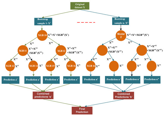
Figure 8.
Working mechanism of LCE.
The LCE approach relies on the principle of cascade generalization, whereby a series of predictors are employed in a sequential manner, with additional attributes being incorporated into the input dataset at each subsequent stage. The novel characteristics are obtained through the utilization of the output produced by a predictor, commonly referred to as a base learner, which provides predictions for a regression problem. The LCE methodology employs a divide-and-conquer approach by locally applying cascade generalization through a decision tree. Additionally, it mitigates bias across the decision tree by utilizing boosting-based predictors as base learners. The base learner utilized in the present study is the state-of-the-art boosting algorithm that has demonstrated a superior performance (XGBoost). Specifically, XGB10 and XGB11 are depicted in Figure 8. During the process of tree growth, the propagation of boosting is achieved by incorporating the output of the base learner at each decision node as additional attributes to the dataset. This can be observed in Figure 8, where XGB10(X1) is added. The predictive performance of the base learner can be evaluated by examining the outputs of the prediction, which indicate its ability to accurately forecast a given sample. At the subsequent tier of the tree structure, the dataset is augmented with additional outputs, which are subsequently utilized by the base learner as a weighting mechanism to prioritize the correction of prior errors or residuals. The utilization of bagging serves to alleviate the over-fitting that arises from the boosted decision tree. Bagging is a technique that aims to reduce variance by generating multiple predictors through the process of random sampling with replacement from the initial dataset. This can be observed in Figure 8, where X1 and X2 are the examples of such predictors. Ultimately, the trees are combined through a basic process of determining the majority vote. The LCE algorithm stores the model generated by the base learner in each node for the purpose of being utilized as a predictor.
2.4. Tree-Structured Parzen Estimator
The efficacy of each machine learning algorithm is dependent on its hyperparameters. They exercise control over the learning model or the foundational structure of the model. In practical application, a universally accepted approach for the selection of hyperparameters is currently non-existent. As a result, hyperparameters are commonly established through a process of trial and error, employing optimization search techniques, or alternatively, are retained with their default settings. The issue of selecting optimal hyperparameters can be addressed in a methodical manner through hyperparameter optimization, which formulates the problem as an optimization task. The aim of this study is to determine a specific set of hyperparameters that can efficiently reduce the disparity between predicted and observed values.
The present study utilized the TPE algorithm to perform hyperparameter tuning. The technique being referred to is a sequential model-based global optimization method that demonstrates proficiency in the identification of hyperparameters for machine learning algorithms. The Parzen window estimators were introduced as a means of addressing the limitations of conventional Bayesian optimization [40,41] in handling categorical and conditional hyperparameters. This development aimed to improve the efficacy of hyperparameter search strategies. The TPE algorithm utilizes Parzen-window density estimation to generate probability density functions in a search space that is hyper-parametric in nature. The formation of the search space can be accomplished through the utilization of a logarithmic uniform or deterministic distribution.
In the iterative process of commencement, an initial distribution is initialized through a random search method that involves the random selection of hyperparameter , where shows the set of hyperparameters, y represents the corresponding outcome of machine learning model via random hyperparameters, and Δ illustrates the required number of iterations. The TPE methodology diverges from traditional Bayesian optimization approaches by employing Parzen window estimators (PWE) as its fundamental building block. The PWE, also referred to as the kernel density estimator, is a widely used empirical approach utilized for the goal of density estimation. The PWE are utilized for the estimation of densities pertaining to both favorable (good) and unfavorable (bad) hyperparameters.
The hyperparameters that were computed are segregated into two sets through the utilization of a quantile threshold value denoted by . It is noteworthy that the selection of this value is arbitrary. The PWE is formulated by normalizing the samples of hyperparameters, whether favorable or unfavorable, with respect to the algorithm’s configuration space, as represented in Equation (2):
where y < y* denotes a higher threshold value than the function value. The equation denoted as Equation (2) can be elucidated as the derivation of two distinct distributions for the hyperparameters. Specifically, one distribution corresponds to the scenario where the function value is below the threshold value, while the other distribution pertains to the situation where the function value exceeds the threshold value. Equation (3) demonstrates the steps for determining the optimal hyperparameter configuration.
The TPE is designed to determine the optimal hyperparameters by utilizing a set of optimal observations and their corresponding distributions, while simultaneously selecting the optimal observations. The TPE process’s comprehensive flowchart is illustrated in Figure 9.
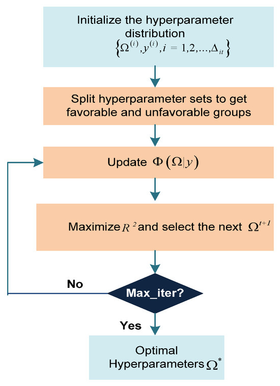
Figure 9.
Working mechanism of TPE (*—optimal value).
2.5. SHAP Interpretation Mechanism
The Shapley additive explanations (SHAP) method, as put forward by Lundberg and Lee [42], is employed for the purpose of interpreting the model’s output. The terminology is derived from Shapley additive explanation, which is an additive explanation model developed by SHAP, drawing inspiration from cooperative game theory [43]. In this model, all the characteristics are considered as “contributors”. In the case of each anticipated sample, the model produces a projected outcome, and the SHAP value represents the assigned value for each characteristic in the sample, as proposed by Shapley [44]. Consider a scenario involving an LCE model, wherein a group denoted as N, consisting of n attributes, is utilized to make predictions for an outcome variable also denoted by N. In the SHAP framework, the allocation of the contributions of each feature (denoted by for attribute i) to the model outcome is determined by their respective marginal contributions. The representation of Shapley values is given by Equation (4), which is based on a set of axioms aimed at ensuring a fair allocation of contributions from every attribute.
2.6. Performance Measures
Various metrics, such as mean absolute error (MAE), mean squared error (MSE), root mean square error (RMSE), and coefficient of determination (R2), can be utilized to assess and contrast the effectiveness of distinct models. The MAE (Equation (5)) is defined as the mean of the absolute values of the prediction errors computed across all instances. Equation (6) is utilized to calculate the MSE, by which the discrepancies between the predicted and actual values is determined. The RMSE is computed as the square root of the difference between the predicted and actual values (Equation (7)). The R2, ranging from 0 to 1, serves as an indicator of the predictive accuracy of a given model (Equation (8)).
where:
—The number of wind tunnel experimental outcomes
—The n-th observed value of crosswind speed from wind tunnel experiment
—The n-th predicted value of crosswind speed from different machine learning model.
—The average value of all crosswind speeds.
3. Result and Discussion
This section has been subdivided into four sub-sections. Section 3.1 presents the optimal hyperparameters of the LCE approach and other machine learning algorithms using the tree-structured Parzen estimator (TPE) approach. The performance of LCE and other machine learning regression models in terms of MAE, MSE, RMSE, and R2 are shown in Section 3.2. Uncertainty analysis is conducted in Section 3.3 and the interpretation by SHAP analysis is illustrated in Section 3.4. It is pertinent to mention that, before the hyperparameter training of the LCE and other competitive machine learning models, the label coding of each factor is performed as shown in Table 1.

Table 1.
Label coding of different parameters.
3.1. Optimal Hyperparameters via TPE
The efficacy of a machine learning model’s predictions and its ability to mitigate over-fitting are heavily influenced by the values assigned to its hyperparameters, particularly the hyperparameters. The present study focused on optimizing the hyperparameters of the LCE model, specifically n_estimators and max_depth, using the TPE approach. The primary goal of this optimization was to improve the performance of the model by increasing the R2 value. The LCE model encompasses a hyperparameter known as n_estimator, which serves to determine the number of boosting iterations that will be performed. The variable “max_depth” denotes the maximum depth that a regression tree can attain. The maximum depth of a tree places a limitation on the quantity of nodes that can exist within it. The magnitude of this hyperparameter governs the manner in which the independent variables interact. Figure 10 illustrates the advancement of the TPE over 50 iterations, utilizing R2 as the metric for both LCE and their competitive machine learning models. The hyperparameters linked to the model were adjusted to maximize the R2 metric, resulting in optimal predictive models. The optimal hyperparameters are illustrated in Table 2.
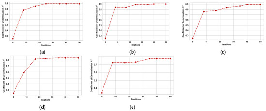
Figure 10.
Progress of TPE for hyperparameter tuning. (a) LCE; (b) XGBoost; (c) KTBoost; (d) RF; and (e) DT.

Table 2.
Optimal hyperparameter values of different machine learning algorithms.
3.2. Prediction Results and Comparative Analysis
In addition to hyperparameter tuning as a strategy for mitigating over-fitting, it is worth mentioning that the dataset was also subjected to shuffling and partitioning, whereby 40% and 50% of the data were, respectively, reserved for testing. The results suggest that the metric values acquired during the testing of the model exhibited stability within a confidence interval of 95%. No abnormal patterns were detected in the metrics when altering the quantity of test data samples. Table 3 illustrates the performance metrics by utilizing both the training and test datasets. The TPE-LCE model exhibited an exceptional performance relative to alternative models, as indicated by its corresponding MAE, MSE, RMSE, and R2 metrics of 0.198, 0.103, 0.319, and 0.953 for the training dataset. The evaluation metrics for the testing data were as follows: the MAE of 0.490, MSE of 0.381, RMSE of 0.617, and R2 value of 0.855. The multivariate linear regression model exhibited poor performance in both the training and testing data, with an MAE of 1.762, MSE of 6.052, RMSE of 2.460, and R2 of 0.629 and with an MAE of 1.593, MSE of 4.359, RMSE of 2.088, and R2 of 0.694, respectively.

Table 3.
Performance evaluation of machine learning models and a statistical model.
The correlation between the results of the experiments and the outcomes estimated by the TPE-LCE model, other machine learning models and a multivariate linear regression model is illustrated in Figure 11 via scatter plots. The results indicate that the TPE-LCE model demonstrated a greater degree of alignment with the 45-degree reference line when compared to alternative models. This was observed through the scatter plot which illustrated the outcomes of crosswind speed estimation from both the training and testing datasets. The clustering pattern of the fitted points of the other models was comparatively more dispersed around the 45-degree baseline, and their predictive precision was inferior to that of the TPE-LCE model.
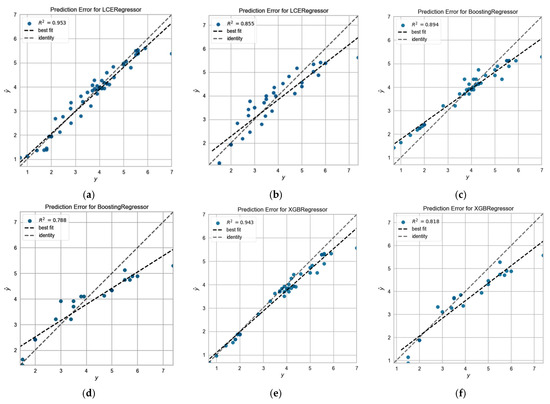
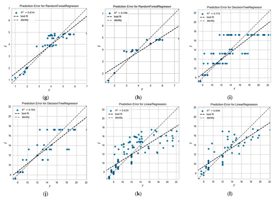
Figure 11.
Plots for the prediction error using both training and testing datasets: (a) TPE-LCE model based on the training dataset; (b) TPE-LCE model based on the testing dataset; (c) TPE-KTBoost model based on the training dataset; (d) TPE-KTBoost model based on the testing data; (e) TPE-XGBoost model based on training data; (f) TPE-XGBoost model based on testing dataset; (g) TPE-RF model based on the training dataset; (h) TPE-RF model based on the testing dataset; (i) TPE-DT model based on the training dataset; (j) TPE-DT model based on the testing dataset; (k) linear regression model based on the training dataset; and (l) linear regression model based on the testing dataset.
3.3. Model Uncertainty Analysis
In order to accurately estimate the crosswind speed along the runway glide path using the TPE-LCE approach, it is imperative to consider the related uncertainties that may arise from the proposed scheme when calculating prediction error. The TPE-LCE model, alternative machine learning models and linear regression model were also compared based on their experimental-to-predicted ratio, as illustrated in Figure 12. In order to establish consistency between the results of the experiments and estimated outcomes, a substantial percentage of the data points (both in the training and testing phases) that are in close proximity (within a range from 0.90 to 1.10) to the unity line serve as a robust indicator of minimal levels of uncertainty. The calculated mean and standard deviation (SD) are also displayed in Table 4. The level of uncertainty in the model decreases as the mean value approaches 1 and the standard deviation decreases. The TPE-LCE model demonstrates a high level of coherence between predicted and experimental values, as evidenced by its mean of 0.988 and standard deviation of 0.078, indicating low levels of uncertainty.
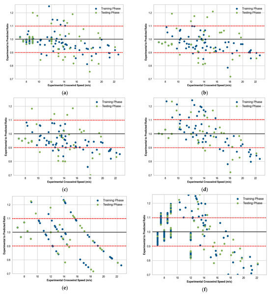
Figure 12.
Uncertainty analysis of the models: (a) experimental-to-predicted ratio for TPE-LCE model; (b) experimental-to-predicted ratio for TPE-KTBoost model; (c) experimental-to-predicted ratio for TPE-XGBoost model; (d) experimental-to-predicted ratio for TPE-RF model; (e) experimental-to-predicted ratio for TPE-DT model; and (f) experimental-to-predicted ratio for linear regression model.

Table 4.
Mean and standard deviation for uncertainty analysis.
3.4. TPE-LCE Model Interpretation by SHAP Analysis
The LCE model was chosen as the optimal fit for the crosswind speed over the glide path based on the R2 value derived from the testing dataset. This section demonstrates the application of SHAP analysis in determining both global and local interpretations, as well as identifying the main effects and interaction effects of factors.
3.4.1. Factor Importance and Contribution
The interpretation of global factors involves the assessment of SHAP factor importance and SHAP factor contribution, which are derived from the prediction results of the TPE-optimized LCE model, as depicted in Figure 13. Figure 13a illustrates the average absolute SHAP value, which represents the average influence on the extent of the model results. The factor labeled “Effect of Terrain/Buildings” exhibited a higher SHAP significance value of 2.52, while the factor denoted “Distance from Runway” had a value of 1.33, and the factor referred to as “Wind Direction” had a value of 1.09. The Bee-swarm plot, depicted in Figure 13b, visually represents the individual contributions of each factor. Factor values are visually represented through a color code, wherein lower factor values are denoted by the color blue, while higher factor values are denoted by the color red. A value of 0 assigned to the “Effect of Terrain/Buildings” factor signifies the non-existence of terrain/buildings and is visually indicated by a blue coloration positioned to the right of a virtual gray line. Non-obstruction serves to depict the increased probability of a higher crosswind speed flowing over the glide path. In a similar vein, it can be observed that the blue and purple dots, which symbolize a shorter distance from the runway, serve as an indicator of a higher crosswind speed. This implies that the probability of crosswind speed is higher in close proximity to the runway.
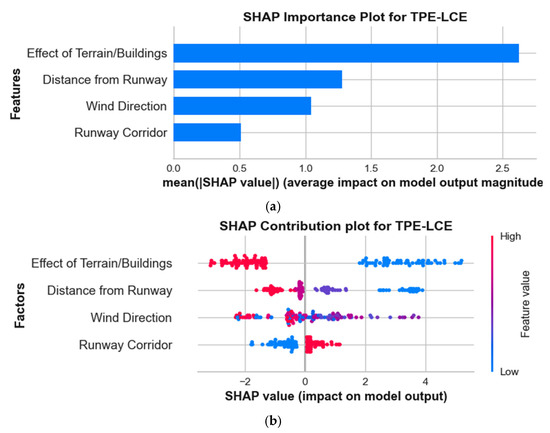
Figure 13.
SHAP interpretation: (a) factors importance graph; and (b) factors bee-swarm graph.
3.4.2. Single Factor Analysis
The SHAP dependence plot, as depicted in Figure 14, serves as a valuable tool for understanding the impact of an individual significant factor on the output of the TPE-optimized LCE model. The horizontal axis denotes the values of the factors, whereas the vertical axis illustrates the SHAP value of each factor. As the narrative progressed, we were able to discern the shifting significance of the factors involved. SHAP values that surpass zero (positioned above the green horizontal line) denote an increased probability of elevated crosswind speed for particular factors. Figure 14a,b depict the influence of two prominent factors, namely “Effect of Terrain/Buildings” and “Distance from Runway,” on the crosswind speed observed over the airport runway glide path. The absence of terrain features and structures, as well as the presence of a crosswind at a distance of 0.75 nautical miles from the threshold of the runway, leads to a SHAP value exceeding 0.00, which signifies an elevated crosswind speed. Furthermore, it can be observed from Figure 14c that wind directions ranging from 129 to 180 degrees are more likely to result in elevated crosswind speeds.
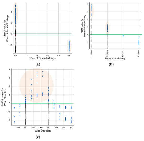
Figure 14.
Single factor analysis: (a) effect of terrain/buildings; (b) effect of distance from runway; and (c) effect of wind direction.
3.4.3. Factor Interaction Analysis
The SHAP interaction plots (Figure 15) are utilized to evaluate the interactions among the factors used to assess the TPE-optimized LCE model in terms of their respective contributions. Figure 15a illustrates a greater intensity of crosswind speed in the proximity of the runway, regardless of the presence or absence of terrain or building influence. The experimental findings suggest that a combination of a shorter distance from the runway threshold and the absence of terrain or buildings is more likely to lead to higher crosswind speeds. There is evidence suggesting that the presence of terrain and buildings near the runway may contribute to increased crosswind speeds. According to Figure 15b, it can be observed that wind directions ranging from 120 to 180 degrees exhibit a higher propensity to generate elevated crosswind speeds. One possible explanation could be attributed to the greater distance of mountainous topography on Lantau Island, which does not impede the airflow in the vicinity of the runway and thereby avoids fluctuations in wind speed.
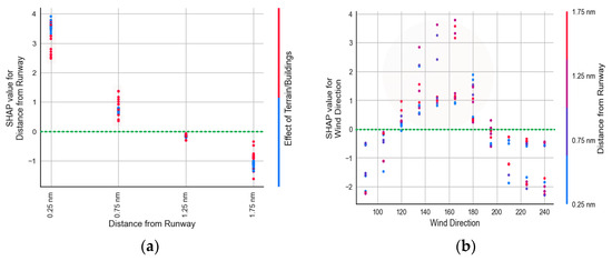
Figure 15.
Interaction analysis of important factors: (a) effect of terrain/buildings and distance from runway; and (b) effect of wind direction and distance from runway.
3.5. Limitation of the Study
The present study employed multiple input variables to estimate the crosswind speed over the runway glide path. However, it is worth noting that future investigations could incorporate additional parameters, such as atmospheric pressure and temperature, to further enhance the accuracy of the estimates. The primary emphasis of the research revolved around the utilization of a machine learning approach in conjunction with the SHAP analysis. Subsequent investigations may consider incorporating various additional methodologies, including deep learning algorithms. The crosswind speed over the runway glide path was a significant parameter of interest in this investigation. Moreover, it is worth considering the inclusion of the turbulence integral length scale as an additional noteworthy wind characteristic for future investigations.
4. Conclusions and Recommendation
This research introduced a novel LCE model that has been optimized through the TPE with the intent of estimating crosswind speeds over the runway glide path. The model’s development was based on the wind tunnel tests. The TPE-LCE model’s predictive capabilities were evaluated in comparison to other contemporary machine learning models including TPE-KTBoost, TPE-XGBoost, TPE-RF, TPE-DT as well as a multivariate linear regression model. The outcomes reveal that the TPE-LCE model exhibited superior predictive capabilities, as evidenced by its lower mean absolute error (MAE) of 0.198, mean squared error (MSE) of 0.103, root mean squared error (RMSE) of 0.319, and higher R2 value of 0.953 for the training dataset. Similarly, the testing dataset also demonstrated a lower MAE of 0.490, MSE of 0.381, RMSE of 0.617, and a higher R2 of 0.855, indicating the model’s robustness in predicting outcomes. The statistical linear regression model exhibited the poorest performance, as evidenced by its MAE of 1.593, MSE of 4.359, RMSE of 2.088, and R2 of 0.694.
The issue of limited interpretability in the TPE-optimized LCE model has been effectively addressed through the utilization of SHAP interpretation strategy. The SHAP analysis, conducted using TPE-optimized LCE predictions, indicated that two factors, namely “Effect of Terrain/Buildings” and “Distance from Runway,” made significant contributions to the likelihood of a high crosswind speed over the runway glide slope/path. The optimal conditions for high crosswind speeds have been identified to be marked by the absence of nearby terrain obstacles or structures, a lesser distance from the runway threshold area, and a prevailing wind direction ranging from 125 to 180 degrees.
The current research utilized multiple input parameters in order to estimate crosswind velocities along the glide path of the northern runway at HKIA. In future research, we may also opt to utilize post hoc interpretive strategies to improve the interpretation efficiency of models, including local interpretable model-agnostic explanations (LIME) and partial dependency analysis (PDA). Furthermore, we would like to emphasize that we have collected pilot reports (PIREPs) from HKIA and acquired weather reports from the Hong Kong Observatory. These additional data sources will provide us with further information regarding temperature and atmospheric pressure. Consequently, our future research will encompass a broader range of factors in order to assess crosswind speeds, thereby yielding a more representative depiction of the actual conditions through wind tunnel experiments and validation by computational fluid dynamics (CFD) simulation.
Author Contributions
Conceptualization, A.K.; Data curation, P.-W.C.; Formal analysis, A.K. and F.C.; Funding acquisition, F.C.; Investigation, F.C. and H.A.; Methodology, A.K. and H.A.; Project administration, J.Z.; Resources, J.Z.; Software, P.-W.C.; Supervision, P.-W.C. and F.C.; Validation, J.Z.; Writing—original draft, A.K.; Writing—review and editing, P.-W.C. and H.A. All authors have read and agreed to the published version of the manuscript.
Funding
The present study received financial support from the National Natural Science Foundation of China (Grant No. 52250410351), the National Foreign Expert Project (Grant No. QN2022133001L), and the Xiaomi Young Talent Program.
Institutional Review Board Statement
Not applicable.
Informed Consent Statement
Not applicable.
Data Availability Statement
Data are unavailable due to privacy.
Acknowledgments
We would also like to express our gratitude to our colleagues at the Hong Kong Observatory of Hong Kong International Airport for their guidance.
Conflicts of Interest
The authors declare no conflict of interest.
Appendix A

Table A1.
Sample data of wind tunnel experiment.
Table A1.
Sample data of wind tunnel experiment.
| Wind Direction | Crosswind Speed | Runway Corridor | Distance from Runway | Effect of Terrain/Buildings |
|---|---|---|---|---|
| 90 | 12.62 | 25RA | At RWY | Considered |
| 105 | 12.73 | 25RA | 3MF | Not considered |
| 120 | 12.91 | 07LA | 3MF | Considered |
| - | - | - | - | - |
| - | - | - | - | - |
| - | - | - | - | - |
| 180 | 21.26 | 25RA | At RWY | Considered |
| 195 | 19.52 | 25RA | At RWY | Considered |
References
- Federal Aviation Administration. Airplane Flying Handbook (FAA-H-8083-3A); Skyhorse Publishing Inc.: New York, NY, USA, 2011.
- Ebbatson, M.; Harris, D.; Jarvis, S. Crosswind landings in general aviation: A modified method of reporting wing information to the pilot. Int. J. Aviat. Psychol. 2007, 17, 353–370. [Google Scholar] [CrossRef]
- Vivaldi, B.E. The Effect of Crosswind and Turbulence in Mental Workload and Pilot Tracking Performance. Master’s Thesis, Embry-Riddle Aeronautical University, Daytona Beach, FL, USA, 2004. [Google Scholar]
- Calle-Alonso, F.; Pérez, C.J.; Ayra, E.S. A Bayesian-network-based approach to risk analysis in runway excursions. J. Navig. 2019, 72, 1121–1139. [Google Scholar] [CrossRef]
- Misagh, K.; Toraldo, E.; Crispino, M. Numerical risk analyses of the impact of meteorological conditions on probability of airport runway excursion accidents. In Computational Science and Its Applications—ICCSA 2020: Proceedings of the 20th International Conference, Cagliari, Italy, 1–4 July 2020; Proceedings, Part I 20; Springer International Publishing: Berlin/Heidelberg, Germany, 2020; pp. 177–190. [Google Scholar]
- Vechtel, D.; Meissner, U.M.; Hahn, K.U. On the use of a steerable main landing gear for crosswind landing assistance. CEAS Aeronaut. J. 2014, 5, 293–303. [Google Scholar] [CrossRef]
- Wu, Y.; Liu, Y. Research on Flight Technique and Hazard Control for Civil Airplane Crosswind Flight Test. In Proceedings of the 2021 International Symposium on Electrical, Electronics and Information Engineering, Seoul, Republic of Korea, 19–21 February 2021; pp. 19–22. [Google Scholar]
- Moren, C.C.R. Teaching landings by the numbers: Quantifying the visual approach and landing. J. Aviat. Aerosp. Educ. Res. 1997, 8, 9. [Google Scholar] [CrossRef][Green Version]
- Smallwood, T. The Airline Training Pilot; Taylor & Francis: Abingdon, UK, 2023. [Google Scholar]
- Niu, J.; Zhang, Y.; Li, R.; Chen, Z.; Yao, H.; Wang, Y. Aerodynamic simulation of effects of one-and two-side windbreak walls on a moving train running on a double track railway line subjected to strong crosswind. J. Wind. Eng. Ind. Aerodyn. 2022, 221, 104912. [Google Scholar] [CrossRef]
- Chen, Z.W.; Liu, T.H.; Yan, C.G.; Yu, M.; Guo, Z.J.; Wang, T.T. Numerical simulation and comparison of the slipstreams of trains with different nose lengths under crosswind. J. Wind. Eng. Ind. Aerodyn. 2019, 190, 256–272. [Google Scholar] [CrossRef]
- Deng, E.; Yue, H.; Ni, Y.Q.; Wang, Y.W.; He, X.H.; Chen, Z.W. A turbulent crosswind simulation method at high-speed railway tunnel entrance: Based on field test and geometric turbulence generator. Phys. Fluids 2023, 35, 015156. [Google Scholar] [CrossRef]
- Charuvisit, S.; Kimura, K.; Fujino, Y. Effects of wind barrier on a vehicle passing in the wake of a bridge tower in cross wind and its response. J. Wind. Eng. Ind. Aerodyn. 2004, 92, 609–639. [Google Scholar] [CrossRef]
- Ding, J.; Yin, W.; Ma, Y. Large eddy simulation and flow field analysis of car on the bridge under turbulent crosswind. Math. Probl. Eng. 2021, 2021, 7579696. [Google Scholar] [CrossRef]
- Lei, L.; Chan, P.W.; Li-Jie, Z.; Hui, M. Numerical simulation of terrain-induced vortex/wave shedding at the Hong Kong International Airport. Meteorol. Z. 2013, 22, 317–327. [Google Scholar] [CrossRef]
- Chen, F.; Peng, H.; Chan, P.W.; Huang, Y.; Hon, K.K. Identification and analysis of terrain-induced low-level wind shear at Hong Kong International Airport based on WRF–LES combining method. Meteorol. Atmos. Phys. 2022, 134, 60. [Google Scholar] [CrossRef]
- Boilley, A.; Mahfouf, J.F. Wind shear over the Nice Côte d’Azur airport: Case studies. Nat. Hazards Earth Syst. Sci. 2013, 13, 2223–2238. [Google Scholar] [CrossRef]
- Rasheed, A.; Sørli, K. CFD analysis of terrain induced turbulence at Kristiansand airport, Kjevik. Aviation 2013, 17, 104–112. [Google Scholar] [CrossRef]
- Zhang, H.; Liu, X.; Wang, Q.; Zhang, J.; He, Z.; Zhang, X.; Li, R.; Zhang, K.; Tang, J.; Wu, S. Low-Level Wind Shear Identification over the glide path at BCIA by the Pulsed Coherent Doppler LiDAR. Atmosphere 2020, 12, 50. [Google Scholar] [CrossRef]
- Tse, K.S. Numerical simulations of terrain-induced turbulent flow around Hong Kong International Airport. Ph.D. Thesis, Hong Kong University of Science and Technology, Hong Kong, China, 2018. [Google Scholar]
- Shimoyama, K.; Nakanomyo, H.; Obayashi, S. Airport terrain-induced turbulence simulations integrated with weather prediction data. Trans. Jpn. Soc. Aeronaut. Space Sci. 2013, 56, 286–292. [Google Scholar] [CrossRef]
- Franchini Longhi, S.N.; Perez Alvarez, J.; Ogueta-Gutiérrez, M.; Gómez-Ortega, O.; Meseguer Garrido, F. Wind tunnel testing on the new control tower of the Fujairah International Airport. In Proceedings of the 15th International Conference on Wind Engineering, Beijing, China, 1–6 September 2019. [Google Scholar]
- Khattak, A.; Chan, P.-W.; Chen, F.; Peng, H. Assessing wind field characteristics along the airport runway glide slope: An explainable boosting machine-assisted wind tunnel study. Sci. Rep. 2023, 13, 10939. [Google Scholar] [CrossRef]
- Chen, F.; Peng, H.; Chan, P.-w.; Zeng, X. Wind tunnel testing of the effect of terrain on the wind characteristics of airport glide paths. J. Wind. Eng. Ind. Aerodyn. 2020, 203, 104253. [Google Scholar] [CrossRef]
- Khattak, A.; Chan, P.W.; Chen, F.; Peng, H. Estimating turbulence intensity over the glide path using wind tunnel experiments combined with interpretable tree-based machine learning algorithms. Build. Environ. 2023, 239, 110385. [Google Scholar] [CrossRef]
- Barua, L.; Zou, B.; Zhou, Y. Machine learning for international freight transportation management: A comprehensive review. Res. Transp. Bus. Manag. 2020, 34, 100453. [Google Scholar] [CrossRef]
- Nama, M.; Nath, A.; Bechra, N.; Bhatia, J.; Tanwar, S.; Chaturvedi, M.; Sadoun, B. Machine learning-based traffic scheduling techniques for intelligent transportation system: Opportunities and challenges. Int. J. Commun. Syst. 2021, 34, e4814. [Google Scholar] [CrossRef]
- Mostafa, K.; Zisis, I.; Moustafa, M.A. Machine learning techniques in structural wind engineering: A State-of-the-Art Review. Appl. Sci. 2022, 12, 5232. [Google Scholar] [CrossRef]
- Meddage, D.P.P.; Ekanayake, I.U.; Weerasuriya, A.U.; Lewangamage, C.S.; Tse, K.T.; Miyanawala, T.P.; Ramanayaka, C.D.E. Explainable Machine Learning (XML) to predict external wind pressure of a low-rise building in urban-like settings. J. Wind. Eng. Ind. Aerodyn. 2022, 226, 105027. [Google Scholar] [CrossRef]
- Weng, Y.; Paal, S.G. Machine learning-based wind pressure prediction of low-rise non-isolated buildings. Eng. Struct. 2022, 258, 114148. [Google Scholar] [CrossRef]
- Lin, P.; Hu, G.; Li, C.; Li, L.; Xiao, Y.; Tse, K.T.; Kwok, K.C. Machine learning-based prediction of crosswind vibrations of rectangular cylinders. J. Wind. Eng. Ind. Aerodyn. 2021, 211, 104549. [Google Scholar] [CrossRef]
- Kim, B.; Yuvaraj, N.; Tse, K.T.; Lee, D.-E.; Hu, G. Pressure pattern recognition in buildings using an unsupervised machine-learning algorithm. J. Wind. Eng. Ind. Aerodyn. 2021, 214, 104629. [Google Scholar] [CrossRef]
- Jiao, Z.; Wang, H.; Xing, J.; Yang, Q.; Zhao, J.; Yang, M.; Zhou, Y. A Local Cascade Ensemble Learning Method for Lithium Ion Battery SOC Estimation under Multi External Factors Considering OCV Hysteresis. In Proceedings of the 2022 Power System and Green Energy Conference (PSGEC), Shanghai, China, 5–27 August 2022; pp. 262–266. [Google Scholar]
- Watanabe, S. Tree-structured Parzen estimator: Understanding its algorithm components and their roles for better empirical performance. arXiv 2023, arXiv:2304.11127. [Google Scholar]
- Hong Kong Lantau Island. Gosur Maps. Available online: https://www.gosur.com/map/hong-kong_islands-district_lantau%20sland/?ll=22.248861393152396,113.92478936610541&z=11.512420070406215&t=satellite (accessed on 2 May 2023).
- Hong Kong International Airport. Gosur Maps. Available online: https://www.gosur.com/map/hong-kong_islands-district_lantau%20sland/?ll=22.30716330676063,113.91088761573155&z=13.198816038941512&t=satellite (accessed on 2 May 2023).
- Chen, F.; Peng, H.; Chan, P.-w.; Zeng, X. Low-level wind effects on the glide paths of the North Runway of HKIA: A wind tunnel study. Build. Environ. 2019, 164, 106337. [Google Scholar] [CrossRef]
- Breiman, L. Random forests. Mach. Learn. 2001, 45, 5–32. [Google Scholar] [CrossRef]
- Chen, T.; Guestrin, C. Xgboost: A scalable tree boosting system. In Proceedings of the 22nd Acm Sigkdd International Conference on Knowledge Discovery and Data Mining, San Francisco, CA, USA, 13–17 August 2016; pp. 785–794. [Google Scholar]
- Snoek, J.; Larochelle, H.; Adams, R.P. Practical bayesian optimization of machine learning algorithms. In Advances in Neural Information Processing Systems, Proceedings of the 25th International Conference on Neural Information Processing Systems, Lake Tahoe, Nevada, 3–6 December 2012; Curran Associates Inc.: LaneRed Hook, NY, USA, 2012; p. 25. [Google Scholar]
- Krause, J.; Perer, A.; Ng, K. Interacting with predictions: Visual inspection of black-box machine learning models. In Proceedings of the 2016 CHI Conference on Human Factors in Computing Systems, San Jose, CA, USA, 7–12 May 2016; pp. 5686–5697. [Google Scholar]
- Lundberg, S.M.; Lee, S.I. A unified approach to interpreting model predictions. In Advances in Neural Information Processing Systems, Proceedings of the 31st International Conference on Neural Information Processing Systems, Long Beach, CA, USA, 4–9 December 2017; Curran Associates Inc.: LaneRed Hook, NY, USA, 2017; p. 30. [Google Scholar]
- Štrumbelj, E.; Kononenko, I. Explaining prediction models and individual predictions with feature contributions. Knowl. Inf. Syst. 2014, 41, 647–665. [Google Scholar] [CrossRef]
- Shapley, L.S. A Value for N-Person Games; Defense Technical Information Center: Fort Belvoir, VA, USA, 1953; Volume 2, pp. 307–317.
Disclaimer/Publisher’s Note: The statements, opinions and data contained in all publications are solely those of the individual author(s) and contributor(s) and not of MDPI and/or the editor(s). MDPI and/or the editor(s) disclaim responsibility for any injury to people or property resulting from any ideas, methods, instructions or products referred to in the content. |
© 2023 by the authors. Licensee MDPI, Basel, Switzerland. This article is an open access article distributed under the terms and conditions of the Creative Commons Attribution (CC BY) license (https://creativecommons.org/licenses/by/4.0/).