Abstract
In March 2022, a new wave of COVID-19 outbreak occurred in Shanghai due to the widespread transmission of the Omicron variant. A two-month citywide lockdown was implemented from April 1st to May 31st, adopting measures such as zone-based classification and grid management. This unique social event provided an “ideal air quality experiment” for pollution research. The rapid reduction in economic activities during the lockdown had many positive impacts on the environment, leading to overall improvements in air quality. Particularly, the concentration of NOx, one of the precursors to O3, significantly decreased. However, O3, as a typical secondary pollutant, showed a noticeable increase. This study uses the WRF-CAMx-OSAT air quality model method to analyze the source of O3 pollution in Shanghai from April to May 2022. The impact of O3 precursor control, sector sources, and regional contributions on the formation of O3 pollution in Shanghai is analyzed in depth. During the pandemic lockdown period, it was found that, in Shanghai, the overall O3 levels were controlled by VOCs (Volatile Organic Compounds), and controlling VOCs proved to be an effective measure in reducing O3 concentrations in Shanghai. Compared with the same period in 2021, the proportion of road traffic sources contributing to ozone concentration has significantly decreased from 70.61% to 64.3%, but they are still the largest contributor. The contribution of industrial emissions to the ozone concentration has significantly risen from 20.71% to 26.36%, making them still the second largest contributor. Industrial and traffic sources are emission sources that require particular attention. The contribution ratio of local sources to external transport is about 7:3, which is higher than the ratio of local sources to external transport in the same period of 2021, which is about 6:4. The local ozone is the main source of ozone concentration in Shanghai, and controlling local source emissions is the key to controlling ozone concentration in the Shanghai area. When excluding the impact of long-range transport, the main areas contributing to O3 formation from local sources are Baoshan District, Jiading District, Qingpu District, and Chongming District, accounting for approximately 41.12% of the total absolute contribution. Different source regions exhibit significant spatial variations in their contributions to the ozone concentration. Through these studies, we aim to provide scientific support and control suggestions for the precise prevention and control of O3 pollution in Shanghai.
1. Introduction
Since the outbreak of the COVID-19 pandemic in early 2020, countries around the world have implemented control measures in affected areas to curb the spread of the virus. These measures include the closure of public places and restrictions on human mobility to reduce unnecessary human activities. Studies have shown that COVID-19 pandemic control measures have had a significant impact on reducing emissions in the atmosphere, to the maximum extent possible [1].
The rapid reduction in economic and social activities during the lockdown period has had some positive impacts on the environment, with a general improvement in air quality. Specifically, the concentration of NOx, one of the precursors to O3, significantly decreased; however, O3, as a typical secondary pollutant, exhibited a significant increase in most urban areas, especially in densely populated metropolitan regions with higher levels of human activity [2]. By comparing the PM2.5 and O3 monitoring data in Shanghai from 1 April to 31 May 2022, with the same period in 2021, it was found that the average concentration of PM2.5 in Shanghai decreased by 26.8% during this period. However, the maximum daily 8 h average (MDA8) concentration of O3 increased by 14.5%. This is consistent with previous research results, which showed a general improvement in air quality during the lockdown period, while the ozone concentration exhibited an increasing trend [2]. (Data source: Air Quality Online Monitoring and Analysis Platform https://www.aqistudy.cn, (accessed on 6 May 2023)).
The formation of O3 is a complex process that involves atmospheric chemical reactions and the interaction of various factors. The primary pathway for ozone formation is through photochemical reactions. Under the influence of sunlight, NOx and VOCs undergo photolysis reactions, producing free radicals such as nitrogen oxide radicals (NO3) and hydroxyl radicals (HO). These radicals further react with oxygen (O2) to generate ozone. The formation of ozone involves complex factors such as photochemical reactions, NOx cycling, contributions from VOCs, meteorological conditions, and regional transport. Ground-level ozone is considered one of the most significant air pollutants that adversely affects human health (such as the respiratory and cardiovascular systems), vegetation, and materials [3,4].
At the urban scale, the anthropogenic emissions of VOCs and NOx are heavily influenced by human activities. Urban NOx emissions primarily come from fossil fuel combustion, while VOCs have diverse anthropogenic sources. The formation of O3 depends on the ratio of VOCs to NOx [5]. Research by Zeng et al. [6] indicated that, after strict lockdown measures were implemented in Wuhan, the reduction in NOx emissions exceeded that of VOC emissions, resulting in an increased VOCs–NOx ratio and consequently increasing O3 production. Sicard et al. [7] studied the air quality during the COVID-19 lockdown in Rome and Turin (Italy), Nice (France), Valencia (Spain), and Wuhan (China). They suggested that the increase in O3 was due to a significant reduction in local nitrogen oxide emissions, primarily NO emissions, resulting in weakened titration processes. During the lockdown period, the increase in emissions of carbon monoxide and ozone precursors such as volatile organic compounds from sources like household activities (e.g., cleaning, fireplace use) and outdoor activities (e.g., barbecues, biomass burning) may also be contributing factors to the observed rise in ozone levels [8]. Tanvir et al. [9] used a highly precise Multi-Axis Differential Optical Absorption Spectroscopy (MAX-DOAS) instrument to study the impact of reduced human activities during the 2020 control measures on air quality in Shanghai. They found that the concentration of ozone was not influenced by the control measures and continued to steadily increase during the study period, coinciding with the enhanced solar radiation in late winter and early spring. Huang et al. [10] found that the reduction in NOx emissions from transportation during the COVID-19 pandemic in eastern China increased O3 concentrations and facilitated nighttime NO3 radical formation, leading to an elevated aerosol oxidative capacity (AOC) and increased secondary organic aerosols (SOA). Wang et al. [11] pointed out, based on the simulation results of WRF-Chem, that during the COVID-19 lockdown period from 1 January to 18 April 2020, in China, the atmospheric oxidative capacity significantly increased. The levels of oxidants increased (up to +25%), particularly in southern Jiangsu, Shanghai, and northern Zhejiang, ultimately leading to an increase in O3.
Air quality modeling is an important technical tool for studying O3 and can be used for O3 sensitivity analysis, the identification of key controlling factors, and source apportionment. Among the air quality monitoring methods, the CAMx-OSAT (Comprehensive Air Quality Model with Extensions-Ozone Source Apportionment Technology), based on a three-dimensional Eulerian chemical transport model, provides source apportionment or source contribution capabilities. In a single-model run, it can assess the temporal and spatial contributions of multiple source regions, categories, and pollutant types to levels of O3 and particulate matter. OSAT is based on an improved O3 source apportionment method, which estimates the contributions of emissions from different regions to O3 concentrations. This method categorizes regions into NOx control zones, VOC control zones, and transition zones, attributing O3 formation at each time step to the precursors NOx and VOCs, which are then labeled as O3N and O3V. In the model, tracers are used to estimate the contributions of different regions to O3N and O3V levels, and these contributions are used to determine the regional contributions to O3 concentrations. This approach calculates source region contributions to the target region, considering both the transport of O3 precursors generated in the source region to the target region and the generation of O3 precursors in the target region itself. This allows for the comprehensive simulation and assessment of atmospheric pollutants at various scales, including the urban and regional levels. Currently, research on O3 source apportionment in China mainly focuses on heavily polluted and economically developed regions such as the Beijing-Tianjin-Hebei area [12,13,14], the Yangtze River Delta [15,16,17,18], and the Pearl River Delta [19,20,21,22].
From 1 April to 31 May 2022, Shanghai implemented a two-month citywide lockdown, adopting measures such as zonal classification and grid management. This special period greatly reduced economic and social activities to nearly the lowest level, providing an “ideal air quality experiment” for pollution research. This study employed the WRF-CAMx-OSAT air quality modeling approach to investigate the spatiotemporal distribution characteristics of O3 pollution in Shanghai during April and May 2022. OSAT was employed to assess the impacts of various sectors and regional contributions on O3 pollution formation in Shanghai. The aim was to identify sectors and regions with significant influence on O3 concentrations. Through this research, this study aimed to reveal the spatiotemporal distribution of O3 concentrations during the lockdown period in Shanghai, the effects on the ozone formation mechanisms in Shanghai, the substantial emission reductions resulting from the lockdown and their impact on air quality in Shanghai, and the differences in contributions to O3 concentrations between the lockdown and normal conditions. The goal was to provide scientific support and control recommendations for the precise prevention and treatment of O3 pollution in Shanghai based on these findings.
2. Materials and Methods
2.1. WRF-CAMx-OSAT Simulation Method
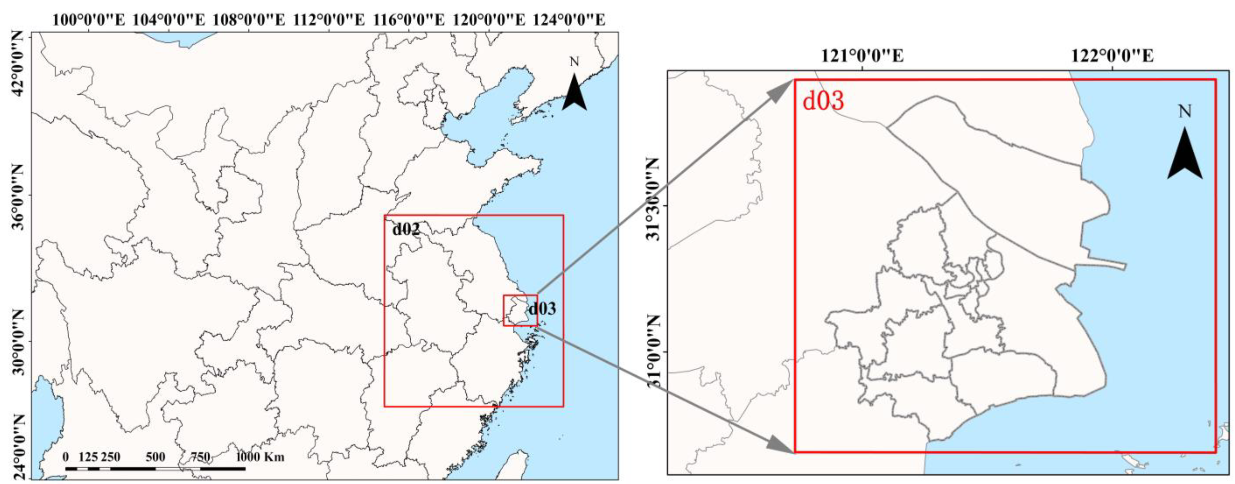
The WRF-CAMx-OSAT simulation method was employed, using the WRF 3.9.1 (Weather Research and Forecasting) model to provide meteorological fields for the CAMx model. The parameterization schemes for WRF and CAMx can be found in Table S1. In Figure 1, the WRF simulation adopted a three-level nested domain with grid resolutions of 9 km, 3 km, and 1 km, respectively. The center point of the model projection was set at (31.9° N, 118.51° E). The first domain covered the East China region, the second domain covered the Yangtze River Delta region, and the third domain focused on the Shanghai area. Localized settings for the main parameters of the WRF model were applied to match the climatic background of Shanghai. The initial and boundary conditions for the WRF model were obtained from the Global Final Analysis data, provided by the National Centers for Environmental Prediction (NCEP) in the United States. The data were available at a horizontal resolution of 1 × 1 and were retrieved from the NCEP FNL Operational Model Global Tropospheric Analyses dataset, continuing from July 1999 (https://rda.ucar.edu/, accessed on 14 April 2023).
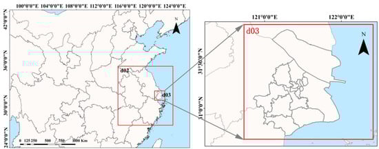
Figure 1.
WRF model simulation domain.
This study utilizes CAMx version 6.5 for comprehensive modeling. CAMx, based on the “one atmosphere” framework, simulates pollutant emissions, dispersion, chemical reactions, and atmospheric removal processes by solving the physical and chemical transformation equations for each pollutant in each grid cell at various scales, including the urban and regional scales [23,24]. The OSAT (Ozone Source Apportionment Technology) is a source apportionment technique integrated into the CAMx numerical model. OSAT calculates the contributions of regional and sectoral emission sources to the formation (or emission) and removal of O3 and its precursors using a tracing method. It provides clear information about the regional and sectoral sources’ contributions to O3 and its precursors for selected time periods and receptor locations. CAMx-OSAT uses the CB05 chemical mechanism, SOAP/CF aerosol scheme, Wesely resistance model for dry deposition, Seinfeld and Pandis scheme for wet deposition, and boundary and initial conditions from the real-time output of the MOZART-4 global model. CAMx has a two-layer nested grid configuration, with the same resolution and grid center points as the second and third layers of WRF. To minimize the impact of boundary fields on air quality simulations, the CAMx grid is slightly smaller than the WRF grid. In the vertical direction, 28 pressure levels are set with increasing spacing from near the surface. The atmospheric O3 column data required for the photolysis rate parameter in the model are obtained from the daily O3 observations provided by NASA Ozone Watch (https://ozonewatch.gsfc.nasa.gov/data/omi/, accessed on 24 April 2023).
In the source apportionment analysis, the second nested layer is divided into 9 regions: Central Urban Area (Huangpu District, Jing’an District, Xuhui District, Changning District, Yangpu District, Hongkou District, Putuo District), Minhang District, Baoshan District and Jiading District, Chongming District, Pudong New Area, Jinshan District and Fengxian District, Songjiang District, Qingpu District, and Other Areas (areas outside Shanghai). The analysis considers four pollution sources: natural sources, industrial sources (including industrial sources and power sources), transportation sources, and other sources (including agricultural sources and residential sources). These sources are further categorized into 36 groups to assess their contributions to O3 formation.
2.2. Emission Inventory during the Lockdown Period
In this study, the term “COVID-19 lockdown period” refers to the period from 1 April 2022 to 31 May 2022, in the Shanghai region. This study utilizes the 2017 Multi-resolution Emission Inventory for China (MEIC), developed by Tsinghua University, as a bottom-up emission inventory model, and the 2017 anthropogenic emission inventory for the Yangtze River Delta compiled by the Shanghai Academy of Environmental Sciences in 2017 as the baseline. Assuming that, during the pandemic period (from the beginning of 2020 to 2022), the industrial structure and its distribution in Shanghai, as well as the overall level of air pollution control, remained relatively unchanged from the baseline emission scenario, the variation in emissions during the 2022 lockdown period (April and May) can be attributed to the changes in socio-economic activities caused by the lockdown measures. The changes in emissions during the Shanghai lockdown in April and May 2022 are calculated by adjusting the “baseline scenario” based on the variations in socio-economic activities. In this study, the period from 1 April 2022 to 31 May 2022 was used as the non-lockdown period, and the emissions inventory during this period was taken from the “baseline scenario” for comparison with the lockdown period. Therefore, the changes in pollutant emissions are only related to changes in activity levels. The estimation of emission reductions needs to be conducted based on the changes in activity levels to establish an emission inventory for the lockdown period.
In Equation (1), represents the emissions of pollutant k from emission source j in region i during the lockdown of the COVID-19 pandemic. represents the ratio of the activity levels between the lockdown period and the corresponding period in 2021 without lockdown for emission source j in region i.
The biogenic emission data are sourced from the global vegetation emission inventory published on the HEMCO website with a resolution of 0.25 × 0.3125 (http://wiki.seas.harvard.edu/geos-chem/index.php/FlexGrid, accessed on 5 April 2023). The emission data for the first layer of industrial sources (including industrial and power sources), transportation sources, and other sources (including agricultural and residential sources) are obtained from the MEIC inventory (http://meicmodel.org/, accessed on 5 April 2023). The resolution for all sources except shipping sources is 0.25°, while the resolution for shipping sources is 0.5°. The second and third layers of industrial sources, transportation sources, and other sources are provided by the Shanghai Environmental Science and Engineering Institute (ESEI) in the form of a human-made emission inventory for the Yangtze River Delta region, with a resolution of 4 km. Following the principle of emission conservation, the emission data from the MEIC inventory and the ESEI inventory are interpolated to match the grid and resolution of each nested layer in CAMx using bilinear interpolation. Additionally, the emission inventory for Shanghai is adjusted based on survey data to account for emission reductions.
2.3. Social and Economic Statistical Data during the Lockdown Period
To estimate the emission reductions resulting from the COVID-19 lockdown, we selected 32 near-real-time dynamic economic and industrial activity level data (Table S2) to estimate the emissions in Shanghai for April and May 2022. The activity level data for the thermal power sector were obtained from the monthly statistical data of the National Bureau of Statistics (https://data.stats.gov.cn/, accessed on 5 November 2023), showing a year-on-year decrease in electricity generation of 41.1% and 41.4% for April and May 2022, respectively. Since all power generation in Shanghai is from thermal power plants, we assume that the reduction in electricity generation represents the impact of the COVID-19 lockdown on atmospheric pollutant emissions from the power sector [10]. Therefore, the emissions from the power sector in April and May 2022 were estimated to decrease by 41.1% and 41.4% compared to the same period in 2021.
The same approach was applied to the industrial sector. The production volume data for the selected 26 industrial sectors, such as edible vegetable oil, ethylene, steel, cement, etc., were obtained from the Shanghai Statistics Bureau (https://tjj.sh.gov.cn/, accessed on 5 November 2023) and the National Bureau of Statistics (https://data.stats.gov.cn/, accessed on 6 November 2023) monthly statistical data. Assuming that the reduction in production volume of the major industrial sectors represents the impact of the COVID-19 lockdown on atmospheric pollutant emissions from the industrial sector, the industrial emissions in Shanghai for April and May 2022 were estimated to decrease by 59.4% and 22.5% compared to the same period.
As for the residential sector, emissions from boilers and stove commercial use in the Shanghai area have been considered negligible following the implementation of the lockdown measures, while emissions from household cooking are assumed to be unaffected.
For the transportation sector, the activity level data for the turnover of goods and passengers on highways, railways, and waterways were obtained from the Ministry of Transport of the People’s Republic of China (https://www.mot.gov.cn/, accessed on 6 November 2023). It is assumed that the reduction rate in the turnover of goods and passengers is the impact of COVID-19 lockdowns on emissions of pollutants in the transportation sector. According to transportation index data, the turnover of goods and passengers in April and May 2022 decreased by 45.1% and 41.8% compared to 2021. During the COVID-19 lockdown period, the activity level of non-road mobile machinery is assumed to be close to zero. Therefore, the road emissions in April and May 2022 decreased by 45.1% and 41.8% compared to 2021.
3. Results and Discussion
3.1. Model Validation
3.1.1. Evaluation Methods
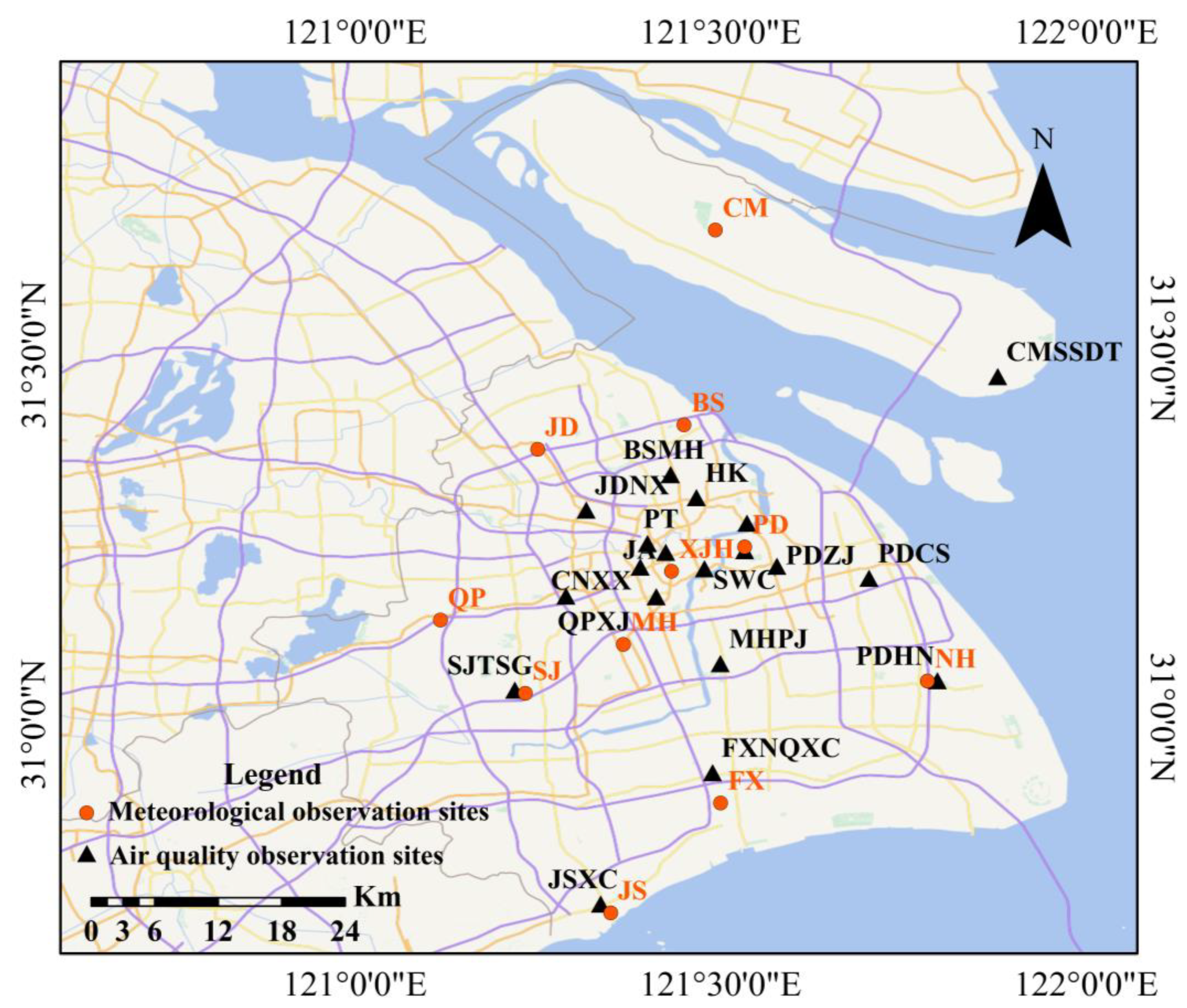
Comparisons between the simulated results of the WRF-CAMx model and the observed data were conducted to validate the accuracy of the simulation in this study. For the simulation of meteorological fields, hourly observed data of various meteorological elements from 11 stations within the Shanghai area, including Baoshan (BS), Chongming (CM), Fengxian (FX), Jiading (JD), Jinshan (JS), Minhang (MH), Nanhui (NH), Pudong (PD), Qingpu (QP), Songjiang (SJ), and Xujiahui (XJH), were used for validation. The observed data covered the period from 1 April 2022 to 31 May 2022 (source: https://xihe-energy.com/, accessed on 12 May 2023). For the pollution field simulation, the simulated results for conventional pollutants (PM2.5, O3, NO2, SO2) were validated using hourly average monitoring data from 19 national monitoring stations in Shanghai from 2 April 2022 to 30 April 2022 (source: https://www.aqistudy.cn/, accessed on 6 May 2023). The selected monitoring stations included Baoshan Miaohang (BSMH), Fengxian Nanqiao New Town (FXNQXC), Hongkou (HK), Jiading Nanxiang (JDNX), Jinshan Xincheng (JSXC), Minhang Pujiang (MHPJ), Pudong Huinan (PDHN), Jing’an (JA), Pudong Chuansha (PDCS), Pudong New Area (PDXQ), Pudong Zhangjiang (PDZJ), Putuo (PT), Shiwuchang (SWC), Xuhui Shangshida (XHSSD), Yangpu Sipiao (YPSP), Qingpu Xujing (QPXJ), Changning Xianxia (CNXX), Chongming Shangshi Dongtan (CMSSDT), and Songjiang Library (SJTSG). The distribution of the meteorological and pollutant monitoring stations used for validation in this study is shown in Figure 2.
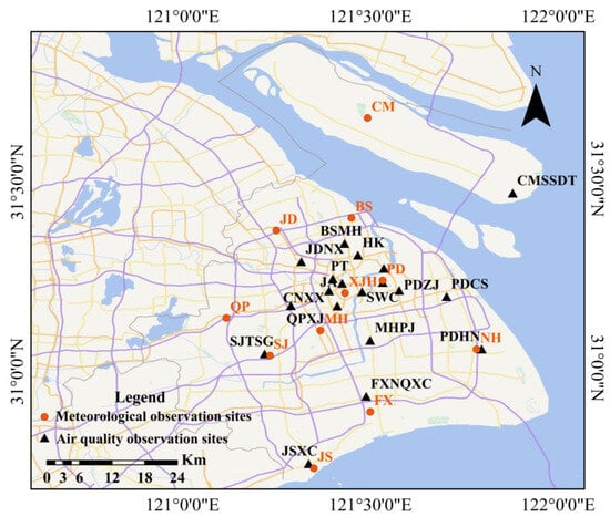
Figure 2.
Distribution of meteorological and air quality observation stations (Source of the base map: http://xdc.at/map/wmts/, accessed on 18 May 2023).
Using the observed data from meteorological stations, the model performance evaluation for four meteorological variables, namely temperature, relative humidity, wind speed, and wind direction, was conducted following the evaluation criteria recommended by the U.S. Environmental Protection Agency (EPA). The selected evaluation parameters include mean bias, root mean squared error (RMSE), and correlation coefficient (COR). For vector variables (wind direction), only two parameters, MB and RMSE, were considered. The expressions for the selected evaluation parameters are as follows:
In the equations, represents the observed value, represents the simulated value, N represents the sample size, and represent the mean values of the observed and simulated results, respectively.
3.1.2. Evaluation of Meteorological Field Simulation
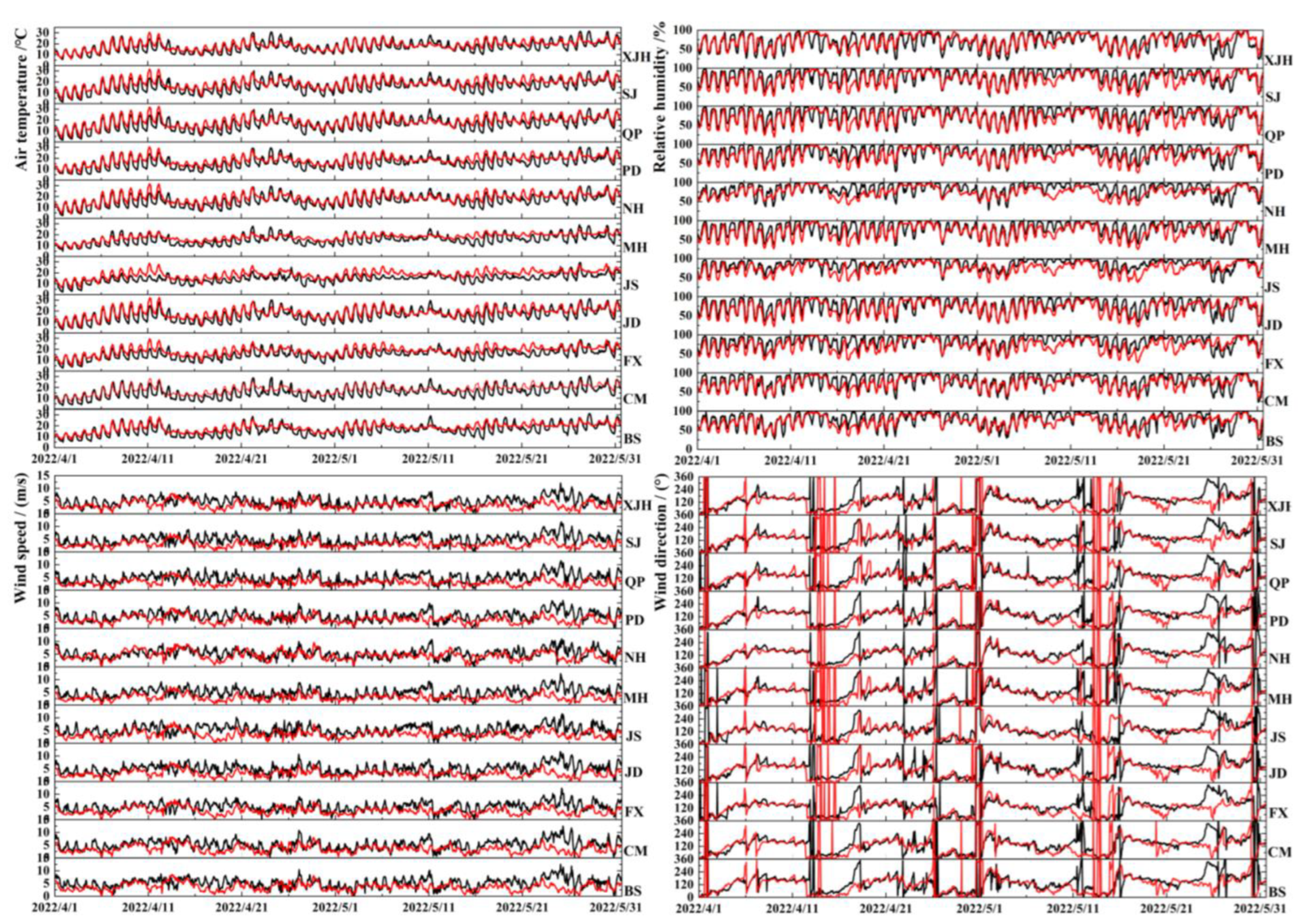
A comparison of the simulated and observed time series for temperature, relative humidity, wind speed, and wind direction in April and May 2022 was conducted. The time series comparison plots for temperature, relative humidity, wind speed and wind direction are presented in Figure 3. The performance of the meteorological variables is summarized in Table 1.
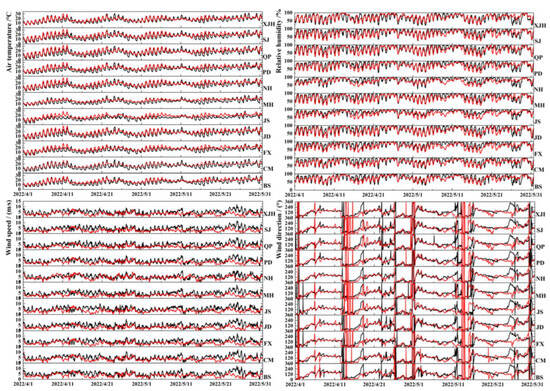
Figure 3.
Time series comparison of temperature, relative humidity, and wind speed between simulated and observed values at various meteorological observation stations. (Red represents observed values and black represents simulated values).

Table 1.
Statistics of meteorological elements simulation results. (From 1 April 2022 to 31 May 2022).
As shown in Figure 3, the simulated temperature values at the 11 stations in Shanghai are in good agreement with the observed values and exhibit significant diurnal variation. The simulated temperatures reach their peak in the afternoon and reach their lowest point from the late night to the early morning, showing good consistency with the observed values. However, it can also be observed that the model’s performance in simulating temperature is poorer during the nighttime, with a noticeable underestimation. Regarding the simulation of relative humidity, the simulated values also show good consistency with the observed values. The diurnal variation in the relative humidity exhibits a trough in the afternoon and a peak during the nighttime. As for the wind speed simulation, although there is considerable variability in the diurnal pattern, the model performs well in simulating wind speed at the 11 stations, showing good agreement with the observed values. However, there are some instances where the model tends to overestimate wind speed on certain dates and times. For wind direction simulation, the model can generally capture wind direction changes at different locations.
As shown in Table 1, overall, the model tends to underestimate the temperature in its simulation. Among the 11 stations in Shanghai, except for the Jiading station, temperatures are underestimated, with the temperature mean bias ranging from −0.10 °C to 0.11 °C. The model shows a relatively small root mean squared error (RMSE) for temperature simulation at the 11 stations, and the simulated temperatures exhibit a high correlation (COR) with the observed temperatures, with all COR values reaching 0.78 or higher. For the simulation of the relative humidity, the MB ranges from −2.42% to 10.35%, the RMSE ranges from 14.14% to 16.45%, and the COR is relatively high, all above 0.65. Typically, the model exhibits significant uncertainties in simulating near-surface wind speed and wind direction. In this study, for the wind speed simulation, all 11 stations show a slight overestimation of the wind speed. The wind speed MB ranges from 0.45 m/s to 1.58 m/s, and the RMSE ranges from 2.19 m/s to 2.64 m/s. The COR values for the wind speed simulation are also relatively high, all above 0.54. For the wind direction simulation, the MB ranges from 4.82° to 15.05° at the 11 stations, and the RMSE ranges from 58.44° to 73.10°.
The comparison and analysis of the observed data and simulation results indicate that, during the simulation period of this study, the model performs well in simulating various meteorological elements. It can effectively reproduce the temperature, humidity, and wind fields, as well as local meteorological processes during the simulation period, providing reliable meteorological background fields for the simulation of pollutants in the region.
3.1.3. Simulation Verification of Pollution Field
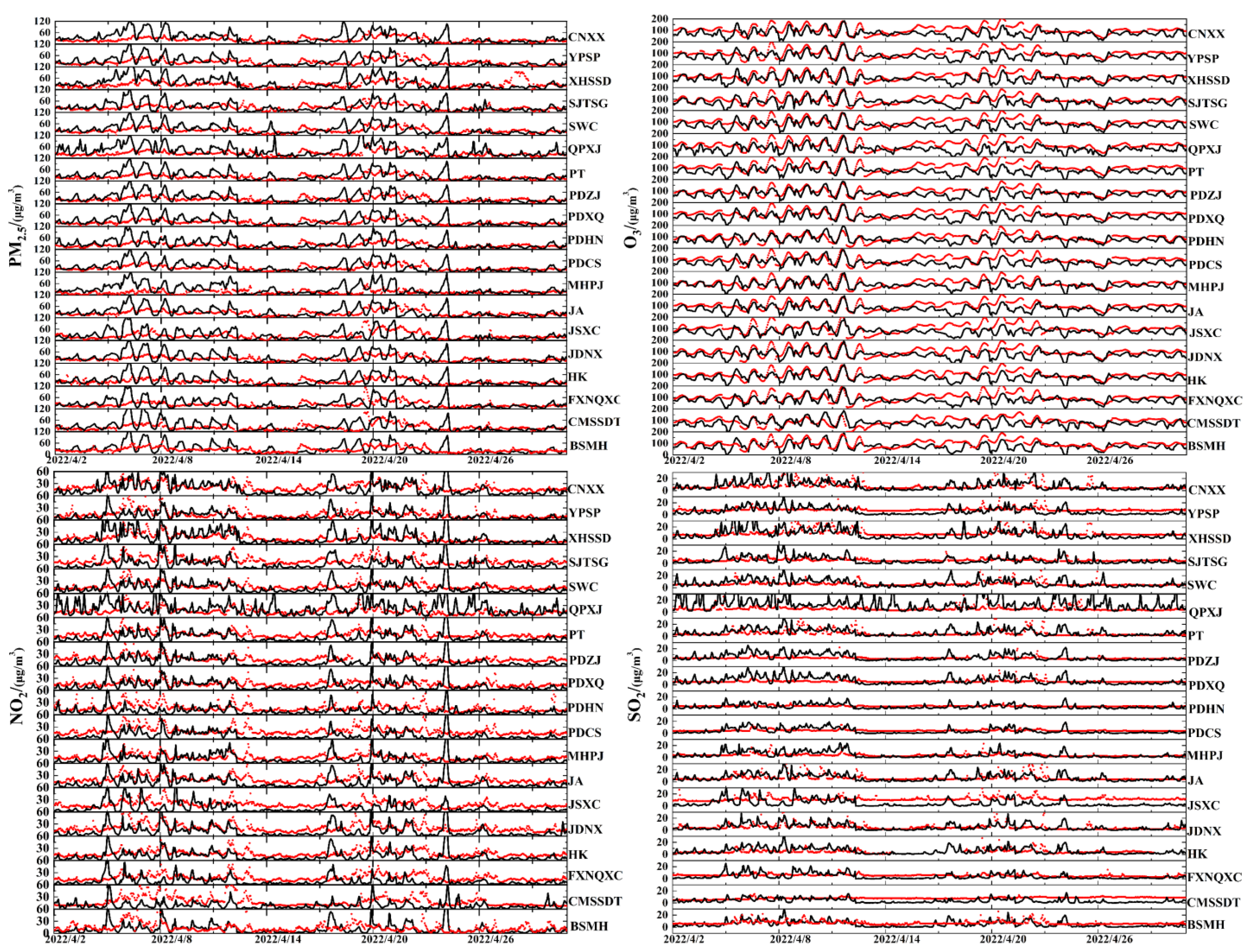
As for the verification of the pollution field, similar to the evaluation of the meteorological field simulation results, the concentration of pollutants was evaluated using indicators such as MB, RMSE, and COR. Hourly monitoring data of conventional pollutants (PM2.5, O3, NO2, SO2) from the 19 national monitoring stations in Shanghai were selected, and hourly average values were compared with the simulation results for validation. The time series of the simulation and observed values are shown in Figure 4. The statistical results of the simulation effectiveness for major pollutant concentrations in different seasons are presented in Table 2.
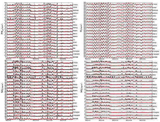
Figure 4.
Time series of PM2.5, O3, NO2, and SO2 between simulated and measured values at observation stations (red represents observed values and black represents simulated values).
Table 2.
Statistics of pollutants simulation results (from 1 April 2022 to 30 April 2022).
From Figure 4, it can be observed that, overall, the CAMx model can reasonably simulate the pollution levels of and temporal variations in major pollutants in Shanghai. Regarding PM2.5 simulation, there are instances where the model overestimates the PM2.5 concentrations. As for O3, typically, O3 concentrations peak in the afternoon and reach a minimum in the early morning and nighttime. The model exhibits good performance in simulating the daily variation in O3 concentrations. However, the O3 concentrations in Shanghai are slightly underestimated, which can be attributed to the uncertainty in emission inventories, resulting in deviations in the simulation results [25,26]. The model shows good performance in simulating SO2 and NO2, and the observed and simulated values of the SO2 and NO2 concentrations are in good agreement across different regions.
From the statistical results, it can be seen that the correlation coefficients between the simulated results of conventional pollutants in Shanghai and the monitoring data are above 0.50, and the MB values for each pollutant are within ±27 μg/m3. It can be concluded that the simulation performance and deviation levels of WRF-CAMx in the chemical field are comparable to other research findings [27], indicating that the simulation results can be used for further source apportionment of ozone.
3.2. Changes and Characteristics of the Emission Inventory during the Lockdown Peri
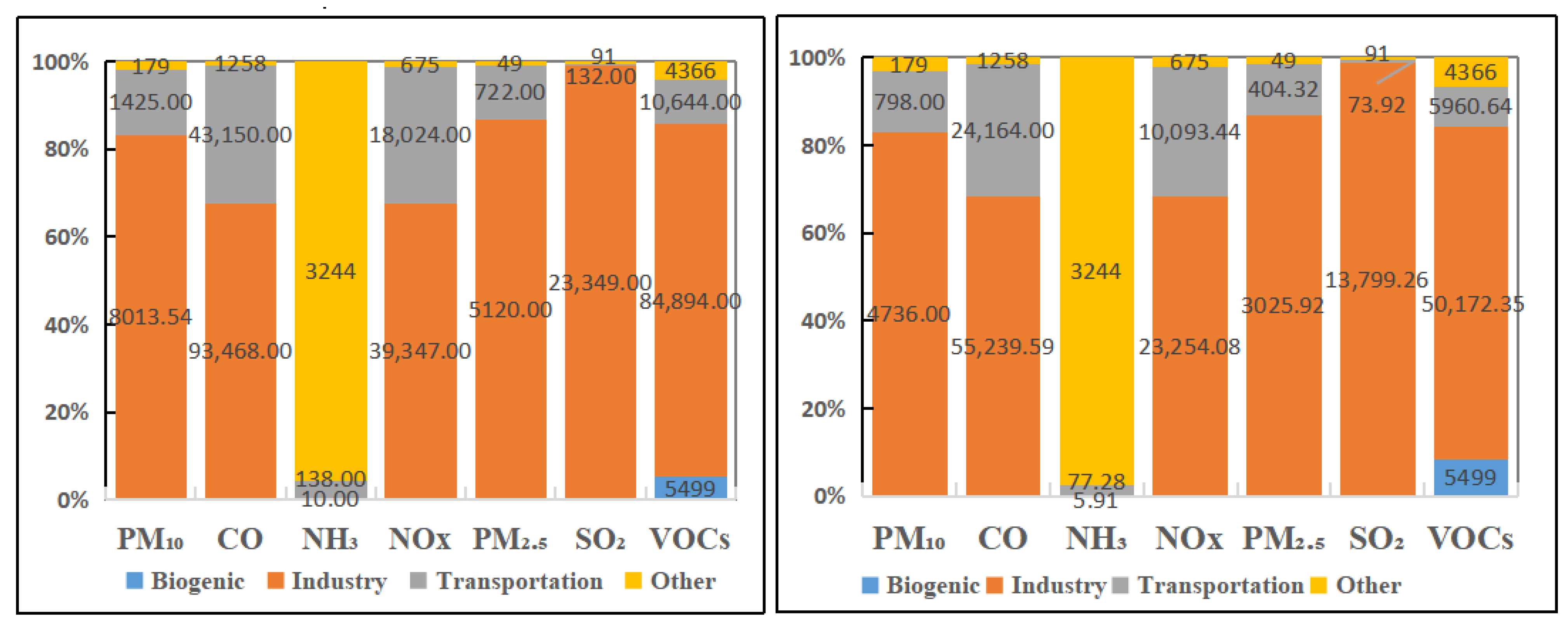
Due to the inherent uncontrollable nature of biogenic emissions, this study focuses only on the anthropogenic emission changes resulting from the pandemic lockdown measures. The biogenic emissions of VOCs remain unchanged at their original levels. In April–May 2021, the total anthropogenic emissions of major air pollutants (PM10, CO, NH3, NOx, PM2.5, SO2, VOCs) in Shanghai were as follows: 9.62 × 10³, 1.38 × 10⁵, 3.39 × 10³, 5.81 × 10⁴, 5.89 × 10³, 2.36 × 10⁴, and 9.99 × 10⁴ (tons). In April–May 2022, the total anthropogenic emissions of major air pollutants (PM10, CO, NH3, NOx, PM2.5, SO2, VOCs) were as follows: 5.71 × 10³, 8.07 × 10⁴, 3.33 × 10³, 3.40 × 10⁴, 3.48 × 10³, 1.40 × 10⁴, and 6.05 × 10⁴ (tons). The reduction percentages for each pollutant are as follows: 40.64% (PM10), 41.52% (CO), 1.77% (NH3), 41.48% (NOx), 40.92% (PM2.5), 40.68% (SO2), and 39.45% (VOCs). For each pollutant species, industrial sources show the largest decrease in emissions. The proportion of major pollutant emissions by each emission sector in the Shanghai during April–May 2021 and April–May 2022 is shown in the Figure 5.
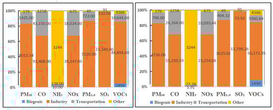
Figure 5.
Proportion of major pollutant emissions by each emission sector in Shanghai during April–May 2021 (left) and April–May 2022 (right) (the emission data in the figure are all expressed in metric tons).
The proportion of major pollutant emissions by each emission sector in Shanghai during April–May 2021 and April–May 2022 is relatively consistent. In terms of PM10, industrial sources have the highest proportion of emissions (2021: 83.32%, 2022: 82.90%), followed by transportation sources (2021: 14.82%, 2022: 13.97%); for PM2.5, industrial sources have the highest proportion of emissions (2021: 86.91%, 2022: 86.97%), followed by transportation sources (2021: 12.26%, 2022: 11.62%); industrial sources contribute significantly to SO2 emissions, accounting for 99.05% in 2021 and 98.82% in 2022; for NOx emissions, industrial sources have the highest proportion (2021: 67.79%, 2022: 68.35%), followed by transportation sources (2021: 31.05%, 2022: 29.67%); NH3 emissions have the highest proportion from other sources (mainly agricultural emissions), accounting for 95.64% in 2021 and 97.50% in 2022; industrial sources have the highest proportion of CO emissions (2021: 67.79%, 2022: 68.48%); for VOCs, biogenic sources accounted for 5.22% in 2021 and 8.33% in 2022, while anthropogenic sources accounted for 94.78% in 2021 and 91.67% in 2022, with industrial VOCs having the highest proportion (2021: 80.54%, 2022: 76.02%).
We assessed the emission reduction levels by comparing the emission ratios of various pollutants in Shanghai between April–May 2021 and April–May 2022. The spatial distribution of these reductions is shown in Figure 6. The reduction in SO2 emissions is evenly distributed across the region, and is related to a decrease in industrial coal consumption during the control period. The spatial variation in NOx emissions primarily exhibits a belt-like pattern, with a significant reduction in emission intensity. This is related to the decrease in industrial and vehicular emissions during the lockdown period. The spatial distribution of CO emissions shows a similar belt-like pattern to that of NOx. Noticeable reductions in NH3 emissions are observed in the central part of Shanghai, and we assumed that agricultural sources were unaffected by the lockdown and the reduction in NH3 emissions is mainly associated with the decrease in vehicle emissions from transportation sources. The changes in VOC emissions are concentrated in the central region of Shanghai, with a significant decrease in emission levels. The reductions in emissions for PM10 and PM2.5 are uniformly distributed across the region.
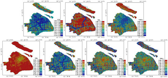
Figure 6.
Spatial distribution of the ratio of total pollutant emissions in Shanghai between April–May 2021 and the same period in 2022 (by comparing the magnitudes of the ratios, the degree of emission reduction can be assessed, with colors ranging from red to blue indicating increasing levels of emission reduction).
Overall, during the lockdown period in 2022, the areas with decreased emissions of SO2, PM10, PM2.5, and NOx show a uniform distribution, while the areas with decreased emissions of VOCs, CO, and NH3 are mainly concentrated in the central region of Shanghai.
3.3. Spatial and Temporal Distribution Characteristics of O3 Concentration during the Lockdown Period
3.3.1. Observational Facts
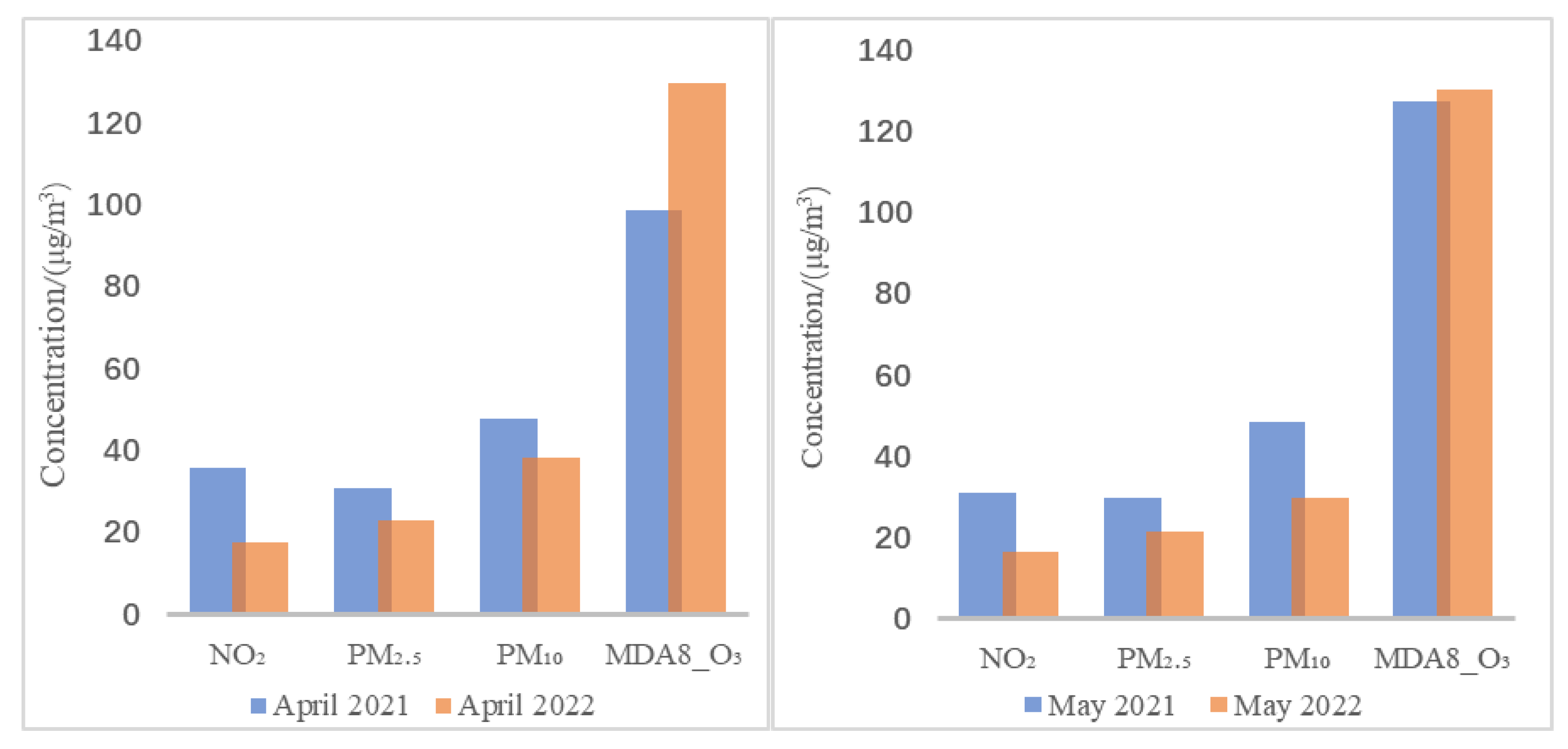
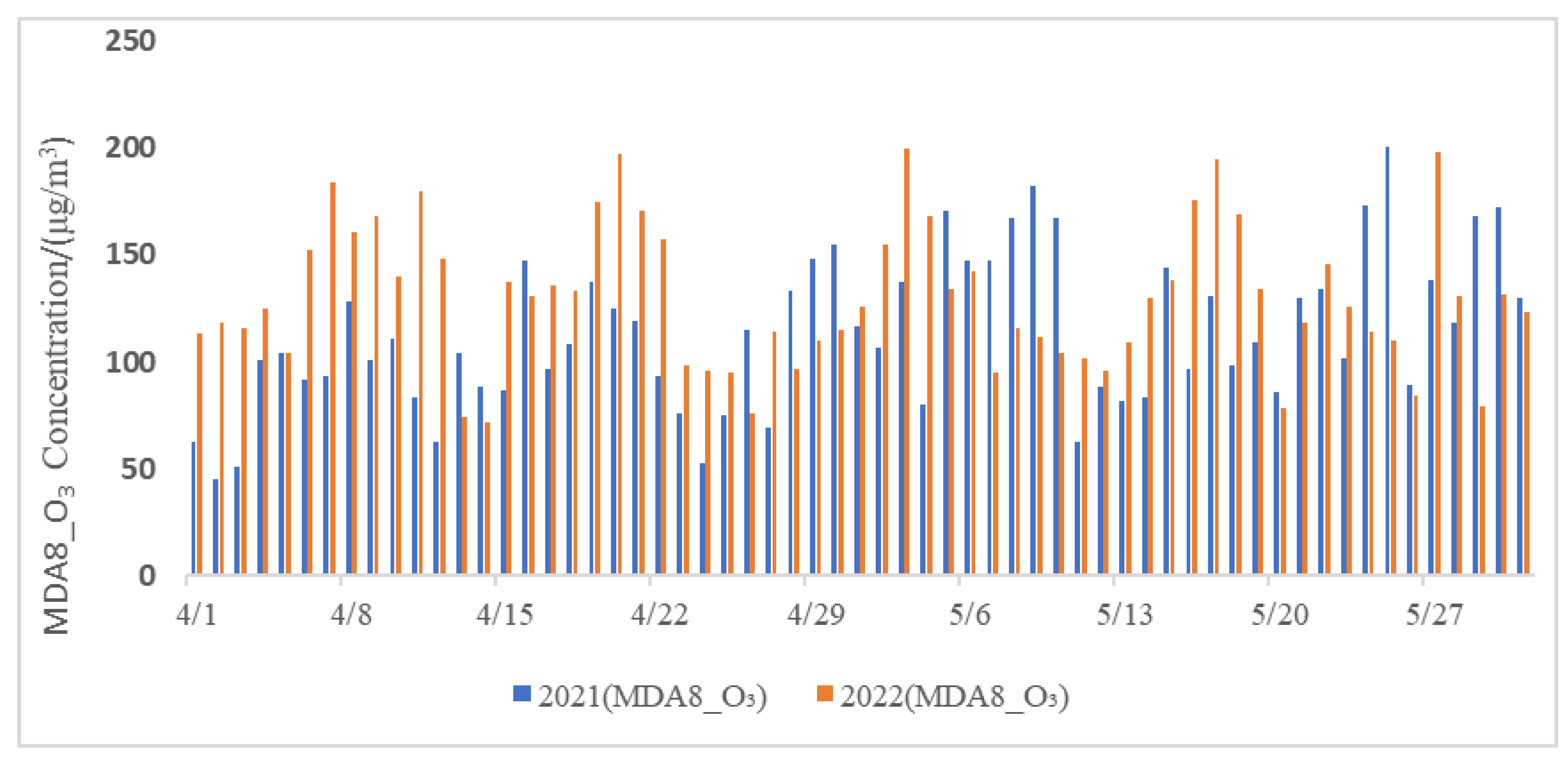
During the lockdown period, due to strict isolation policies, there was a sharp reduction in human activity, which had a significant impact on the atmospheric environment. Comparing the same periods in 2021 and 2022, ground-level monitoring stations observed a significant decrease in the concentrations of several air pollutants, as shown in Figure 7. In April, there was a decrease of 50.42% in NO2, 19.99% in PM10, and 25.68% in PM2.5. In May, there was a decrease of 46.60% in NO2, 38.48% in PM10, and 28.20% in PM2.5. However, the overall air quality in Shanghai did not improve. According to real-time observations, the average Air Quality Index during the lockdown period was 76.90, which was relatively consistent with the average AQI of 70.49 during the same period in 2021. This was primarily due to an increase in the frequency and intensity of O3 pollution, as shown in Figure 8. During the lockdown period, Shanghai experienced consistently high levels of O3 pollution compared to 2021.
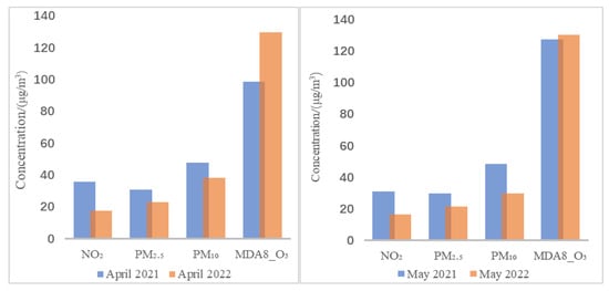
Figure 7.
Monthly average concentrations of NO2, PM2.5, PM10, and MDA8_O3 in April and May of 2021 and 2022.
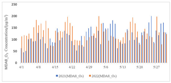
Figure 8.
MDA8_O3 daily average concentrations from 1 April to 31 May in 2021 and 2022.
According to China’s Environmental Air Quality Standards (GB3095-2012) (https://www.mee.gov.cn/, accessed on 9 July 2023), during the lockdown period, from 1 April to 31 May 2022, Shanghai experienced a total of 61 days: there were 49 days during this period when the MDA8 O3 concentration exceeded the primary concentration limit of 100 µg/m3, and 13 days when it exceeded the secondary concentration limit of 160 µg/m3.
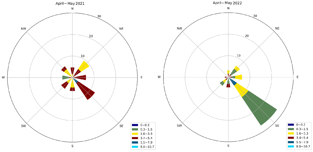
Meteorological conditions generally play a fundamental role in atmospheric pollution. Chang et al. found that high-pressure systems dominated by southwest winds in Shanghai are the most conducive to high concentrations of O3 [28]. In Shanghai, south and southeast winds prevail during the months of April and May. By comparing the wind speed and direction between April–May 2021 and April–May 2022 (Figure 9), we found no significant changes in the wind conditions over Shanghai, and the comparative analysis of temperature trends during this period found that the average high temperatures in April 2021 and 2022 were 21 °C and 22 °C, respectively, while the average low temperatures were 14 °C and 13 °C. In May 2021 and 2022, the average high temperatures were 27 °C and 25 °C, respectively, while the average low temperatures were 19 °C and 17 °C. The meteorological conditions were generally consistent between the two years and did not constitute decisive factors influencing pollution. Consequently, the high concentrations of O3 are primarily attributed to the significant changes in human activities during the lockdown period [29].
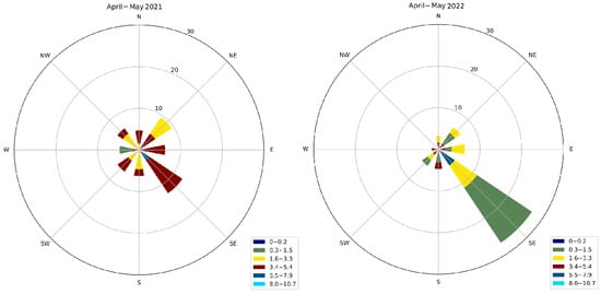
Figure 9.
Wind Speed and Direction Comparison between April–May 2021 and April–May 2022.
3.3.2. Simulation Results
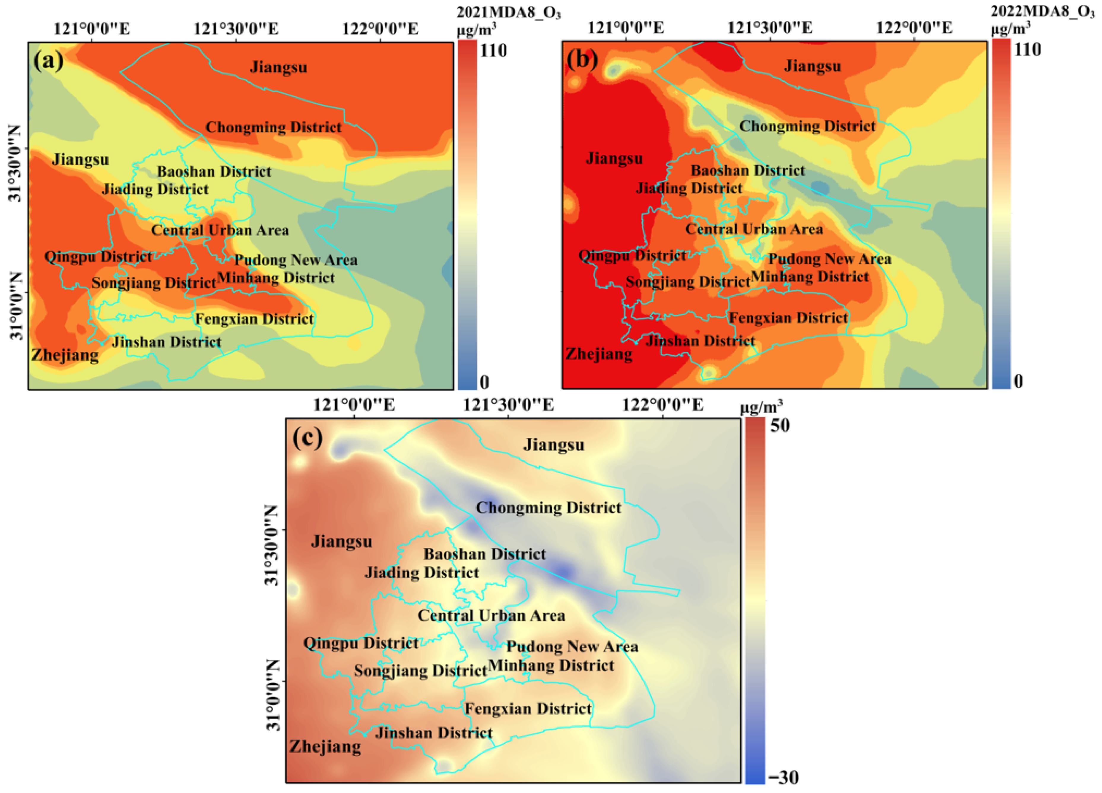
Based on a statistical analysis of simulation results from CAMx, the distribution characteristics of monthly average maximum eight-hour ozone (MDA8 O3) concentrations in the Shanghai area during April and May of 2021 and 2022 are shown in the Figure 10. In April and May 2022, the MDA8 O3 concentrations in Shanghai ranged from 16.92 to 104.03 μg/m3, with a regional average concentration of 79.70 μg/m3. The spatial distribution showed higher ozone concentrations in the western areas of Shanghai and the adjacent Jiangsu and Zhejiang regions, while the central urban area of Shanghai and its eastern regions exhibited lower concentrations. In April and May 2021, the MDA8 O3 concentrations in Shanghai ranged from 7.68 to 88.32 μg/m3, with a regional average concentration of 73.26 μg/m3. The spatial distribution shows that higher ozone concentrations were observed in most areas of Chongming Island and its surrounding regions, as well as in the offshore areas of Jiangsu. The ozone concentrations were the second highest in the central and western parts of Shanghai and the neighboring Jiangsu and Zhejiang regions. Lower ozone concentrations were observed in the southern and eastern areas of Shanghai. Compared to April and May 2021, the MDA8 O3 concentrations in most areas of the Shanghai region (The coastal area in the north of Chongming Island, the area near Jiangsu and Zhejiang provinces, and the eastern area of Shanghai) increased in 2022, with an average increase of 6.44 μg/m3 and a growth rate of 8.79%.
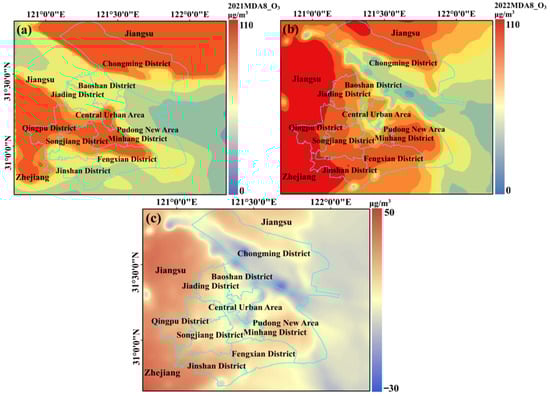
Figure 10.
Monthly average concentration of MDA8 O3 during April and May of 2021 (a) and 2022 (b), and the difference in monthly average concentration of MDA8 O3 between April–May 2022 and the same period in 2021 (c).
3.4. Source Apportionment of O3 during the Lockdown Period
3.4.1. Analysis of the Main Contributors to O3 Precursors
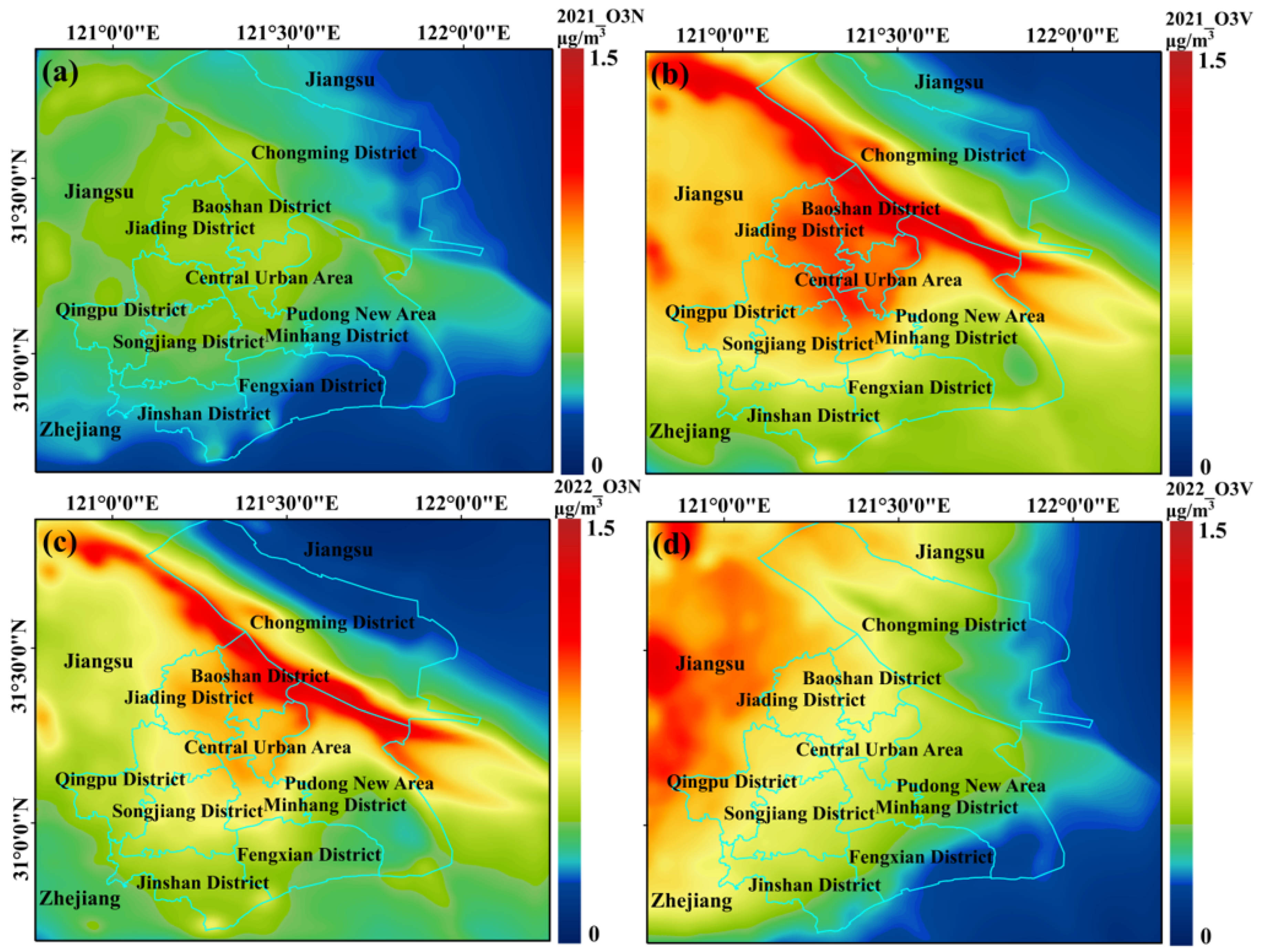
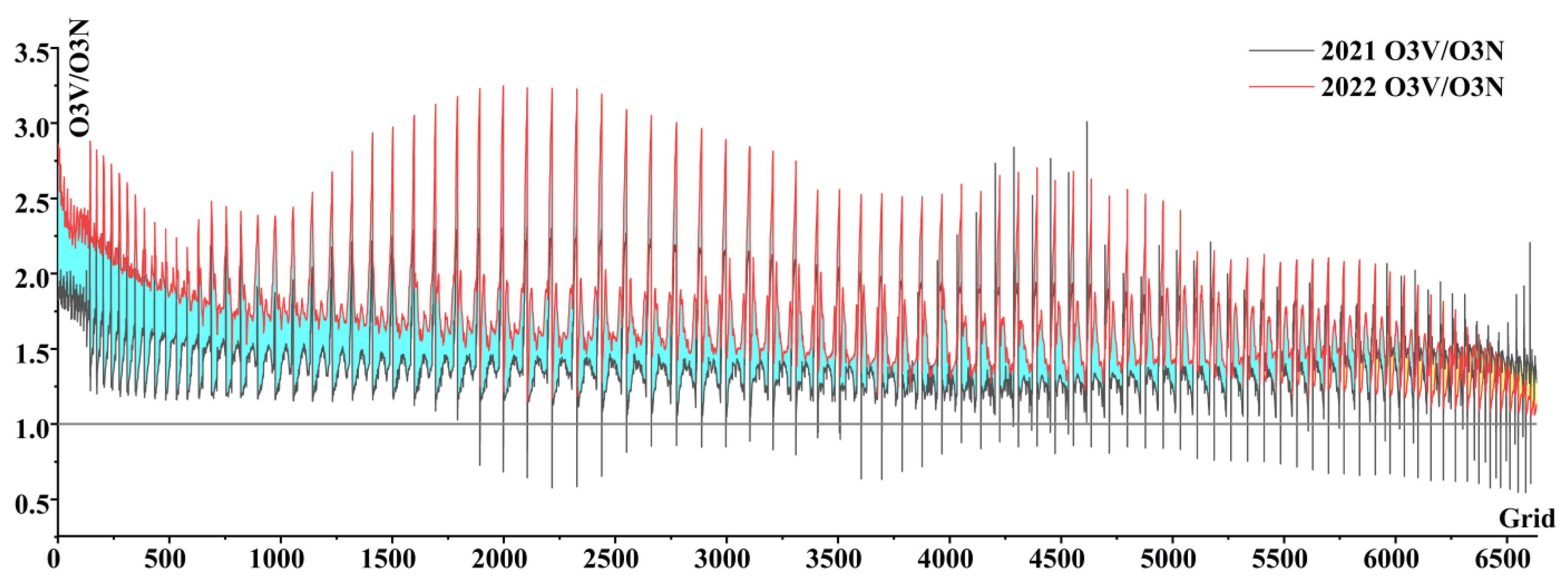
In the CAMx-OSAT model, the ozone formation under NOx control or VOCs control is identified based on the ratio of H2O2 to HNO3 generation rates. O3N and O3V are ozone formation indicators in the OSAT module, representing ozone generated under NOx control conditions and VOCs control conditions, respectively [13]. The ratio between them reflects the ozone formation mechanism in the region. The spatial distribution of the contributions of NOx and VOCs, emitted in the Shanghai region, to O3 generation during the pollution analysis period in 2021 and the corresponding period in 2022, is shown in Figure 11. By extracting the grid cells in the Shanghai area, the sensitivity of ozone formation in Shanghai was investigated based on the ratio of O3V to O3N, as shown in Figure 12. According to the displayed figures, in the entire Shanghai region, during April and May 2021, most areas have O3V/O3N ratios greater than 1, indicating that ozone formation is primarily driven by VOCs, representing the VOCs control zone. However, there are small areas where the O3V/O3N ratio is less than 1, indicating the NOx control zone. In the corresponding period of 2022, the O3V/O3N ratios are greater than 1 throughout the Shanghai region, indicating it as a VOCs control zone. Previous studies have generally indicated that, in urban areas and their immediate vicinity, there is strong NOx emission and higher NOx concentrations, where the reaction between OH radicals and NOx is dominant, resulting in ozone formation primarily under VOCs control [13]. Huang et al. [10] drew O3-VOCs-NOx isopleths (EKMA) based on WRF-Chem simulation results, which indicated that ozone formation in the eastern part of China (30° N–40° N, 110° E–120° E) is VOCs-controlled, and with a reduction in NOx, ozone formation can increase by 40% to 50%. The distribution of ozone precursors in Shanghai in this study aligns with previous research.
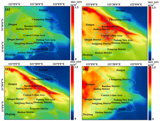
Figure 11.
Contribution of O3N(NOx) and O3V(VOCs) to O3 generation during April and May of 2021 ((a): O3N; (b): O3V) and 2022 ((c): O3N; (d): O3V) (note: O3N represents ozone formed under NOx-limited conditions from NOx emission; O3V represents ozone formed under VOCs-limited conditions from VOCs emission).
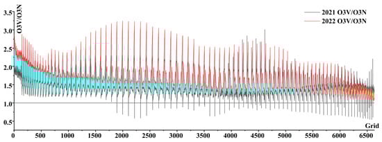
Figure 12.
Ozone formation regimes in Shanghai during April and May of 2021 and 2022 (the horizontal axis represents the number of grids in the Shanghai area within the simulated range, while the vertical axis represents the ratio of O3V to O3N in each selected grid area).
The study by Yin et al. [30] demonstrated that, during the COVID-19 lockdown period in Wuhan, ozone (O3) increased by 43%, with meteorological conditions contributing 6% of the increase. This indicates that the reduction in ozone precursor emissions during the COVID-19 lockdown was the main cause of changes in tropospheric ozone. In urban centers, which are often VOCs-controlled areas, high concentrations of NO have a scavenging effect on ozone. The reduction in NOx, primarily through decreased NO emissions, weakens the scavenging effect, leading to an increase in ozone concentrations [7]. Liu et al. [31] defined the number of ozone molecules produced by removing one NOx molecule as the ozone production efficiency (OPE). During the transport of air masses, as the air masses undergo photochemical aging, the amount of NOx decreases continuously, and OPE shows an increasing trend. The photochemical characteristics within the air masses become more favorable for ozone production [32,33].
Wang [34] used the WRF-Chem model to design 36 emission reduction scenarios based on varying proportions of NOx and VOC reductions. These scenarios simulated the air quality conditions during periods of PM2.5 and O3 combined pollution in the Yangtze River Delta region. Employing a combination of the Comprehensive EKMA Curve (CEKMA) and Dijkstra’s shortest path algorithm, Wang assessed the air quality under different reduction scenarios, considering cost-effectiveness, environmental impacts, health benefits, and spatial effects. This analysis yielded varying effects of synergistic NOx and VOC reductions, and also explored the optimal reduction pathway for NOx and VOC emissions in the Shanghai area: prioritizing NOx reduction first, followed by VOC reduction, and vice versa. Both strategies led to the most effective improvement in air quality, with an improvement efficiency of about 85–100%. Conversely, the simultaneous proportional reduction in NOx and VOCs represented the least optimal pathway, resulting in the least improvement in air quality, with an improvement efficiency of just 77–85%. During the research phase of this study, the reduction ratios for VOCs and NOx emissions, the precursors of ozone, were approximately 39.45% and 41.48%, respectively. This nearly equal proportion of simultaneous reduction was found to be one of the less effective emission reduction strategies for regional air quality improvement.
3.4.2. Analysis of Sector Source Contribution of O3
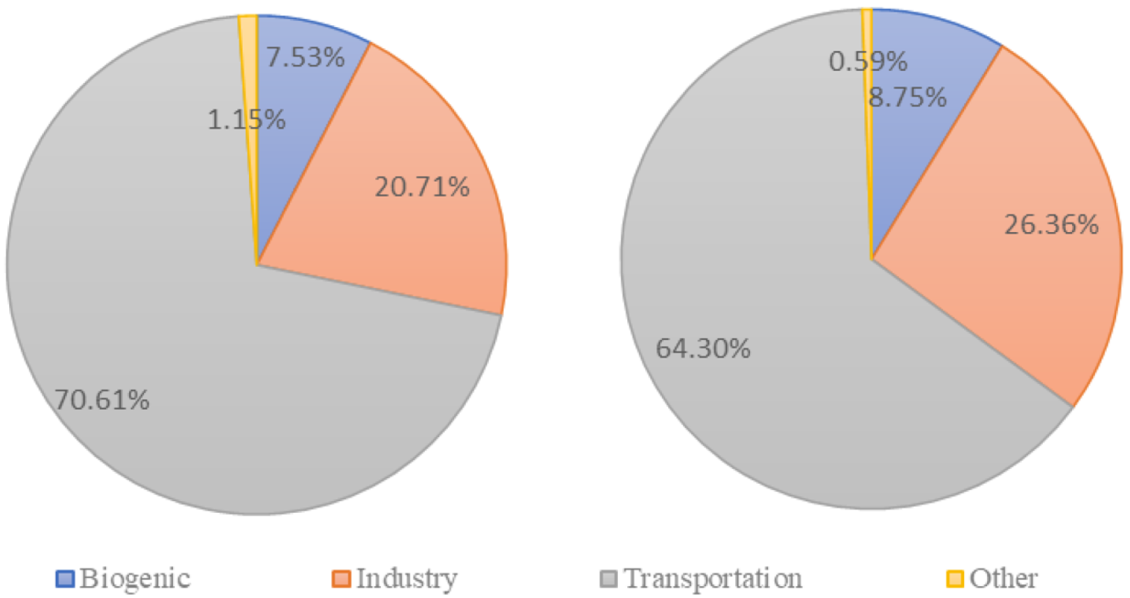
Figure 13 shows the monthly average percentage contributions of four emission sources to MDA8 O3 concentrations in Shanghai during the simulated analysis period. From Figure 13, it can be observed that, during the lockdown period of the COVID-19 pandemic, the transportation sector was the largest contributor to MDA8 O3 concentrations in Shanghai, accounting for MDA8 O3 monthly contribution of 64.30%. The industrial sector ranked second with a monthly average contribution percentage of 26.36%, while natural sources contributed an average of 8.75% to hourly O3 concentrations in Shanghai. Contributions from residential and agricultural sources were relatively small, accounting for only 0.59% of the monthly average MDA8 O3 concentrations. Compared with the same period in 2021, the proportion trend of concentration contribution is similar to that in 2022, but the proportion changes significantly. For example, the proportion of road traffic sources contributing to the ozone concentration has significantly decreased from 70.61% to 64.3%, but it is still the largest contributor. The contribution of industrial emissions to the ozone concentration has significantly risen from 20.71% to 26.36%, making it still the second largest contributor. The pandemic lockdown measures resulted in a reduction in anthropogenic emissions, the decrease in traffic flow during the strict lockdown period led to a decrease in the contribution of transportation sources. Reductions in vehicle emissions can lead to lower concentrations of pollutants such as PM2.5, PM10, CO, and NO2. The decrease in PM2.5 and PM10 concentrations resulted in increased near-surface ultraviolet radiation intensity, promoting the photochemical production of O3. In the industrial sector, the suspension of manufacturing activities during the pandemic and the impact of epidemic prevention measures led to decreased pollutant emissions. The significant reduction in primary emissions such as SO2 and NO2 resulted in a significant increase in O3 concentrations. This, in turn, enhanced the atmospheric oxidation capacity and the formation of secondary aerosols in the Shanghai region. Additionally, stable weather conditions favored the accumulation of O3 mass concentrations, potentially amplifying local O3 pollution [35]. As a result, during the lockdown period, the O3 pollution levels did not decrease significantly and instead saw an increase [36].

Figure 13.
Contribution of sector sources to monthly average concentration of MDA8 O3 in Shanghai during April–May 2021 (left) and April–May 2022 (right).
3.4.3. Analysis of O3 Regional Contribution
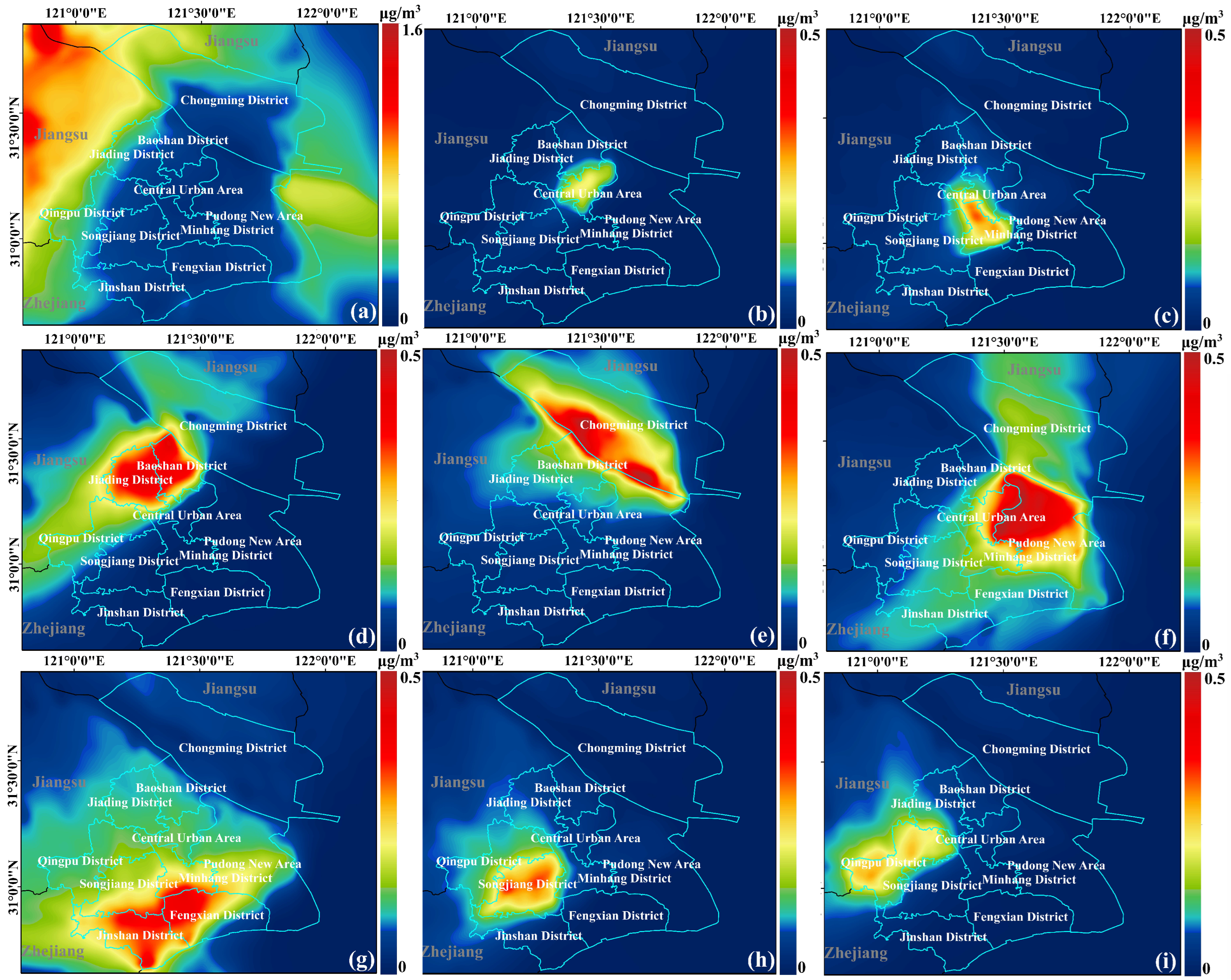
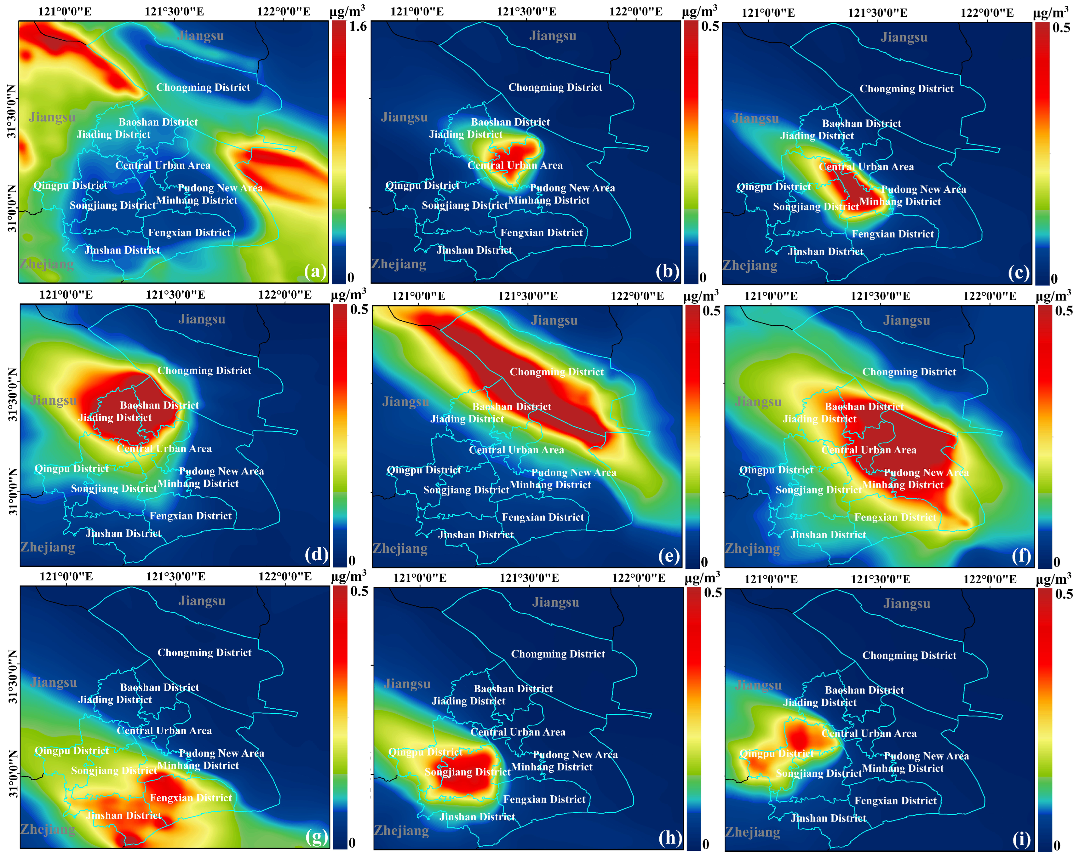
The regional contribution analysis of Shanghai includes nine regions: external areas (regions other than Shanghai), central urban areas (Huangpu District, Jing’an District, Xuhui District, Changning District, Yangpu District, Hongkou District, Putuo District), Minhang District, Baoshan District, Jiading District, Chongming District, Pudong New Area, Jinshan District, Fengxian District, Songjiang District, and Qingpu District. Figure 14 and Figure 15a–i represent the spatial distribution of regional contributions to Shanghai’s O3 concentration during the simulation period for these nine regions. From Figure 14 and Figure 15, it can be observed that different source regions exhibit significant spatial variations in their contributions to ozone concentration. In April–May 2021, the high-contribution regions of local sources to Shanghai’s O3 concentration were primarily concentrated in the southern part of Chongming District, the northern area of Pudong New Area, Jiading District, Baoshan District, western Fengxian District, and the northern and southern parts of Jinshan District. In April–May 2022, the high-contribution regions of local sources to Shanghai’s O3 concentration were mainly concentrated in most areas of Chongming Island, Jiading District, Baoshan District, Minhang District, and the northern and central parts of Pudong New Area. Within these high-contribution regions, the high-value area in Chongming District exhibited a belt-like distribution, while the other high-value areas showed a patchy distribution.

Figure 14.
Contribution of regional sources to O3 pollution in Shanghai in April–May 2021 (a–i) represent External Transport (areas outside Shanghai), Central Urban Area (Huangpu District, Jing’an District, Xuhui District, Changning District, Yangpu District, Hongkou District, Putuo District), Minhang District, Baoshan District and Jiading District, Chongming District, Pudong New Area, Jinshan District and Fengxian District, Songjiang District, and Qingpu District).
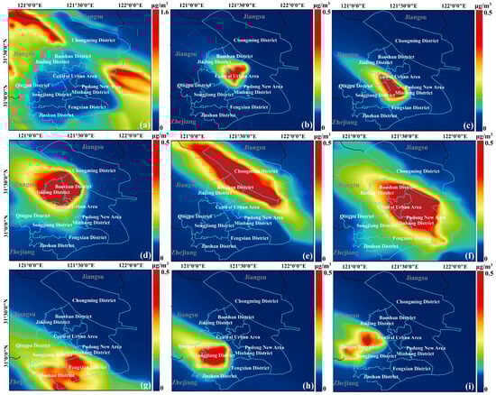
Figure 15.
Contribution of regional sources to O3 pollution in Shanghai in April–May 2022.(a–i) represent External Transport (areas outside Shanghai), Central Urban Area (Huangpu District, Jing’an District, Xuhui District, Changning District, Yangpu District, Hongkou District, Putuo District), Minhang District, Baoshan District and Jiading District, Chongming District, Pudong New Area, Jinshan District and Fengxian District, Songjiang District, and Qingpu District).
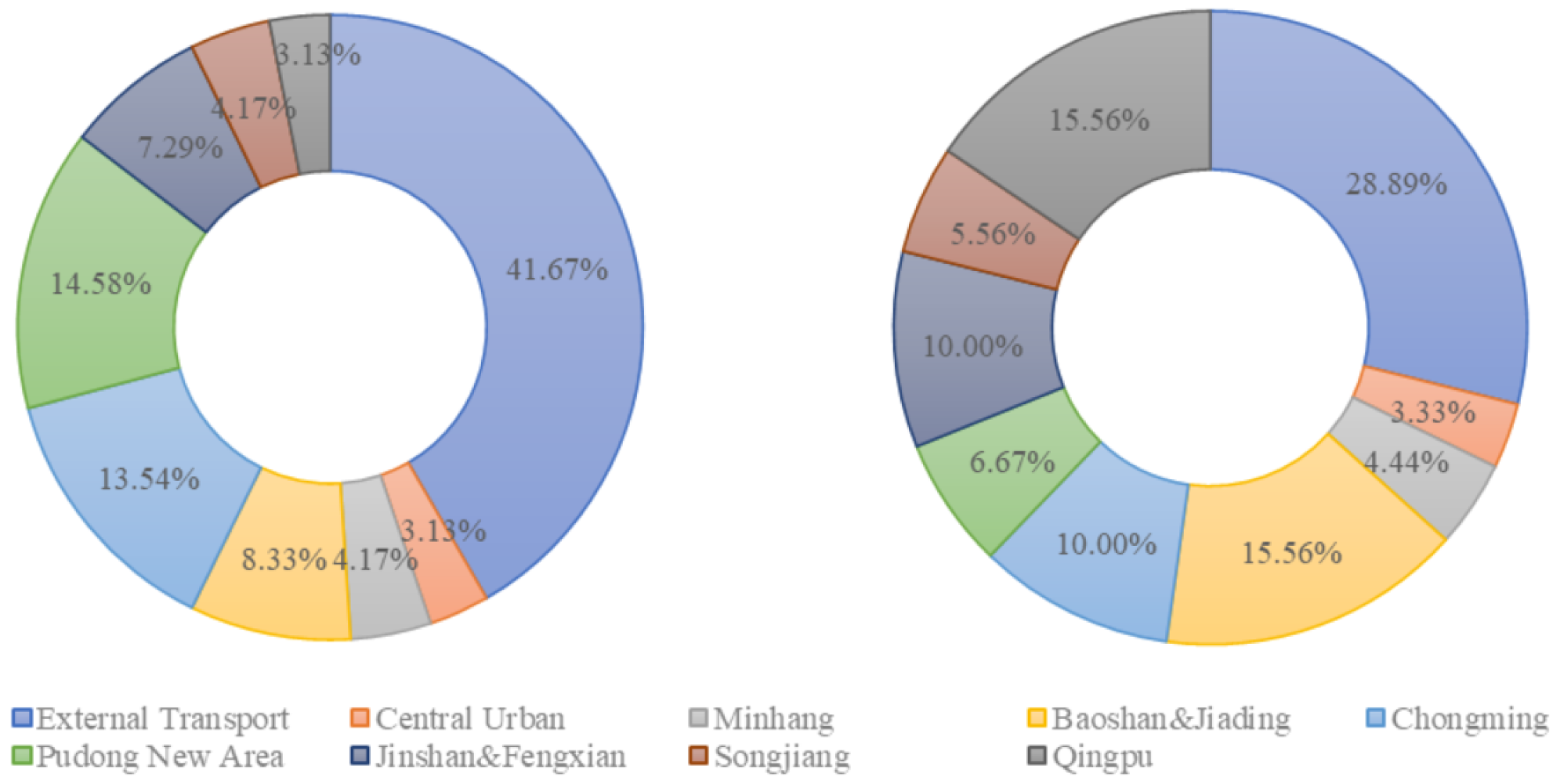
As shown in Figure 16, during April–May 2021, the contribution of local sources to Shanghai’s O3 concentration accounted for 58.33%, while the contribution from external transmission was 41.67%, with a ratio of approximately 6:4. The main regions contributing to O3 formation were Pudong New Area, Chongming District, Jinshan District, and Fengxian District, accounting for around 35.41%. In the same period of 2022, the contribution of local sources increased to 71.11%, and external transmission contributed 28.89%, with a ratio of about 7:3. Among local sources in Shanghai, Qingpu District, Chongming District, Baoshan District, and Jiading District were the primary contributors to O3 formation, accounting for approximately 41.12%. Local ozone generation remains the primary source of Shanghai’s ozone concentration, emphasizing the significance of controlling local source emissions to manage ozone levels in the region.

Figure 16.
Contribution of regional sources to monthly average concentration of MDA8 O3 in Shanghai during April–May 2021 (left) and April–May 2022 (right).
Generally speaking, during April–May of 2021 and 2022, regional transmission and long-range transport were significant contributors to Shanghai’s ozone concentration. For instance, the southern area of Fengxian, adjacent to Hangzhou Bay, is near a coastal industrial belt consisting of the Cixi, Zhenhai, and Beilun districts, which are dominated by industrial emissions like VOCs. These emissions might be transported to areas on the northern side of Hangzhou Bay, such as Jinshan, and jointly influenced by local sources, causing higher O3 values when the wind direction is southerly. Ozone from outside the Shanghai area, transported through regional transmission, could affect the sensitivity of ozone to local precursor emissions, potentially impacting the effectiveness of controlling ozone concentrations through local precursor reduction.
When PM2.5 emission contributions decrease, the concentrations of hydrogen peroxide radicals (HO2·) and nitrogen oxide radicals (NOx·≡NO+NO2) in the air increase. This leads to elevated levels of hydroxyl radicals (HOx·≡OH·+HO2·+RO2·) and nitrogen oxide radicals, promoting the catalytic oxidation of volatile organic compounds (VOCs) by NOx· and HOx·, resulting in the generation of O3 and its accumulation [37]. The Shanghai Environmental Monitoring Center [38] divides the administrative divisions of Shanghai into three major regions based on the inner and outer ring roads: within the inner ring road, between the inner and outer ring roads, and outside the outer ring road. The area outside the outer ring road is the main region of pollutant emissions in Shanghai, with a contribution rate of 58.9% for PM2.5 emissions. During the lockdown period, there was a significant reduction in PM2.5 emissions outside the outer ring road, resulting in significantly higher O3 emission contributions in these four regions (Qingpu District, Chongming District, Baoshan District, and Jiading District) compared to the rest of the areas.
4. Conclusions
The lockdown measures that occurred in Shanghai from April to May 2022 provided an “ideal air quality experiment” for pollution research. This paper conducted a simulation study to analyze the characteristics of ozone pollution, sources of high ozone concentrations, and ozone formation mechanisms during the lockdown period in Shanghai. The main conclusions are as follows:
- (1)
- During the lockdown period, the air quality in Shanghai showed significant differences compared to non-lockdown periods, the concentrations of most pollutants generally decreased, while the ozone concentration increased. By comparing the PM2.5 and O3 monitoring data for Shanghai from 1 April to 31 May 2022 (a total of 61 days) with the same period in 2021, it was found that the average PM2.5 concentration in Shanghai decreased by 26.8% during this period. However, the MDA8 O3 concentration increased by 14.5%. A total of 49 days had MDA8 O3 concentrations exceeding the first-level concentration limit (100 µg/m³), and 13 days exceeded the prescribed second-level concentration limit (160 µg/m³);
- (2)
- The controlled simulation results of O3 precursors in Shanghai indicate the following: During the simulated period of 2021, the majority of Shanghai’s O3 was primarily influenced by VOCs (volatile organic compounds) in most areas, while in certain suburban counties and rural regions of the city, ozone formation was mainly driven by NOx (nitrogen oxides) control. However, during the simulated period of 2022, the generation of ozone in Shanghai was predominantly driven by VOCs, and the entire area was under VOCs control. Generally speaking, controlling VOCs is an effective approach to reduce O3 concentrations in Shanghai;
- (3)
- A sector source analysis revealed that the transportation sector contributes the most to O3 formation in Shanghai, accounting for 70.61% in 2021 and 64.30% in 2022. Following transportation, the industrial sector also plays a significant role, contributing 20.71% and 26.36% in the respective years. Therefore, controlling emissions from the transportation and industrial sectors should be a priority;
- (4)
- Shanghai’s regional source apportionment results indicate the following: During the months of April and May in 2021, local sources accounted for 58.33% of the contribution to Shanghai’s O3 concentration, while contributions from sources outside the region accounted for 41.67%. The ratio between local sources and transboundary transport was approximately 6:4. In the same period in 2022, local sources contributed to 71.11% of Shanghai’s O3 concentration, while contributions from sources outside the region accounted for 28.89%. The local sources to transboundary transport ratio increased to about 7:3, indicating an elevated contribution from local sources. Locally generated ozone is the primary source of Shanghai’s ozone concentration, and controlling emissions from local sources is the key to managing ozone levels in the Shanghai region;
- (5)
- Different source regions exhibit significant spatial variations in their contributions to the ozone concentration. In 2021, high-contribution regions of local sources to Shanghai’s O3 concentration were mainly concentrated in the southern part of Chongming District, the northern area of Pudong New Area, Jiading District, Baoshan District, the western part of Fengxian District, and the northern and southern parts of Jinshan District. In 2022, high-contribution regions of local sources to Shanghai’s O3 concentration were primarily concentrated in most areas of Chongming Island, Jiading District, Baoshan District, Minhang District, and the northern and central parts of Pudong New Area. Among these high-contribution regions, Chongming District’s high-contribution area exhibited a belt-like distribution, while other high-contribution areas showed a patchy distribution.
Despite the positive impact of reduced economic activities on the air quality during the COVID-19 pandemic, the increasing trend of O3 concentration demands attention. This is primarily due to the weakened titration effect of NO on O3 resulting from the reduction in NOx emissions. This indicates that controlling NOx emissions alone, especially from vehicle emissions, is insufficient to effectively regulate near-surface O3 concentrations. Thus, implementing measures that focus on NOx emissions and coordinated VOCs control, based on the sensitivity of O3 chemistry, are essential for O3 control. Further research and analysis of O3 generation mechanisms and the influence of other factors are crucial for developing targeted pollution control strategies and environmental management measures.
Supplementary Materials
The following supporting information can be downloaded at: https://www.mdpi.com/article/10.3390/atmos14101563/s1. Table S1: The parameterization scheme of WRF and CAMx; Table S2: Shanghai’s monthly statistical data used in this study and monthly growth rates (%) in 2022 compared to the same month of 2021 in Shanghai.
Author Contributions
Writing—original draft, writing-review and editing, visualization, S.S.; Software, L.H.; data curation, investigation, W.C.; resources, data curation, S.C.; supervision, methodology, project administration, W.M. All authors have read and agreed to the published version of the manuscript.
Funding
This research received no external funding.
Data Availability Statement
Data is contained within the article or Supplementary Material.
Conflicts of Interest
The authors declare no conflict of interest.
References
- Zhang, J.X.; Han, J.J.; Yin, L.; Zheng, J.W.; Gan, Y.N.; Wang, S.G. Study on the Effect of Atmospheric Environment Improvement during Epidemic Control in Major Cities in China. Environ. Monit. China 2022, 38, 123–133. [Google Scholar]
- Hou, X.W.; Zhu, B. Progress of Research on Global Tropospheric Ozone Variation Characteristics during COVID-19 Pandemic. Clim. Environ. Res. 2023, 28, 103–116. [Google Scholar]
- Mills, G.; Hayes, F.; Simpson, D.; Emberson, L.; Norris, D.; Harmens, H.; Bueker, P. Evidence of widespread effects of ozone on crops and (semi-)natural vegetation in Europe (1990–2006) in relation to AOT40-and flux-based risk maps. Glob. Chang. Biol. 2011, 17, 592–613. [Google Scholar] [CrossRef]
- Nuvolone, D.; Petri, D.; Voller, F. The effects of ozone on human health. Env. Sci. Pollut. Res. Int. 2018, 25, 8074–8088. [Google Scholar] [CrossRef]
- Pusede, S.E.; Cohen, R.C. On the observed response of ozone to NOx and VOC reactivity reductions in San Joaquin Valley California 1995–present. Atmos. Chem. Phys. 2012, 12, 8323–8339. [Google Scholar] [CrossRef]
- Zeng, P.; Lyu, X.P.; Guo, H.; Cheng, H.R.; Jiang, F.; Pan, W.Z.; Wang, Z.W.; Liang, S.W.; Hu, Y.Q. Causes of ozone pollution in summer in Wuhan, Central China. Environ. Pollut. 2018, 241, 852–861. [Google Scholar] [CrossRef] [PubMed]
- Sicard, P.; Paoletti, E.; Agathokleous, E.; Araminienė, V.; Proietti, C.; Coulibaly, F.; De Marco, A. Ozone weekend effect in cities: Deep insights for urban air pollution control. Environ. Res. 2020, 191, 110193. [Google Scholar] [CrossRef] [PubMed]
- Wolff, G.T.; Kahlbaum, D.F.; Heuss, J.M. The vanishing ozone weekday/weekend effect. J. Air Waste Manag. Assoc. 2013, 63, 292–299. [Google Scholar] [CrossRef]
- Tanvir, A.; Javed, Z.; Jian, Z.; Zhang, S.; Bilal, M.; Xue, R.; Wang, S.; Bin, Z. Ground-Based MAX-DOAS Observations of Tropospheric NO2 and HCHO during COVID-19 Lockdown and Spring Festival over Shanghai, China. Remote Sens. 2021, 13, 488. [Google Scholar] [CrossRef]
- Huang, X.; Ding, A.; Gao, J.; Zheng, B.; Zhou, D.; Qi, X.; Tang, R.; Wang, J.; Ren, C.; Nie, W.; et al. Enhanced secondary pollution offset reduction of primary emissions during COVID-19 lockdown in China. Natl. Sci. Rev. 2021, 8, nwaa137. [Google Scholar] [CrossRef]
- Wang, H.; Tan, Y.; Zhang, L.; Shen, L.; Zhao, T.; Dai, Q.; Guan, T.; Ke, Y.; Li, X. Characteristics of air quality in different climatic zones of China during the COVID-19 lockdown. Atmos. Pollut. Res. 2021, 12, 101247. [Google Scholar] [CrossRef] [PubMed]
- Wang, D.Y.; Wang, T.J.; Han, J.C.; Xie, X.D.; Chen, C.; Cao, Y.Q.; Shu, L. Source apportionment of PM2.5 under heavy air pollution conditions in “2 + 26” cities. China Environ. Sci. 2020, 40, 92–99. [Google Scholar]
- Wang, X.S.; Li, J.L.; Zhang, Y.H.; Xie, S.D.; Tang, X.Y. Ozone source attribution during a severe photochemical smog episode in Beijing, China. Sci. China Ser. B Chem. 2009, 39, 548–559. [Google Scholar] [CrossRef]
- Pan, B.; Cheng, L.; Wang, J.; Li, W.; Gu, P.; Xu, R.; Gong, Z. Characteristics and Source Attribution of Ozone Pollution in Beijing-Tianjin-Hebei Region. Environ. Monit. China 2016, 32, 17–23. [Google Scholar]
- Wang, Y.J.; Li, L.; Feng, J.L.; Huang, C.; Huang, H.; Chen, C.; Wang, H. Source apportionment of ozone in the summer of 2010 in Shanghai using OSAT method. Acta Sci. Circumstantiae 2014, 34, 567–573. [Google Scholar]
- Wang, Q.L.; Dong, M.L.; Li, S.J.; Wu, C.Z.; Wang, G.; Chen, B.X.; Li, W.; Gao, X.; Ye, R.M. Characteristics of Ozone Pollution Distribution and Source Apportionment in Zhoushan. Huanjing Kexue 2019, 40, 1143–1151. [Google Scholar]
- Gao, J.H.; Bin, Z.; Xiao, H.; Kang, H.Q.; Hou, X.W.; Shao, P. A case study of surface ozone source apportionment during a high concentration episode, under frequent shifting wind conditions over the Yangtze River Delta, China. Sci. Total Environ. 2016, 544, 853–863. [Google Scholar] [CrossRef]
- Wang, Q.; Wang, X.; Huang, R.; Wu, J.; Xiao, Y.; Hu, M.; Fu, Q.; Duan, Y.; Chen, J. Regional Transport of PM2.5 and O-3 Based on Complex Network Method and Chemical Transport Model in the Yangtze River Delta, China. J. Geophys. Res. Atmos. 2022, 127, e2021JD034807. [Google Scholar] [CrossRef]
- Liang, Y.X.; Yin, K.H.; Hu, Y.T.; Liu, B.Z.; Liao, R.; Yan, M. Sensitivity analysis of ozone precursor emission in Shenzhen, China. China Environ. Sci. 2014, 34, 1390–1396. [Google Scholar]
- Shen, J.; Chen, H.; Zhong, L.J. Ozone source apportionment in the Pearl River Delta in autumn. Environ. Pollut. Control 2015, 37, 25–30. [Google Scholar]
- Li, Y.; Lau, A.K.H.; Fung, J.C.H.; Zheng, J.Y.; Zhong, L.J.; Louie, P.K.K. Ozone source apportionment (OSAT) to differentiate local regional and super-regional source contributions in the Pearl River Delta region, China. J. Geophys. Res. Atmos. 2012, 117, D15305. [Google Scholar] [CrossRef]
- Chen, H.; Wang, X.S.; Shen, J.; Lu, K.D.; Zhang, Y.H. Ozone Source Apportionment of Typical Photochemical Pollution Episodes in the Pearl River Delta in Autumn. Acta Sci. Nat. Univ. Pekin. 2015, 51, 620–630. [Google Scholar]
- Xue, W.; Fu, F.; Wang, J.; Tang, G.; Lei, Y.; Yang, J.; Wang, Y. Numerical study on the characteristics of regional transport of PM2.5 in China. China Environ. Sci. 2014, 34, 1361–1368. [Google Scholar]
- Dunker, A.M.; Koo, B.; Yarwood, G. Contributions of foreign, domestic and natural emissions to US ozone estimated using the path-integral method in CAMx nested within GEOS-Chem. Atmos. Chem. Phys. 2017, 17, 12553–12571. [Google Scholar] [CrossRef]
- Chen, K.; Wang, P.; Zhao, H.; Wang, P.; Gao, A.; Myllyvirta, L.; Zhang, H. Summertime O3 and related health risks in the north China plain: A modeling study using two anthropogenic emission inventories. Atmos. Environ. 2021, 246, 118087. [Google Scholar] [CrossRef]
- Uranishi, K.; Ikemori, F.; Nakatsubo, R.; Shimadera, H.; Kondo, A.; Kikutani, Y.; Asano, K.; Sugata, S. Identification of biased sectors in emission data using a combination of chemical transport model and receptor model. Atmos. Environ. 2017, 166, 166–181. [Google Scholar] [CrossRef]
- Liu, X.-H.; Zhang, Y.; Cheng, S.-H.; Xing, J.; Zhang, Q.; Streets, D.G.; Jang, C.; Wang, W.-X.; Hao, J.-M. Understanding of regional air pollution over China using CMAQ, part I performance evaluation and seasonal variation. Atmos. Environ. 2010, 44, 2415–2426. [Google Scholar] [CrossRef]
- Chang, L.Y.; He, F.F.; Tie, X.X.; Xu, J.M.; Gao, W. Meteorology driving the highest ozone level occurred during mid-spring to early summer in Shanghai, China. Sci. Total Environ. 2021, 785, 147253. [Google Scholar] [CrossRef]
- Xue, R.; Wang, S.; Zhang, S.; Zhan, J.; Zhu, J.; Gu, C.; Zhou, B. Ozone Pollution of Megacity Shanghai during City-Wide Lockdown Assessed Using TROPOMI Observations of NO2 and HCHO. Remote Sens. 2022, 14, 6344. [Google Scholar] [CrossRef]
- Yin, H.; Liu, C.; Hu, Q.; Liu, T.; Wang, S.; Gao, M.; Xu, S.; Zhang, C.; Su, W. Opposite impact of emission reduction during the COVID-19 lockdown period on the surface concentrations of PM2.5 and O3 in Wuhan, China. Environ. Pollut. 2021, 289, 117899. [Google Scholar] [CrossRef]
- Liu, S.C.; Trainer, M.; Fehsenfeld, F.C.; Parrish, D.D.; Williams, E.J.; Fahey, D.W.; Hübler, G.; Murphy, P.C. Ozone production in the rural troposphere and the implications for regional and global ozone distributions. J. Geophys. Res. Atmos. 1987, 92, 4191–4207. [Google Scholar] [CrossRef]
- Kleinman, L.I.; Daum, P.H.; Lee, Y.N.; Nunnermacker, L.J.; Springston, S.R.; Weinstein-Lloyd, J.; Rudolph, J. Ozone production efficiency in an urban area. J. Geophys. Res. Atmos. 2002, 107, ACH 23-1–ACH 23-12. [Google Scholar] [CrossRef]
- Zaveri, R.A. Ozone production efficiency and NOxdepletion in an urban plume: Interpretation of field observations and implications for evaluating O3-NOx-VOC sensitivity. J. Geophys. Res. 2003, 108, D14. [Google Scholar]
- Wang, J.Y. Research on the Collaborative Control of O3 and PM2.5 Pollution in the Yangtze River Delta Region. East China Norm. Univ. 2022, 12, 74. [Google Scholar]
- Zhang, L.; Wang, T.; Zhang, Q.; Zheng, J.Y.; Xu, Z.; Lv, M.Y. Potential sources of nitrous acid (HONO) and their impacts on ozone: A WRF-Chem study in a polluted subtropical region. J. Geophys. Res. Atmos. 2016, 121, 3645–3662. [Google Scholar] [CrossRef]
- Kuang, Y.Q.; Zou, Z.; Zhang, X.Y.; Chang, Y.H. Spatial-temporal responses of atmospheric pollutants to the COVID-19 lockdown across the Yangtze River Delta region. Acta Sci. Circumstantiae 2021, 41, 1165–1172. [Google Scholar]
- Li, K.; Jacob, D.J.; Liao, H.; Qiu, Y.; Shen, L.; Zhai, S.; Bates, K.H.; Sulprizio, M.P.; Song, S.; Lu, X.; et al. Ozone pollution in the North China Plain spreading into the late-winter haze season. Proc. Natl. Acad. Sci. USA 2021, 118, e2015797118. [Google Scholar] [CrossRef]
- Fu, Q.Y.; Lu, T.; Wu, Y.M.; Gao, S.; Wei, H.P. Research on major air pollutant emission sources and emission sharing rate in Shanghai. In Proceedings of the 4th China (International) Forum on Environment and Development, Beijing, China, 18–19 October 2008; pp. 300–308. [Google Scholar]

Disclaimer/Publisher’s Note: The statements, opinions and data contained in all publications are solely those of the individual author(s) and contributor(s) and not of MDPI and/or the editor(s). MDPI and/or the editor(s) disclaim responsibility for any injury to people or property resulting from any ideas, methods, instructions or products referred to in the content. |
© 2023 by the authors. Licensee MDPI, Basel, Switzerland. This article is an open access article distributed under the terms and conditions of the Creative Commons Attribution (CC BY) license (https://creativecommons.org/licenses/by/4.0/).