Abstract
Observations of precipitable water vapor (PWV) in the atmosphere play a crucial role in weather forecasting and global climate change research. Spaceborne Interferometric Synthetic Aperture Radar (InSAR), as a widely used modern geodetic technique, offers several advantages to the mapping of PWV, including all-weather capability, high accuracy, high resolution, and spatial continuity. In the process of PWV retrieval by using InSAR, accurately extracting the tropospheric wet delay phase and obtaining a high-precision tropospheric water vapor conversion factor are critical steps. Furthermore, the observations of InSAR are spatio-temporal differential results and the conversion of differential PWV (InSAR ΔPWV) into non-difference PWV (InSAR PWV) is a difficulty. In this study, the city of Jinan, Shandong Province, China is selected as the experimental area, and Sentinel-1A data in 2020 is used for mapping InSAR ΔPWV. The method of small baseline subset of interferometry (SBAS) is adopted in the data processing for improving the coherence of the interferograms. We extract the atmosphere phase delay from the interferograms by using SRTM-DEM and POD data. In order to evaluate the calculation of hydrostatic delay by using the ERA5 data, we compared it with the hydrostatic delay calculated by the Saastamoinen model. To obtain a more accurate water vapor conversion factor, the value of the weighted average temperature Tm was calculated by the path integral of the ERA5. In addition, GNSS PWV is used to calibrate InSAR PWV. This study demonstrates a robust consistency between InSAR PWV and GNSS PWV, with a correlation coefficient of 0.96 and a root-mean-square error (RMSE) of 1.62 mm. In conclusion, our method ensures the reliability of mapping PWV by using Sentinel-1A interferograms and GNSS observations.
1. Introduction
Precipitable water vapor (PWV) refers to the amount of precipitation that could potentially descend to the ground. It can be generated by the condensation of water vapor per unit area of the atmospheric column from the ground to the top of the atmosphere. It has a great significance in monitoring and predicting weather and studying global climate change [1,2,3]. Interferometric Synthetic Aperture Radar (InSAR), as a rapidly developing geodetic technology, has the characteristics of all weather, large scale, and high resolution [4,5,6,7]. Spaceborne InSAR obtains interferometric phase maps by subtracting the echo phase of the corresponding pixels of two or more SAR images covering the same area [8,9,10,11]. An interferogram between two SAR images is impacted by contributions from the atmosphere, the surface deformation, topography, and other sources of noise [12,13,14,15]. The atmospheric delay in the interferograms can be utilized as the research object to retrieve spatially continuous PWV [16,17,18,19].
The total tropospheric delay consists of the wet delay and the hydrostatic delay [20,21]. Therefore, accurately obtaining the hydrostatic delay is equivalent to accurately obtaining the wet delay. The variation in hydrostatic delay is closely related to changes in atmospheric pressure. Within a spatial range of 100 km × 100 km, the change in atmospheric pressure is less than 1 hPa. The spatio-temporal variations of atmospheric pressure are relatively stable. Therefore, the hydrostatic delay remains stable over time. As a result, the hydrostatic delay on interferograms is often ignored in many studies. However, studies by previous researchers have shown that, in some terrains, although the temporal variation in atmospheric pressure is small, it can be within 10% of the total atmospheric pressure. This results in centimeter-level differences in hydrostatic delay when differencing interferograms at different times [22]. Furthermore, the swath of InSAR data in this study was 250 km. In these larger-scale interferograms, spatial variations in atmospheric pressure can cause hydrostatic delay differences that exhibit characteristics related to the topography. The magnitude of this impact depends on the elevation and the prevailing meteorological conditions at the image acquisition time. Consequently, the hydrostatic delay in interferograms cannot be disregarded.
The water vapor conversion factor is an essential parameter for converting zenith wet delay into PWV. It depends on the mean temperature profiles, varying with season, weather, and specific location, which leads to the value varying by as much as 10% [23]. The water vapor conversion factor typically falls between 6.0 and 6.5, but can reach 7.0 under extreme weather conditions [24]. Many studies assume a constant value for the water vapor conversion factor, but this assumption is not valid in scenarios where a high-accuracy PWV is required [25]. Hence, accurately determining the water vapor conversion factor for each pixel in an interferogram becomes one of the key question to achieve the precise atmospheric water vapor. The water vapor conversion factor is a function of the weighted average temperature. Therefore, accurately calculating the weighted average temperature is a crucial step in obtaining water vapor conversion factors. Generally, there are two common methods for calculating the weighted average temperature: the numerical integration method using radiosonde data and the empirical regression model method [26,27]. The former is currently the most accurate method for calculating the weighted average temperature. Meteorological radiosonde stations are sparsely distributed, typically around 300 km apart, and they perform observations only twice a day (morning and evening), resulting in a lower temporal and spatial resolution [28]. This is insufficient to meet the requirements for InSAR PWV. In practical applications, statistical regression methods are generally employed to establish a functional relationship between the water vapor conversion factor and latitude, day of year. The commonly used model is the Bevis weighted average temperature empirical model [29]. Due to regional differences, applying a water vapor inversion based on data from global regions can introduce regional model system errors, leading to suboptimal atmospheric water vapor estimations. Therefore, many researchers use local meteorological data from radiosonde stations and statistical analysis methods to develop more region-specific weighted average temperature calculation models [30]. However, meteorological data from radiosonde stations are not spatially continuous, making it impossible to obtain spatially continuous weighted average temperatures. ERA5, the latest ECMWF reanalysis, provides a comprehensive record of the global atmosphere, land surface, and ocean waves [31]. This system is based on the ECMWF Integrated Forecasting System (IFS) Cy41r2, and its assimilation system uses short-range forecasts from 06:00 and 18:00 UTC for assimilating observations [32]. Compared to radiosonde data, ERA5 data (relative humidity, temperature, and geopotential) are spatially continuous. It can be used to obtain spatially continuous weighted average temperatures.
In addition, the InSAR-derived PWV is ∆PWV between the imaging time of the master image and the slave image. To address this issue, some studies have proposed a method that combines ENVISAT-ASAR and ENVISAT-MERIS for PWV retrieval. ENVISAT-ASAR and ENVISAT-MERIS are two sensors installed on the same ENVISAT satellite. The water vapor observation data from ENVISAT-MERIS can be used as synchronous observational data for ENVISAT-ASAR in the calibration process [33]. However, many satellites lack synchronous water vapor observational data. In response to the issue of a lack of synchronized observations of water vapor data, some scholars have conducted explorations. Some researchers proposed to merge the global atmospheric reanalysis simulations and GPS data to obtain the non-differential PWV at different SAR acquisitions in time and space [34,35]. The BeiDou Navigation Satellite System (BDS) officially provides a global service since July 2020. BDS includes 3 geostationary orbit (GEO) satellites, 3 inclined geosynchronous orbit (IGEO) satellites, and 24 medium Earth orbit (MEO) satellites [36]. In comparison to other satellite navigation systems, it boasts a higher number of high-orbit satellites, which enhances its resistance to signal interference. Notably, BDS demonstrates outstanding signal performance in mid- and low-latitude regions [37]. The precision of PWV retrieval using BDS has been duly confirmed [38]. Therefore, we used the BDS observations in the calibration process for InSAR ΔPWV.
To address the above-mentioned issues, this study uses ERA5 data to simulate the hydrostatic delay phase in the interferograms of InSAR. The BDS hydrostatic delays are computed using the Saastamoinen model. To verify the differences between InSAR hydrostatic delays and BDS hydrostatic delays, we calculate their deviations and analyze their correlation. To obtain high-precision, spatially continuous weighted average temperatures, we apply an integration method to ERA5 data, including relative humidity, temperature, and geopotential. This approach not only has the advantage of high precision by using a numerical integration method, but also has the characteristic of spatial continuity by using ERA5 data. To address the issue of a lack of synchronized water vapor observations when using Sentinel-1A, this study utilizes processed BDS observations as synchronized data for calibration. To validate the accuracy of InSAR PWV, we compare it with BDS PWV and ERA5 PWV. Furthermore, to analyze the sources of deviation, we conduct a correlation analysis between the deviation and liquid cloud water. The organizational structure of this paper is as follows. Section 2 introduces the theory of generating PWV maps using Sentinel-1A interferograms, BDS observations, and ERA5; In Section 3, we apply our method to obtain PWV maps of Jinan, Shandong Province, China, and analyze the spatio-temporal distribution of PWV; Section 4 validates the accuracy of the PWV derived by our method. Additionally, an analysis and discussion are conducted on the differences between the PWV derived by our method and ERA5 PWV; Section 5 provides a summary of the conclusions.
2. Materials and Methods
2.1. Area and Data
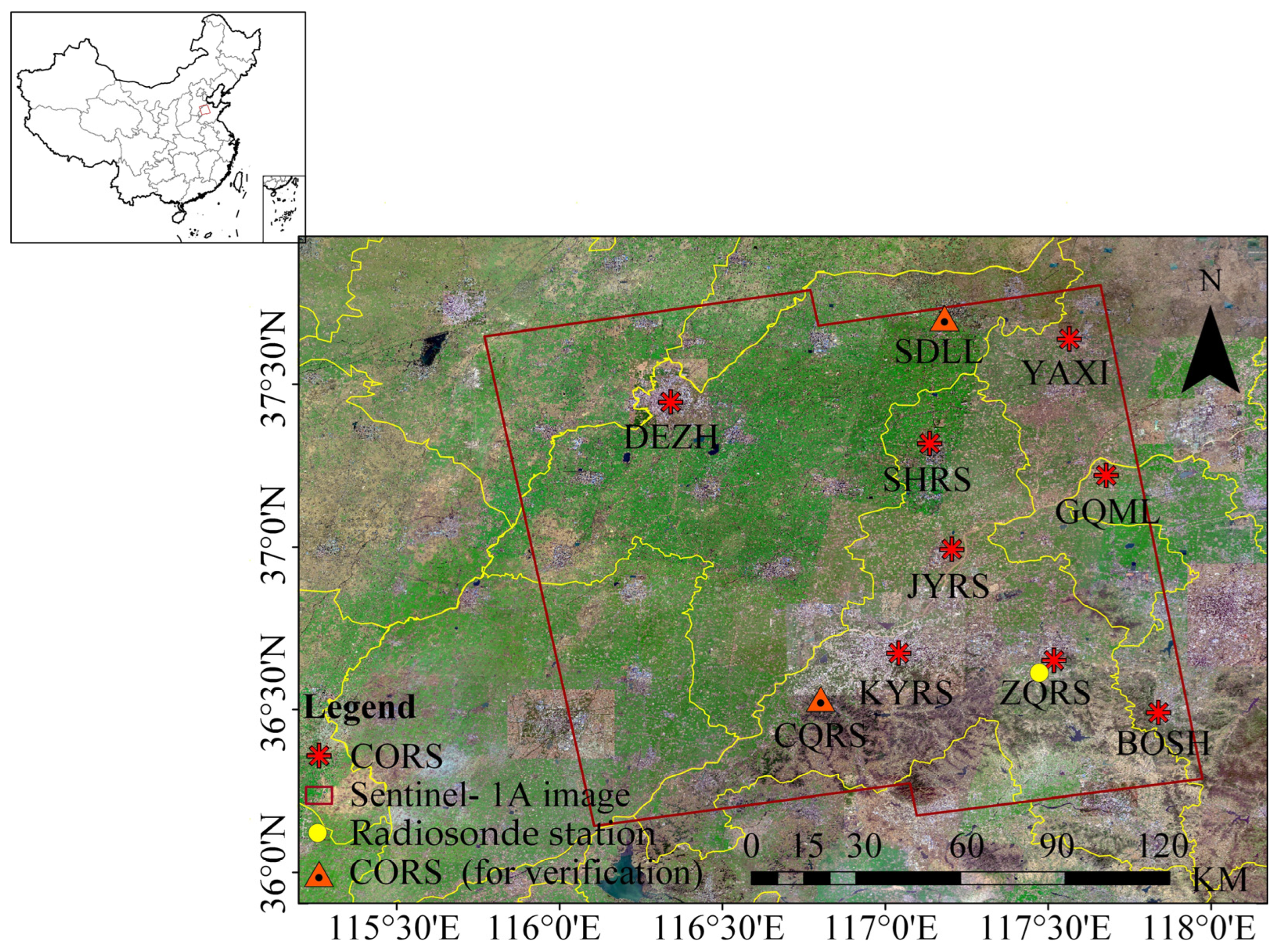
Jinan is the capital of Shandong Province and a supercity in China. This city is located in the eastern region of China, in the central and western part of Shandong Province, on the southeastern edge of the North China Plain. The geographical coordinates of Jinan are 114°–119° E and 35°–38° N. The elevation of this area is 0–1500 m. Jinan’s topography features a south-to-north, high-to-low gradient. The region includes mountains, hills, and the Yellow River alluvial plain. The region belongs to the warm temperate continental monsoon climate zone, characterized by distinct monsoons and well-defined four seasons. In spring, the area experiences hydrostatic and less rainy conditions. Summer is characterized by warm temperatures and abundant rainfall. Autumn is cool and dry, while winter is cold with little snowfall. The Bohai Sea is situated in the northeast direction of Jinan, contributing to the abundant atmospheric water vapor content in the region. At the same time, the region has BDS observations from 10 Continuous Operational Reference System stations (CORS) provided by the Shandong Provincial Institute of Land and Resources Surveying and Mapping, which is suitable for the research of InSAR-derived PWV. The red dots in Figure 1 represent the spatial distribution of CORS stations.
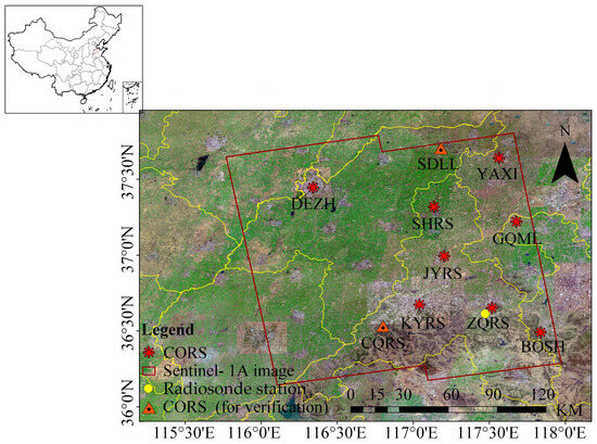
Figure 1.
Study area overview.
A total of 29 Sentinel-1A images were selected for PWV retrieval. These images spanned from 2020, covering the geographical area of Jinan and its surrounding regions. The relevant data parameters, providing essential information about the dataset, are comprehensively presented in Table 1.

Table 1.
Sentinel-1A data overview.
In order to mitigate the effects of surface deformation and temporal incoherence on the retrieval of PWV, a time baseline threshold of 24 days and a spatial baseline threshold of 130 m were set for the interferogram combination. This selection was based on the understanding that surface deformation typically does not occur significantly within 24 days. Under these criteria, a total of 20 interferograms were generated for this experiment. To further enhance the accuracy of the analysis, the US Space Shuttle Radar Mapping Program (SRTM-DEM) was utilized to remove the topographic phase, and The POD Precise Orbit Ephemerides was employed to correct satellite orbit errors. The spatial resolution of SRTM-DEM is 30 m. The POD Precise Orbit Ephemerides is the most accurate orbital data. These data are released with a delay of 26 days. Its positioning accuracy is better than 5 cm. The time–space baselines of the InSAR interferograms are presented in Table 2.
Table 2.
Time–space baseline of the interferograms.
The BDS observations provided by the Shandong CORS were utilized in the process of retrieving PWV. The time resolution of the BDS observational data is 30 s. We utilized the BDS observations from 10 CORS stations (SDLL, YAXI, DEZH, SHRS, GQML, JYRS, KYRS, ZQRS, CQRS, and BOSH). The calculation process of BDS PWV involved the utilization of BDS observation files (O-files), navigation files (C-files), precise ephemeris files (SP3-files), etc. The O-files provide essential information of range codes and carrier phase data from BDS. The N-files provide crucial broadcast ephemeris, operational status, and time information of BDS. The SP3-files, provided by the IGS Analysis Center of Wuhan University, was used for positioning the precise orbit of BDS.
ERA5 is the fifth-generation atmospheric reanalysis data for global climate produced by ECMWF. It is based on the 4-dimensional variational assimilation of global surface and satellite meteorological data [39]. This study utilized temperature, relative humidity, and geopotential data of ERA5 to calculate the weighted mean temperature Tm. They had a temporal resolution of 1 h, a horizontal resolution of 0.25° × 0.25°, and a vertical resolution spanning 37 pressure levels, respectively. We also utilized the surface pressure data of ERA5 to calculate the hydrostatic delay.
2.2. Methodology
Aimed at retrieving PWV from the atmosphere phase screen of InSAR, this paper had an optimized framework. In Section 2.2.1, the retrieval of zenith wet delay from the SAR interferogram is described. We innovatively compared the accuracy of the hydrostatic delay between GNSS and the calculation results by ERA5 data and put forward the threshold value of the hydrostatic delay deviation. Section 2.2.2 describes the method for computing the water vapor conversion factor by using ERA5 data. We applied an integration method to use ERA5 data, including relative humidity, temperature, and geopotential, to calculate the weighted average temperature. Additionally, the principle of calibration using BDS observations is described. Figure 2 shows the new framework in detail.
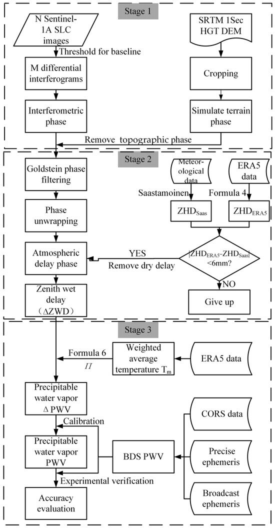
Figure 2.
Retrieval flowchart of InSAR PWV. П represents the water vapor conversion factor.
First, the small baseline subset of differential interferometry (SBAS) was used to generate interferograms [40,41,42,43]. The time baseline threshold was set to be less than or equal to 24 days. The spatial baseline threshold was set to be less than 130 m. In this process, the SRTM-DEM were used to remove the topographic phase from the interferograms. The precise orbit files were used to remove orbit errors.
Second, the wet delay phase was extracted from the unwrapping phase. After the previous step, the unwrapping phase contains both the hydrostatic delay phase and the wet delay phase. Obtaining the wet delay phase requires accurately calculating and removing the hydrostatic delay phase from the interferograms. In this study, ERA5 data were used to calculate the hydrostatic delay phase. In the process of retrieving BDS PWV, the Saastamoinen model was used to calculate the hydrostatic delay. To minimize their differences, we computed the deviations, and discarded the results with the deviations greater than 6 mm. If the deviation of hydrostatic delay exceeds 6 mm, it will result in a 1 mm deviation on PWV.
Third, the wet delay was converted into PWV. The water vapor conversion factor is an important parameter in this process. We calculated the weighted average temperature for the Jinan area using ERA5 data. To validate its accuracy, we compared it with the weighted average temperature from the radiosonde station. To covert the InSAR ∆PWV to PWV, we used BDS observations for the calibration process.
Finally, we used BDS PWV and ERA5 PWV to validate the accuracy of InSAR PWV. According to results of InSAR PWV, we analyzed the spatio-temporal distribution of PWV in the Jinan area.
2.2.1. Zenith Wet Delay in InSAR Interferograms
The troposphere refractive index depends on the water vapor content, pressure, and temperature variations, influencing the velocity of the electromagnetic signals. According to atmospheric structure, if we neglect other minor atmospheric constituents with a negligible impact, the refractivity N can generally be decomposed into: hydrostatic, wet, ionospheric, and liquid water refractivity. The total refractive index of electromagnetic signals affected by the atmosphere can be represented as:
where N is the refractivity. Nhyd, Nwet, Nion, and Nliq present the hydrostatic, wet, ionospheric and liquid water refractivity, respectively. k1 = 77.689 KhPa−1, k2 = 71.2952 KhPa−1, and k3 = 3.75463 × 10⁵ K2hPa−1 are called refractivity constants; Pd, T, and e are, respectively, the pressure due to the dry air (in hPa), the temperature (in kelvins), and the water vapor pressure (in hPa); W is the liquid water content (in gm3); ne is the electron density per cubic meter; and f is the radar frequency.
To obtain the phase of wet delay from InSAR interferograms, the SBAS was employed to process the InSAR data. The SBAS combines all SAR images by setting specific spatio-temporal baselines to obtain a set of shorter spatio-temporal baselines. It can overcome the problem of incoherence occurring in differential interferometric synthetic aperture radar (DInSAR). The original N SAR images covering a specific area generate M interferograms by assuming the spatio-temporal baseline within a particular range. This approach optimizes the quality and accuracy of the interferograms. The phase of the (x, y) pixel in the interferogram can be expressed as:
where ti and tj are the acquisition instants of ith and jth SAR image, respectively. is the topographic phase. is the ground deformation phase. is the orbital error phase. is the atmospheric delay phase. is the other noise phases. If there is no deformation on the ground in the study area or the deformation is known, the deformation phase in the interferogram can be removed. The delay phase caused by noise can be eliminated through filtering. According to the theory of atmospheric stratification, the atmospheric delay phase includes ionospheric delay and tropospheric delay. Ionospheric delay has a more significant impact on the radar signal in the longer band and high latitude areas, while it can be ignored for the C band radar signal in this experimental area [44]. In most weather conditions, the delay caused by liquid water is less than 1 mm. Therefore, the delay from liquid water can also be disregarded. Then, Formula (2) can be expressed as:
where represents the differential atmospheric delay phase. is the noise phase. is the tropospheric delay phase. is the hydrostatic delay phase in the troposphere. is the wet delay phase in the troposphere. The atmospheric delay present in the interferogram can be interpreted as the tropospheric delay. PWV is related to the wet delay in the troposphere and has no relationship with the hydrostatic delay. Hence, it is necessary to separate the troposphere wet delay and the troposphere hydrostatic delay. The hydrostatic delay phase can be simulated and calculated using atmospheric parameters, and its expression is [45,46]:
where λ represents the radar wavelength, θ represents the incident angle of the radar signal, K1 represents a physical quantity related to refraction, R is the universal index of ideal gas, g represents gravitational acceleration, Md is the molar mass of hydrostatic air, Pt represents the surface pressure at the imaging time of the slave image, and Pt0 represents the surface pressure at the imaging time of the master image.
The wet delay phase can be obtained by subtracting the hydrostatic delay phase from the total tropospheric delay phase. The zenith wet delay ∆ZWDInSAR can be expressed as [47]:
where λ represents the radar wavelength, θ represents the incident angle of the radar signal, represents the wet delay phase in the radar line-of-sight direction, and ∆ZWDInSAR represents the wet delay in the zenith direction.
2.2.2. Conversion of ZWD into PWV
InSAR ∆PWV was converted from the zenith wet delay, and its expression is [48,49,50]:
where Π is the water vapor conversion factor, which is a dimensionless scaling factor; ρ = 1000 kgm−3; Rv = 461.95 Jkg−1K−1; k3 = 3.75 103 K2Pa−1; and = 0.233 KPa−1. Tm represents the weighted average temperature. Tm is typically calculated using the Bevis empirical model. However, the Bevis empirical model is not suitable for this study area. Therefore, we utilized ERA5 data based on pressure layers (temperature, geopotential, and relative humidity) to calculate Tm. The formula for calculating Tm is as follows [51]:
where Tm represents the weighted average temperature, e represents the partial pressure of water vapor, and T represents the temperature (in K).
The process of phase unwrapping introduces an arbitrary constant. To address this issue, according to Equation (8), InSAR ΔPWV is calibrated by BDS ΔPWV. BDS alone can be used for PWV estimation with an accuracy consistent with GPS [52]. It can be used for this study. It should be noted that the signals from satellites with elevation angles larger than the cut-off elevation angle 15° are recorded by the BDS receiver. Hence, the PWV estimates obtained from BDS were determined by applying the appropriate weighting factors based on the elevation and azimuth angles of the specific ray paths connecting the BDS satellites and the receiver [53].
where NBDS is the number of CORS stations. Np(H) is the number of InSAR pixels within a certain radius circle centered on the H-th CORS station. is the difference in PWV of BDS at the time of acquiring two SAR images, and is the InSAR ∆PWV. In this study, a cut-off angle of θcut = 15° was employed. It was assumed that the atmospheric water vapor is concentrated below 1.4 km in the troposphere. As a result, the radius of the circular region formed by the BDS observation cone is 5.2 km. In the calibration process, it is essential to synchronize Sentinel-1 observation data and BDS observation data in both the temporal and spatial dimensions. Temporally, the average of BDS PWV at 10:10 UTC and BDS PWV at 10:15 UTC was used to represent BDS PWV at 10:13 UTC. Spatially, the average of all pixels within the circular area of the InSAR observation data corresponded to BDS PWV at 10:13 UTC.
It should be noted that this study used the BDS wet delay to spatially calibrate the InSAR wet delay, ensuring the spatial consistency between InSAR ∆PWV and BDS ∆PWV. Then, the Kriging interpolation method was used to interpolate the BDS PWV in order to obtain the PWV spatial distribution map corresponding to the imaging time of the master images [54]. Finally, the BDS PWV spatial distribution map was used to calibrate InSAR ΔPWV in order to retrieve the PWV spatial distribution map in the imaging time of the slave images.
3. Results
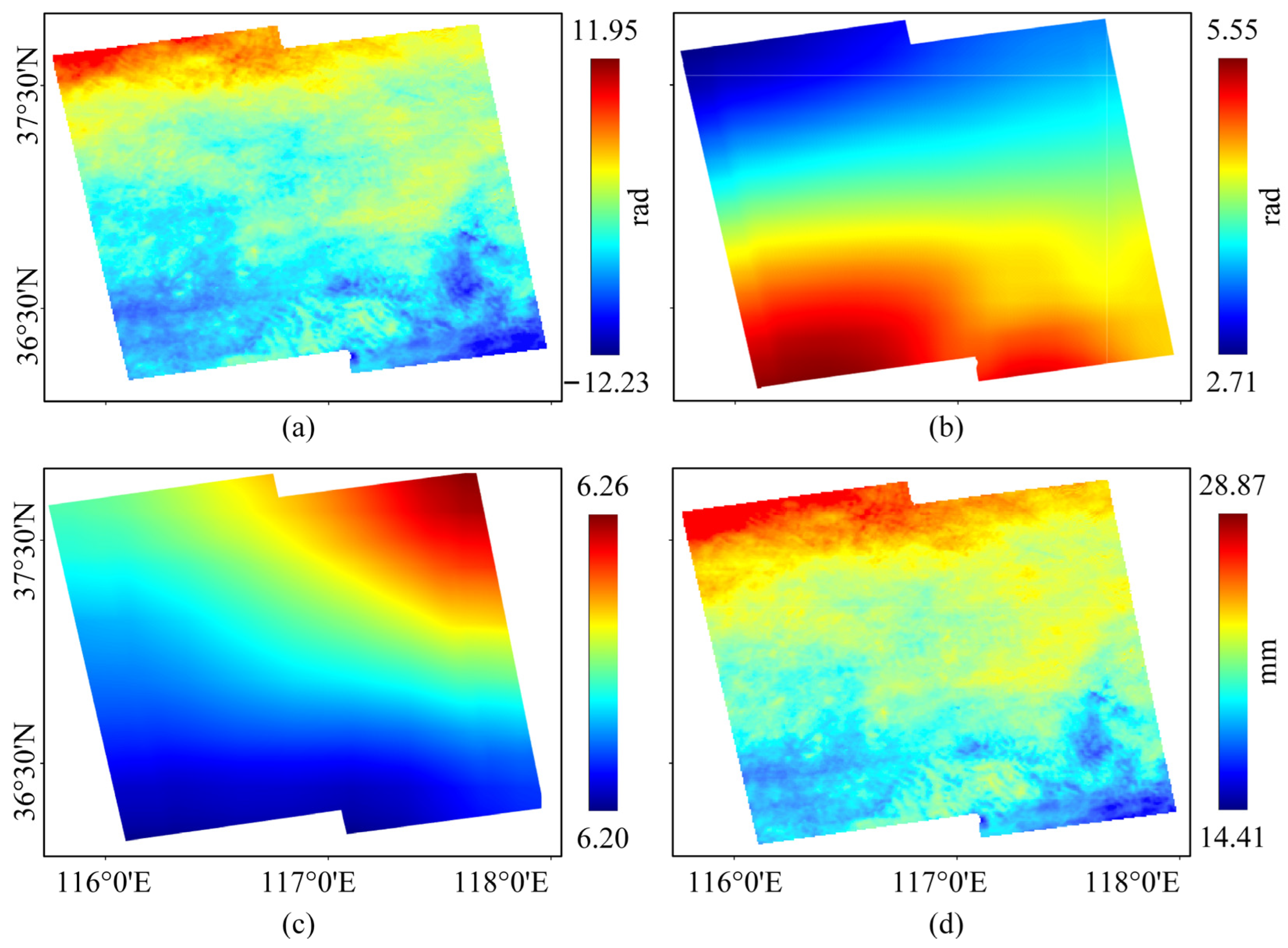
In this study, the tropospheric delay shown in Figure 3a corresponds to interferogram-6. The calculation results of the hydrostatic delay by using ERA5 data (including surface pressure) are shown in Figure 3b. The wet delay was obtained by subtracting the hydrostatic delay from the tropospheric delay. Converting the wet delay to PWV requires the water vapor conversion factor П. It is a dimensionless quantity. In many studies, it is often assumed to be a constant. However, in reality, П is influenced by the weighted average temperature and exhibits temporal and spatial variations. In different seasons of the same region, there will be variations in П in response to Tm. The calculation results of the spatially continuous П by using ERA5 data (including pressure, temperature, and relative humidity) are shown in Figure 3c. It displays the spatial distribution of П in May 2020. To reduce errors, this study employed a weighted average of the water vapor conversion factors corresponding to the master image and the slave image. Then, according to Equation (6), the wet delay was converted to PWV. InSAR ΔPWV was obtained by utilizing BDS observations from eight CORS for the calibration process. Figure 3d shows the distribution map of InSAR ΔPWV on 4 May 2020.
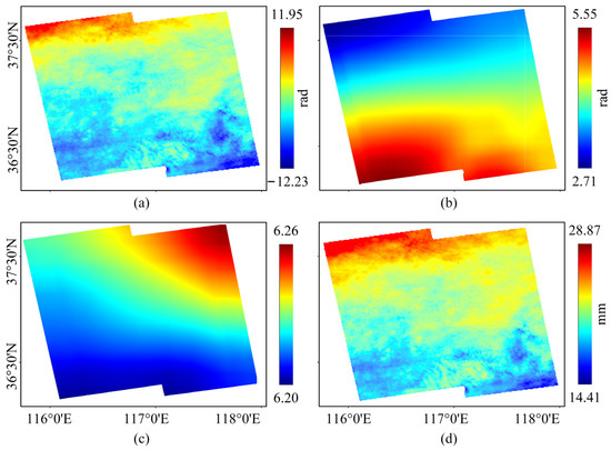
Figure 3.
(a) Total tropospheric delay from the InSAR interferogram. (b) Slant hydrostatic delay difference maps predicted from the ERA5 (taking differential interferogram-6 (master image from 22 April 2020; slave image from 4 May 2020) as an example). (c) The spatial distribution of the conversion factor П calculated based on ERA5. It was calculated at the time 10:00 UTC (the imaging time corresponding to Sentinel-1A). (d) The ΔPWV distribution map on 4 May 2020.
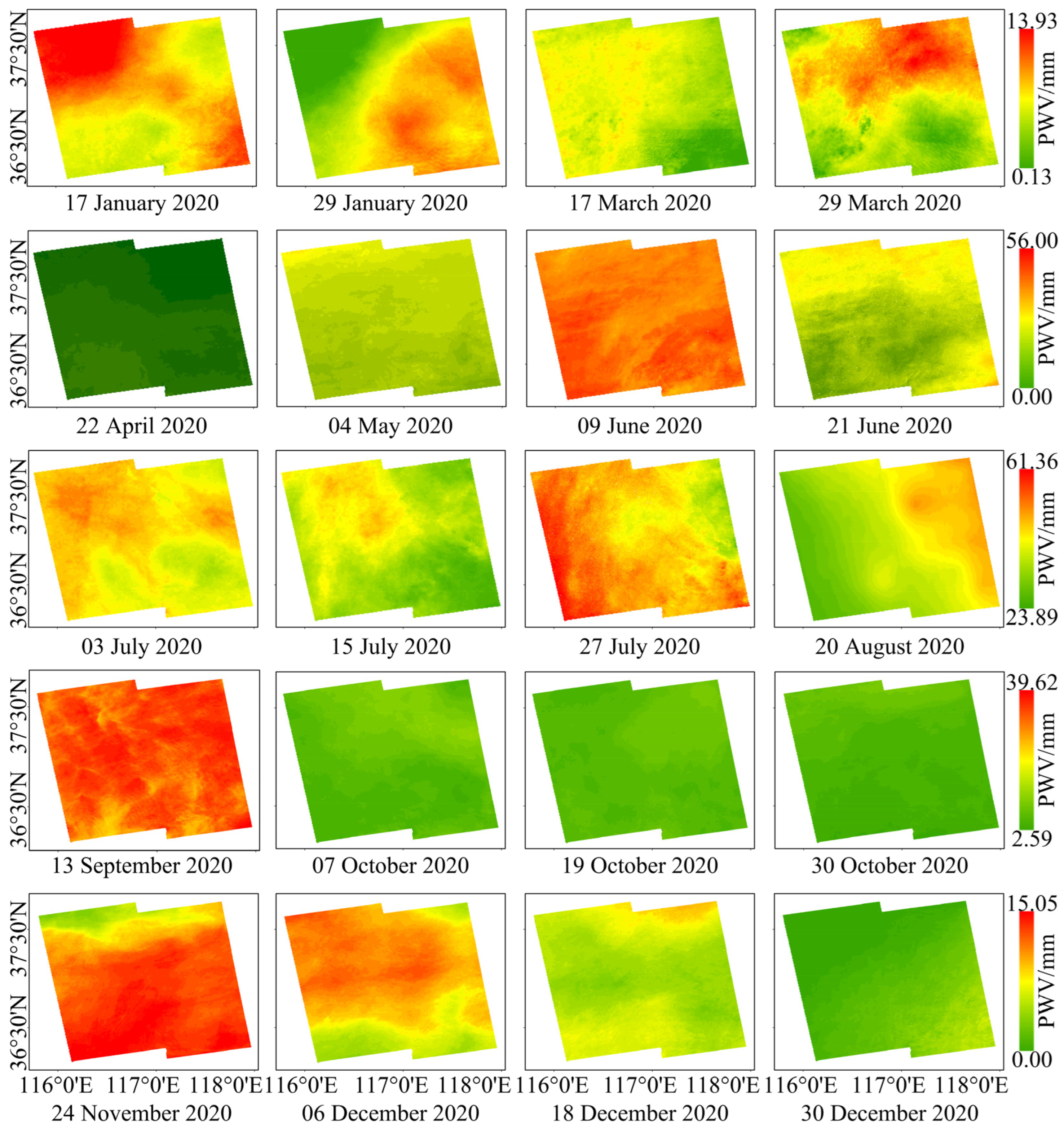
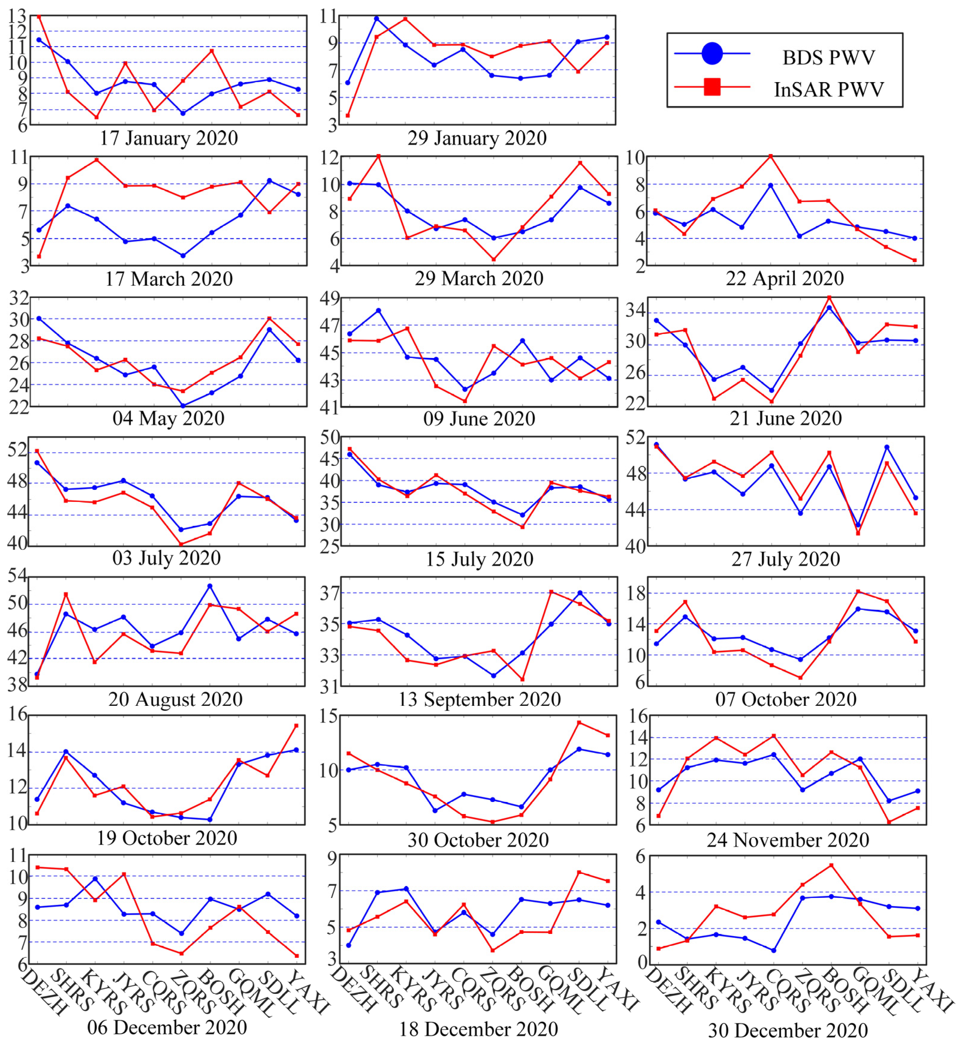
The BDS PWV was interpolated using the Kriging method to generate the PWV distribution map corresponding to the master image (BDS PWV distribution map). Subsequently, the BDS PWV distribution map was added to the InSAR ∆PWV to obtain the InSAR PWV distribution map (Figure 4). It can be seen that using InSAR to retrieve PWV can reflect both the spatial changes in PWV in a large area and the changes in PWV within a small area. It is evident that PWV values are lower during the spring and winter seasons, and higher during the summer and autumn seasons. This phenomenon may be attributed to the temperate monsoon climate prevalent in the region. In such a climate, the winter experiences scarce rainfall and dry weather, while the summer receives more rainfall and humid weather. We were able to identify not only the temporal distribution characteristics of PWV but also the spatial distribution features of PWV. The spatial distribution of PWV can be roughly categorized into three types. The first type is characterized by uniformly high values of PWV. The second type exhibits generally low values of PWV. The third type shows an irregular spatial distribution of PWV. In Figure 4, the dates 9 June 2020, 13 September 2020, and 24 November 2020 fall into the first category. The dates 22 April 2020, 4 May 2020, 7 October 2020, 19 October 2020, 31 October 2020, and 30 December 2020 fall into the second category. The remaining dates in Figure 4 belong to the third category.
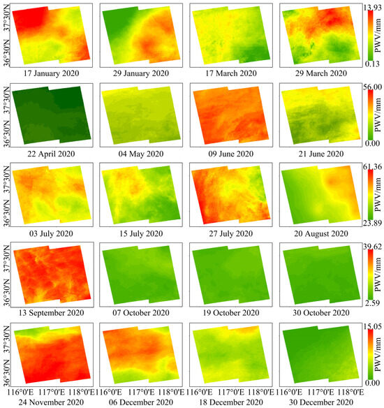
Figure 4.
Results of using InSAR to retrieve PWV.
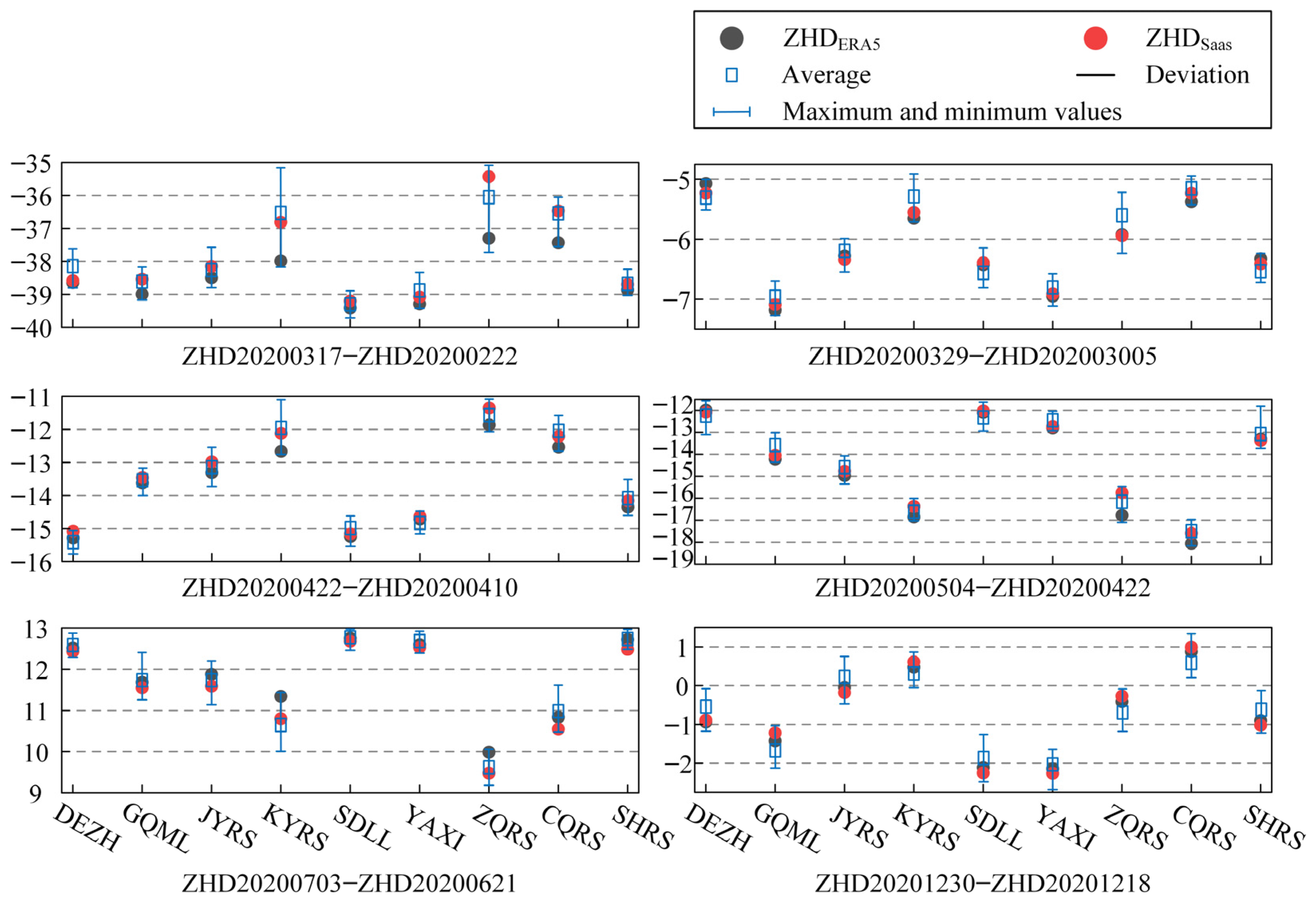
In this study, the InSAR hydrostatic delay calculation model was utilized to simulate the hydrostatic delay phase in the interferograms (ZHDERA5). BDS employs the Saastamoinen model to calculate the zenith hydrostatic delay (ZHDSaas). These two models exhibit differences and thus necessitating an analysis of the disparities in the hydrostatic delays.
We examined the hydrostatic delays from nine CORS stations across six InSAR interferograms (as depicted in Figure 5). The results reveal a high correlation coefficient (r) of 0.99 between the two types of zenith hydrostatic delays; the RMSE was 0.05 mm and the mean absolute error (MAE) was 0.29 mm. Notably, the deviations between the two types of hydrostatic delays were negligible. The differences between the two models in calculating hydrostatic delays resulted in PWV discrepancies of less than 0.04 mm. Consequently, the errors from variations in the zenith hydrostatic delay models can be disregarded during the PWV calculation process. In this investigation, all the deviations were less than 2 mm. Deviations greater than 1 mm accounted for 5.5% of the total, whereas those less than 0.29 mm constituted 75.9%. These suggest that, even if the two models have a little difference, there may be a degree of uncertainty present in the results of the hydrostatic delay.
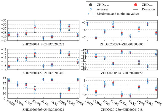
Figure 5.
Comparison between the hydrostatic delay from the Saastamoinen model and the hydrostatic delay from ERA5. The squares indicate ZHD estimates from ERA5 data that are obtained by averaging all pixels falling within the circular area with a radius of 5.2 km centered around the station, corresponding to the observational data.
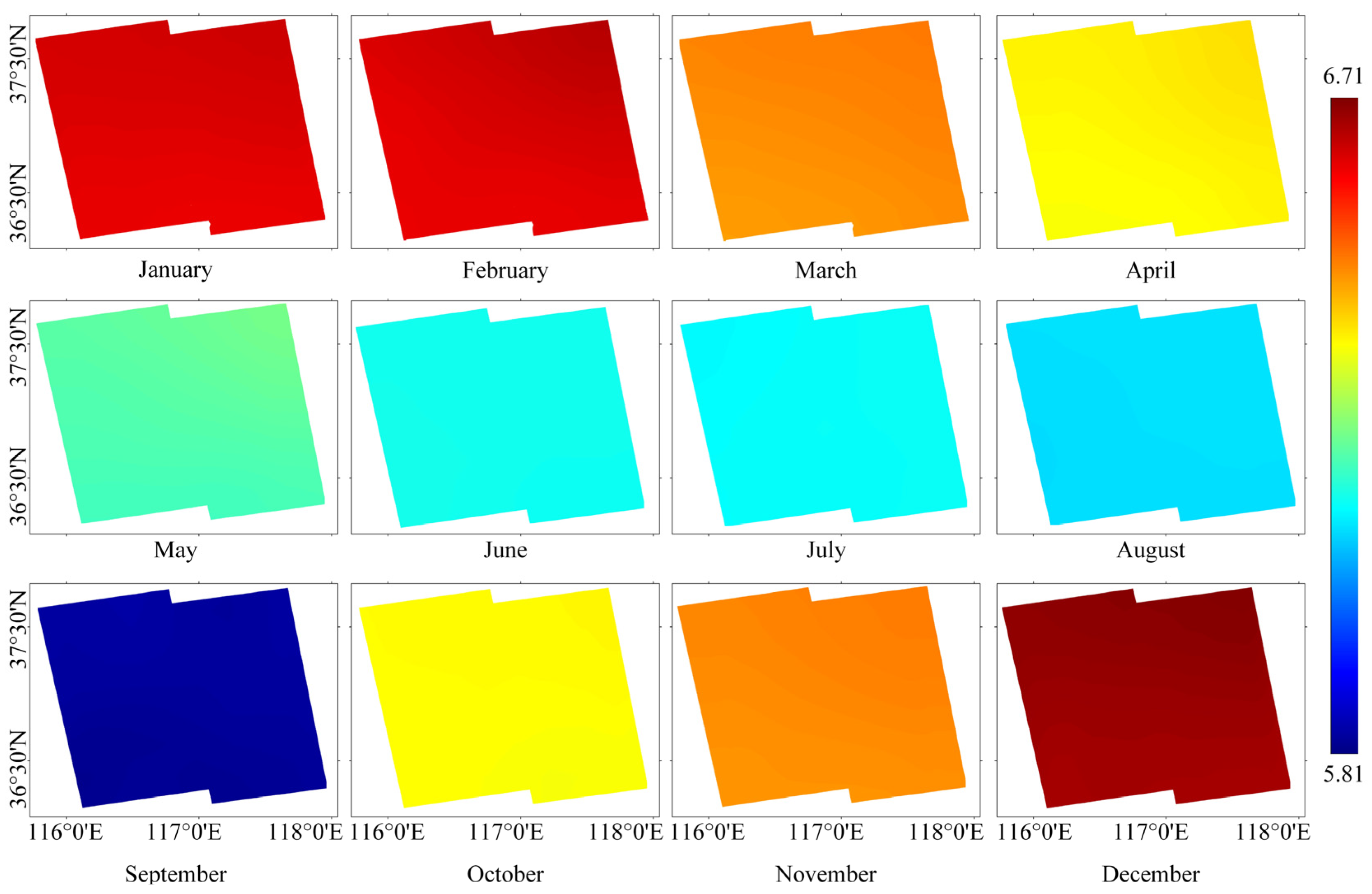
In general, the water vapor conversion factor П is treated as a constant based on the empirical model. However, П depends on mean temperature profiles, varying with season, weather, and specific location, which induces the value of П to vary by as much as 10% [55]. On account of the spatio-temporal variations in temperature and relative humidity, the water vapor conversion factor П (Figure 6) demonstrates spatio-temporal variations. Hence, it is crucial to accurately obtain the water vapor conversion factor П for each pixel of Sentinel-1A in order to convert ∆ZWD to ∆PWV. We used ERA5 data (relative humidity, temperature, and geopotential) to calculate spatial-continuous П for the Jinan region. In order to standardize the spatial resolution of П and the Sentinel-1A observations, the Kriging interpolation method was employed in this study to ensure consistent resolution between the Sentinel-1A data and П.
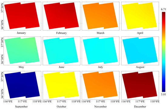
Figure 6.
Water vapor conversion factor П calculated from the ERA5 reanalysis data (The water vapor conversion factor П from January to December are shown in the figure, respectively).
Figure 6 illustrates the spatial distribution of the atmospheric water vapor conversion factor П in the Jinan region. The analysis reveals that П exhibits a high value during the autumn and winter seasons, while it shows a low value during the spring and summer seasons. Moreover, as the temperature increases in the Jinan, there is a gradual decrease in the atmospheric water vapor conversion factor П. It is worth noting that, in Figure 6, the shared color bar among the 12 distribution maps of П makes it challenging to visually discern the precise distribution of П within the figure. It is important to acknowledge that П exhibits spatial variations, as demonstrated in Figure 3c. In 2020, the variation of П in the Jinan ranged from 5.81 to 6.71. The changes in П have exceeded 10%. This work demonstrated that it is not prudent to consider П as a constant in the process of InSAR PWV retrieval.
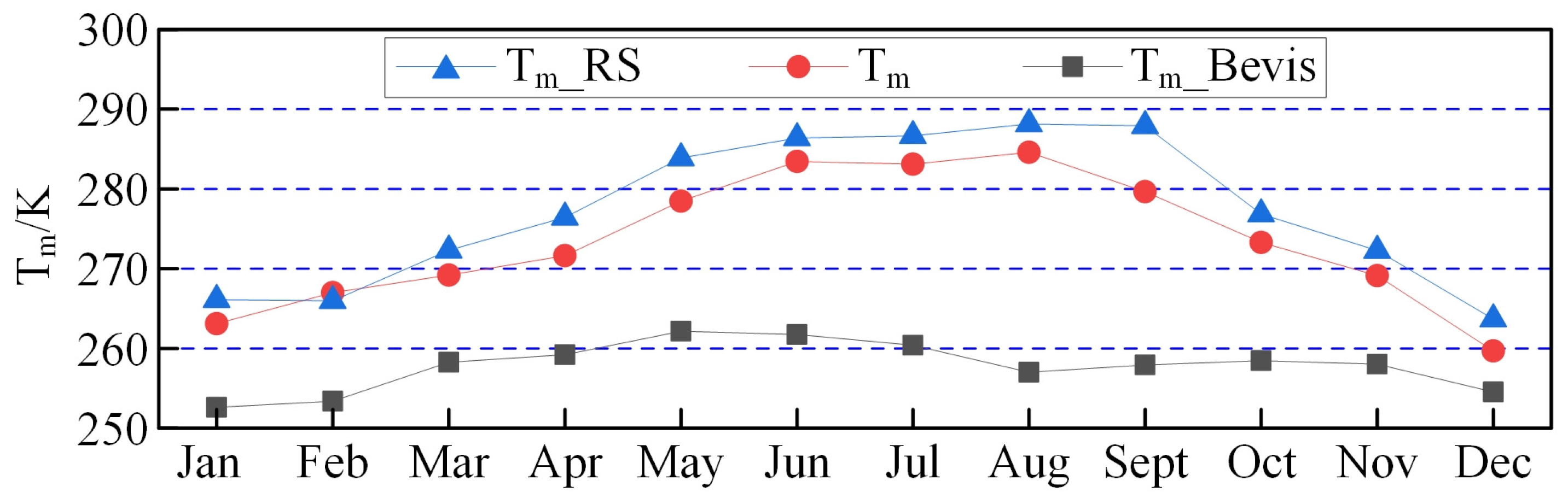
According to Equation (6), it can be seen that П is a function of Tm. The accuracy of П is directly related to the accuracy of Tm. Therefore, this study used an integration method to calculate the Tm for the Jinan area. To validate the accuracy of Tm, the monthly average Tm was calculated using data from a radiosonde station located in Zhangqiu District, Jinan City (Tm_RS). This study also calculated the monthly average Tm using the Bevis empirical model (Tm_Bevis). We compared these three types of Tm. The results show that the average absolute deviation between Tm_Bevis and Tm_RS is 15.7 K. The absolute average deviation between the Tm calculated using the method in this paper and Tm_RS is 3.9 K. Figure 7 illustrates the comparison of the three types Tm.

Figure 7.
Comparison of Tm_RS, Tm_Bevis, and the method for calculating Tm presented in this study.
4. Discussion
To validate the reliability of retrieving InSAR PWV using this method, the accuracy and reliability of the results were verified using the BDS observational data of ten CORS stations in the study area. Eight CORS stations were used for the InSAR calibration process, and the other two CORS stations (CQRS and YAXI) were used as verification stations. CQRS and YAXI did not participate in the PWV retrieval process. Therefore, comparing the BDS PWV of CQRS and YAXI with the InSAR PWV is more convincing. Figure 8 presents a comparison between InSAR PWV and BDS PWV. It reveals a remarkable similarity in their variations with only a slight deviation observed. The analysis indicates that the PWV in the Jinan region exhibits a seasonal characteristic. Its temporal distribution is characterized by lower values during winter and elevated values during summer. From Figure 8, it can be observed that, from January to April 2020, the PWV values in the Jinan area ranged from 2 mm to 13 mm. From May to September 2020, the PWV values in the Jinan area ranged from 22 mm to 54 mm. From October to December 2020, the PWV values in the Jinan area ranged from 0 mm to 18 mm. This phenomenon can be attributed to the prevailing temperate monsoon climate, characterized by hot and rainy summers, and dry and less rainy winters.
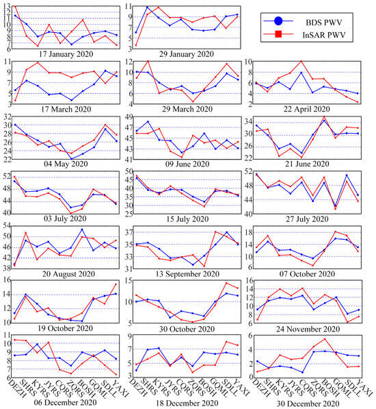
Figure 8.
Comparison of the results of InSAR PWV and BDS PWV (The y-axis represents the PWV in millimeters, while the x-axis denotes CORS, CQRS, and YAXI, which were only included in the validation process).
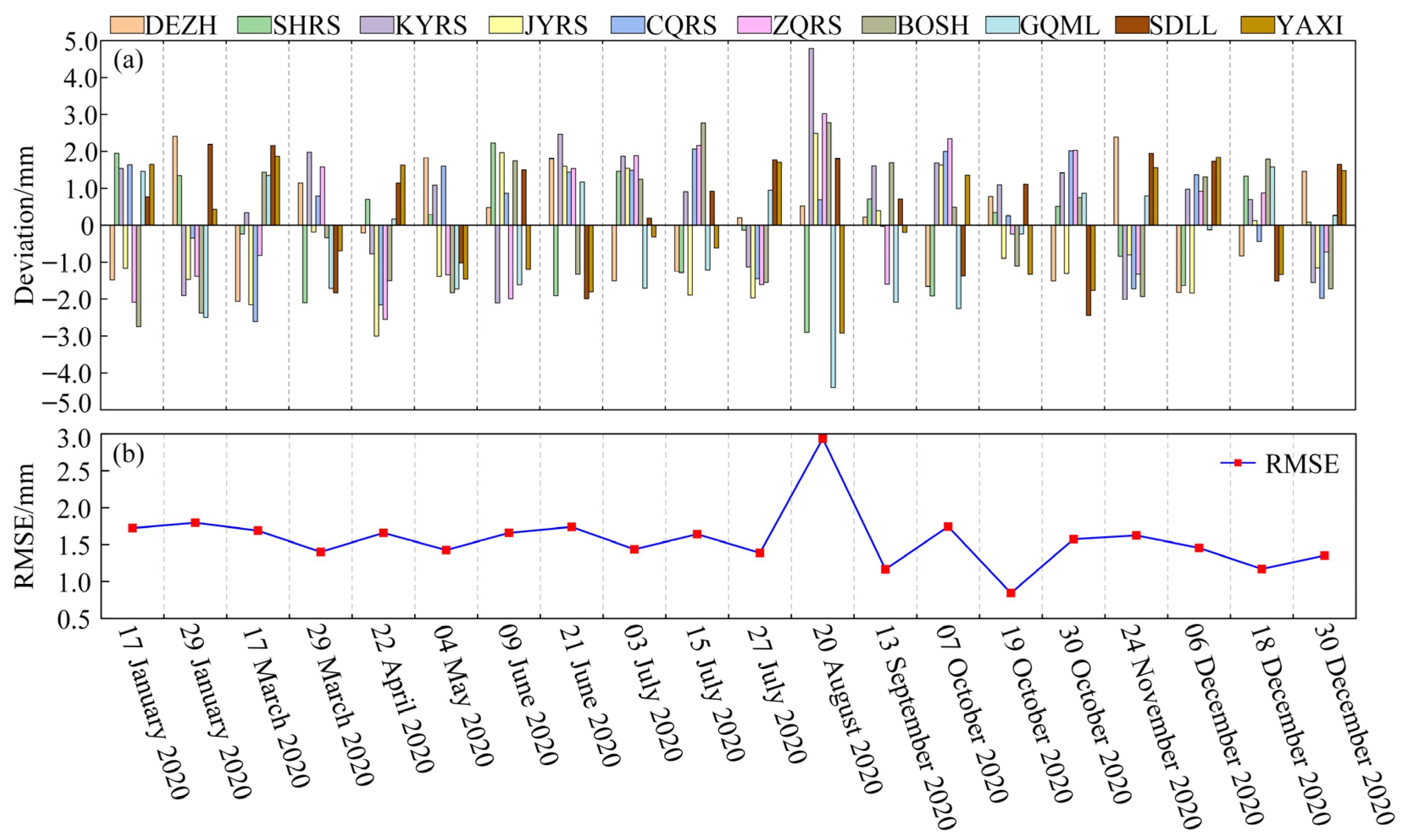
Figure 9 reveals that the average deviation between InSAR PWV and BDS PWV ranges from 0.74 mm to 2.63 mm, with an overall average deviation of less than 2.7 mm. The RMSE is less than 3 mm. The maximum deviation between BDS PWV and InSAR PWV among the two CORS stations used for validation is 2.9 mm and the minimum deviation is 0.19 mm. These two CORS stations exhibit similar results to the other CORS stations, with no significant deviations observed. Notably, the highest values of deviation and RMSE are observed on 20 August 2020. This deviation can be attributed to residual error phases introduced during InSAR data processing, potentially stemming from the utilization of external DEM data and precision track data. For the remaining interferograms, the average deviation remains below 1.8 mm. We calculated the correlation coefficient between InSAR PWV and BDS PWV, which is 0.98. This indicates a strong correlation between them. The BDS PWV has a strong stability. The InSAR PWV have the advantage of spatial continuity.
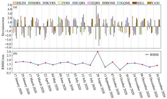
Figure 9.
(a) Deviation between InSAR PWV and BDS PWV (b) RMSE between InSAR PWV and BDS PWV.
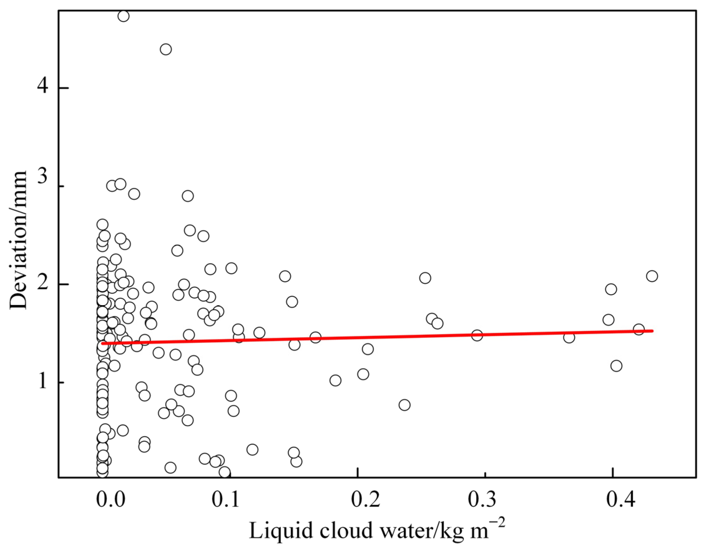
During the data processing, we ignored the influence of liquid cloud water on InSAR. Therefore, we analyzed the correlation between liquid cloud water with the deviation of InSAR PWV and BDS PWV. The correlation coefficient between the deviation and liquid cloud water is 0.034. The results indicate that there is no significant correlation between them. Figure 10 illustrates the correlation between the deviation and liquid cloud water.
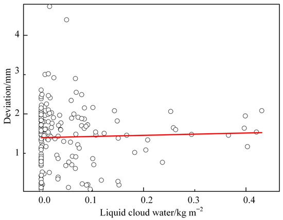
Figure 10.
The correlation between the deviation and liquid cloud water. The circles represent the value of liquid cloud water corresponding to deviation. The red line is the fitted linear function.
The accuracy of InSAR PWV can be verified by comparing with BDS PWV. However, since the BDS observations are discrete point data, it is difficult to describe the characteristics of the spatial distribution of PWV. Hence, we compared InSAR PWV with ERA5 PWV in order to discuss their similarities and differences in spatial distribution.
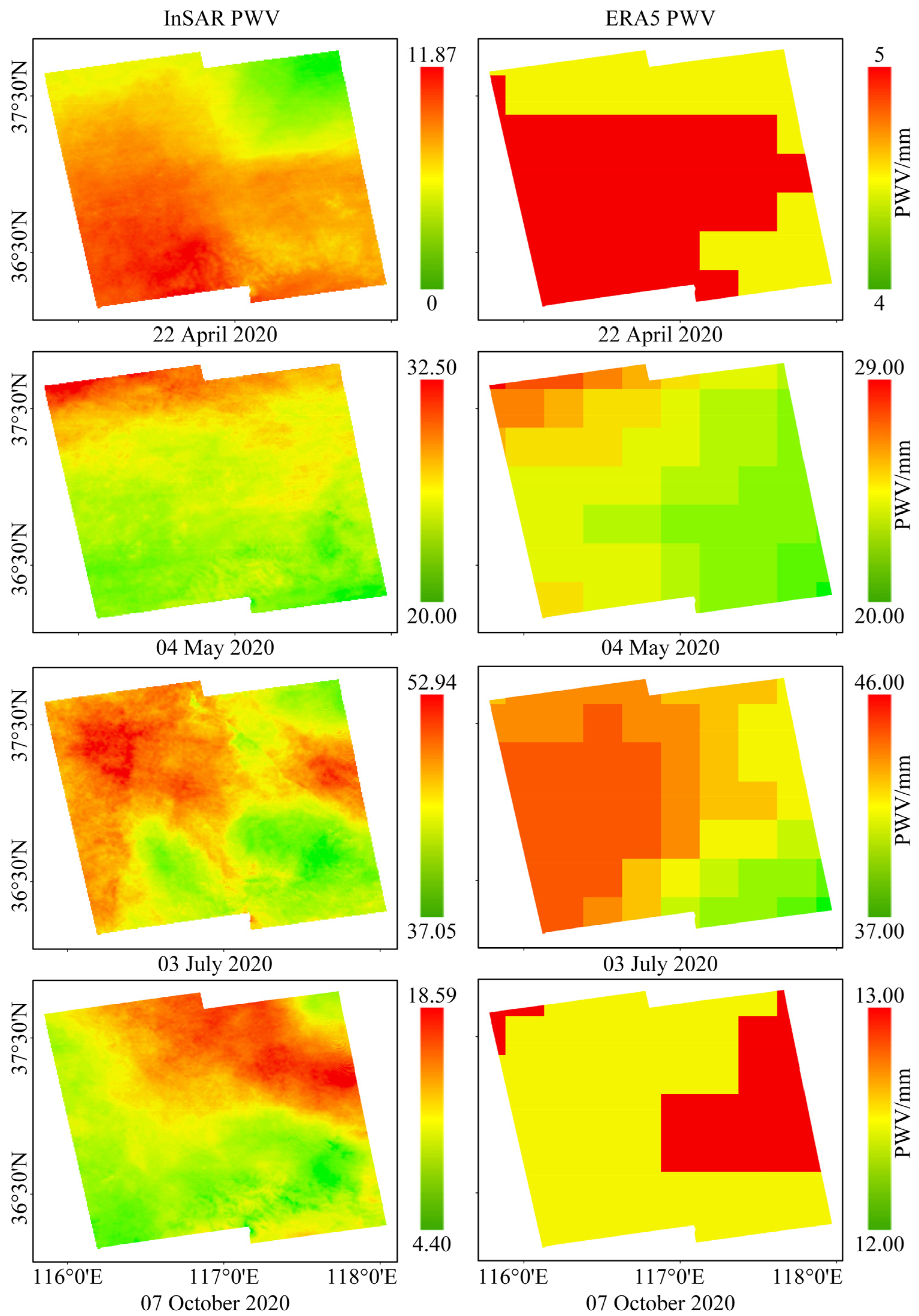
Figure 11 shows the spatial distribution of InSAR PWV and ERA5 PWV on 22 April 2020, 4 May 2020, 3 July 2020, and 7 October 2020. It can be observed that, on 22 April 2020, both InSAR PWV and ERA5 PWV exhibited an increasing trend from the northeast to the southwest. The maximum PWV values were found in the southwest. There is a significant deviation between the values of InSAR PWV and ERA5 PWV. The deviation between their maximum values is 6.87 mm, and the deviation between their minimum values is 4 mm. On 4 May 2020, both InSAR PWV and ERA5 PWV showed a decreasing trend from north to south, with smaller deviations in their PWV values. On 3 July 2020, both InSAR PWV and ERA5 PWV exhibited a decreasing trend from west to east. On 7 October 2020, there was a significant difference in the spatial distribution of InSAR PWV and ERA5 PWV. Among all 20 dates in 2020, the comparison between InSAR PWV and ERA5 PWV shows both consistency and differences. We conducted an analysis to identify the possible reasons for this phenomenon. We believe that it could be attributed to the following factors:
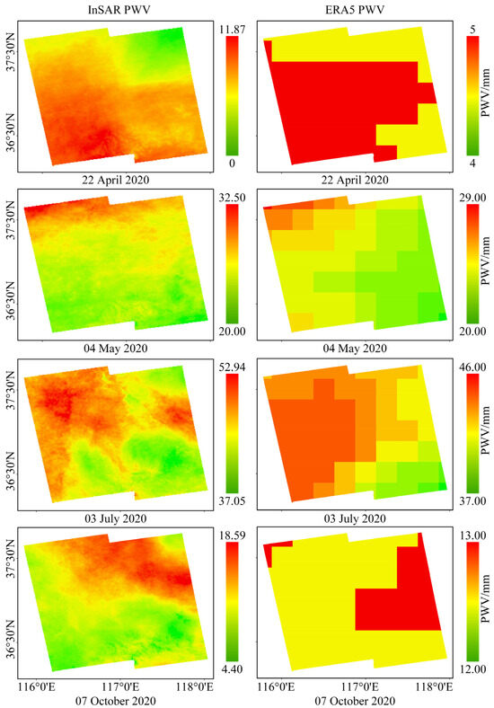
Figure 11.
Comparison between InSAR PWV and ERA5 PWV (The first column is InSAR PWV, and the second column is ERA5 PWV).
- Difference in resolution between InSAR PWV and ERA5 PWV data. Compared to the high resolution of the Sentinel-1A observations, the resolution of ERA5 data (0.25° × 0.25°) is lower. Each pixel of ERA5 data represents the average value of all pixels within the same range of InSAR PWV. This may be one of the reasons for the deviation between ERA5 PWV values and InSAR PWV values.
- ERA5 data assimilate multi-source observation data, such as meteorological stations, microwave radiometer, and satellite remote sensing. In order to achieve a consistent spatial resolution of the data, the data are interpolated onto a global grid. This processing method may introduce errors in the resulting data. This may be one of the reasons for the deviation between ERA5 PWV values and InSAR PWV values.
- The impact of the simulation result of the main image’s acquisition time. During the process of obtaining InSAR PWV, we used the Kriging interpolation to process BDS data from eight CORS and obtained BDS PWV distribution maps corresponding to the main image’s acquisition time. This process may introduce errors. However, as the number of CORS increases, this error is expected to gradually decrease.
Compared to ERA5 PWV, the retrieval of PWV using Sentinel-1A observations exhibited a higher resolution and the accuracy was sufficient to meet the requirements of meteorological research. This is highly encouraging, particularly for the meteorology community, providing crucial information to be assimilated into numerical weather models and potentially improve forecasts.
5. Conclusions
This study proposed an optimized framework for PWV mapping using TS-InSAR and GNSS. In order to improve the quality of maps of PWV, the hydrostatic delay was precisely estimated by using ERA5 data. We also used the ERA5 data to produce maps of the conversion factor for mapping the zenith wet delay onto PWV at each pixel in the radar scene. The conclusions are as follows:
- In this study, we used BDS observations for calibration processing. This method can solve the problem of a lack of synchronous observations when retrieving non-differential PWV using Sentinel-1A satellite observations. To validate the consistency between ZHDERA5 and ZHDSaas, we calculated their deviations and analyzed their correlation. The results indicate that the deviations between them are small. In the data processing stage, if their deviation exceeds 6 mm, this dataset is excluded. If the deviation of hydrostatic delay exceeds 6 mm, it will result in a deviation of 1 mm on PWV.
- We used ERA5 data to calculate Tm to obtain the water vapor conversion factor. Using Tm-RS as the reference, the Tm in this study was more precise than Tm-Bevis. The PWV retrieval by this method was spatially continuous, which is beneficial for the study of PWV spatial features. The InSAR PWV has a strong consistency with BDS PWV. Using BDS PWV as a reference value, the average deviation of InSAR PWV is between 0.74 mm and 2.63 mm.
- The PWV distribution map obtained using high-resolution observation data can effectively reflect the local details of PWV. This study retrieved the PWV distribution map of Jinan in 2020. The results of this study can reflect the seasonal changes in PWV in the Jinan region. This has reference value for studying the distribution of PWV in the Jinan region.
In conclusion, we verified the reliability of the optimized framework for PWV mapping using TS-InSAR and GNSS. The accuracy of the PWV retrieved using this method meets the requirements of meteorological research and can provide a reference for studying the distribution of PWV. The PWV distribution map obtained using Sentinel-1A observations has a high spatial resolution, which can provide data support for other meteorological models.
Author Contributions
Conceptualization, Q.G., D.L., M.Y. and S.H.; methodology, Q.G., D.L. and M.Y.; software, M.Y.; validation, Q.G. and D.L.; formal analysis, Q.G., D.L. and M.Y.; investigation, Q.G. and D.L.; resources, Q.G., D.L. and Y.S.; data curation, M.Y. and X.X.; writing—original draft preparation, Q.G., M.Y. and D.L.; writing—review and editing, Q.G., D.L. and M.Y.; visualization, M.Y.; supervision, Q.G., D.L., Y.S. and C.Z.; project administration, Q.G., D.L. and Y.S.; funding acquisition, Q.G. and D.L. All authors have read and agreed to the published version of the manuscript.
Funding
This work was supported by the Shandong Provincial Natural Science Foundation, China (ZR2021QD155, ZR2017MD029, and ZR2022MD103); in part by the Natural Science Foundation of China (General Program) (42374049); and in part by the State Key Laboratory of Geodesy and Earth’s Dynamics (Institute of Geodesy and Geophysics, CAS) under the grant (SKLGED2021-5-5).
Institutional Review Board Statement
Not applicable.
Informed Consent Statement
Not applicable.
Data Availability Statement
The BDS observation data are confidential. The data presented in this study are available on request from the corresponding author.
Acknowledgments
The authors are grateful to the European Space Agency (ESA) for free access to the Sentinel-1A satellite data. Also, we would like to thank the Shandong Provincial Institute of Land Surveying and mapping for providing CORS data. We would like to thank the European Centre for Medium-range Weather Forecast (ECMWF) for providing the atmospheric data (ERA5). The authors are grateful for the support from Academician Zhou Chenghu’s team, Shandong Jianzhu University. The authors greatly appreciate the editors and the anonymous reviewers of this manuscript.
Conflicts of Interest
The authors declare no conflict of interest.
References
- Manandhar, S.; Lee, Y.H.; Meng, Y.S.; Yuan, F.; Ong, J.T. GPS-Derived PWV for Rainfall Nowcasting in Tropical Region. IEEE Trans. Geosci. Remote Sens. 2018, 56, 4835–4844. [Google Scholar] [CrossRef]
- Liang, H.; Cao, Y.; Wan, X.; Xu, Z.; Wang, H.; Hu, H. Meteorological applications of precipitable water vapor measurements retrieved by the national GNSS network of China. Geod. Geodyn. 2015, 6, 135–142. [Google Scholar] [CrossRef]
- Nina, A.; Radović, J.; Nico, G.; Popović, L.Č.; Radovanović, M.; Biagi, P.F.; Vinković, D. The Influence of Solar X-ray Flares on SAR Meteorology: The Determination of the Wet Component of the Tropospheric Phase Delay and Precipitable Water Vapor. Remote Sens. 2021, 13, 2609–2626. [Google Scholar] [CrossRef]
- Liu, H.; Huang, S.; Xie, C.; Tian, B.; Chen, M.; Chang, Z. Monitoring Roadbed Stability in Permafrost Area of Qinghai–Tibet Railway by MT-InSAR Technology. Land 2023, 12, 474–492. [Google Scholar] [CrossRef]
- Pezzo, G.; Palano, M.; Beccaro, L.; Tolomei, C.; Albano, M.; Atzori, S.; Chiarabba, C. Coupling Flank Collapse and Magma Dynamics on Stratovolcanoes: The Mt. Etna Example from InSAR and GNSS Observations. Remote Sens. 2023, 15, 847–863. [Google Scholar] [CrossRef]
- Niu, C.; Yin, W.; Xue, W.; Sui, Y.; Xun, X.; Zhou, X.; Zhang, S.; Xue, Y. Multi-Window Identification of Landslide Hazards Based on InSAR Technology and Factors Predisposing to Disasters. Land 2023, 12, 173–187. [Google Scholar] [CrossRef]
- Awasthi, S.; Varade, D.; Bhattacharjee, S.; Singh, H.; Shahab, S.; Jain, K. Assessment of Land Deformation and the Associated Causes along a Rapidly Developing Himalayan Foothill Region Using Multi-Temporal Sentinel-1 SAR Datasets. Land 2022, 11, 2009–2029. [Google Scholar] [CrossRef]
- Liao, M.; Lin, H. Synthetlc Aperture Radar Interferometry Principle and Signal Processing, 1st ed.; Surveying and Mapping Publishing House: Beijing, China, 2003; pp. 84–103. [Google Scholar]
- Hu, J.; Li, Z.W.; Li, J.; Lei, Z.; Ding, X.L.; Zhu, J.J.; Qian, S. 3-D movement mapping of the alpine glacier in Qinghai-Tibetan Plateau by integrating D-InSAR, MAI and Offset-Tracking: Case study of the Dongkemadi Glacier. Glob. Planet. Chang. 2014, 118, 62–68. [Google Scholar] [CrossRef]
- Ge, D. Research on the Key Techniques of SAR Interferometry for Regional L Subsidence Monitoring. Ph.D. Thesis, China University of Geosciences, Beijing, China, 2013. [Google Scholar]
- Zhu, J.; Li, Z.; Hu, J. Research Progress and Methods of InSAR for Deformation Monitoring. J. Geod. Geoinf. Sci. 2017, 46, 1717–1733. [Google Scholar]
- Li, S.; Xu, W.; Li, Z. Review of the SBAS InSAR Time-series algorithms, applications, and challenges. Geod. Geodyn. 2022, 13, 114–126. [Google Scholar] [CrossRef]
- Sun, L.; Chen, J.; Li, H.; Guo, S.; Han, Y. Statistical Assessments of InSAR Tropospheric Corrections: Applicability and Limitations of Weather Model Products and Spatiotemporal Filtering. Remote Sens. 2023, 15, 1905–1927. [Google Scholar] [CrossRef]
- Li, Z.; Han, B.; Liu, Z.; Zhang, M.; Yu, C.; Chen, B.; Liu, H.; Du, J.; Zhang, S.; Zhu, W.; et al. Source Parameters and Slip Distributions of the 2016 and 2022 Menyuan, Qinghai Earthquakes Constrained by InSAR Observations. Geomat. Inf. Sci. Wuhan Univ. 2022, 47, 887–897. [Google Scholar]
- Yu, C.; Li, Z.; Penna, N.T.; Paola, C. Generic atmospheric correction model for interferometric synthetic aperture radar observations. J. Geophys. Res. Solid Earth 2018, 123, 9202–9222. [Google Scholar] [CrossRef]
- Youhei, K.; Masato, F. Localized Delay Signals Detected by Synthetic Aperture Radar Interferometry and Their Simulation by WRF 4DVAR. SOLA 2017, 13, 79–84. [Google Scholar]
- Mateus, P.; Catalao, J.; Nico, G. Sentinel-1 Interferometric SAR Mapping of Precipitable Water Vapor Over a Country-Spanning Area. IEEE Trans. Geosci. Remote Sens. 2017, 55, 2993–2999. [Google Scholar] [CrossRef]
- Li, Z.; Eric, J.F.; Paul, C. Integration of InSAR Time-Series Analysis and Water-Vapor Correction for Mapping Postseismic Motion After the 2003 Bam (Iran) Earthquake. IEEE Trans. Geosci. Remote Sens. 2009, 47, 3220–3230. [Google Scholar]
- Webb, T.L.; Wadge, G.; Pascal, K. Mapping water vapour variability over a mountainous tropical island using InSAR and an atmospheric model for geodetic observations. Remote Sens. Environ. 2020, 237, 111560–111576. [Google Scholar] [CrossRef]
- Fadwa, A.; Stefan, H.; Michael, M.; Franz, J.M. Constructing accurate maps of atmospheric water vapor by combining interferometric synthetic aperture radar and GNSS observations. J. Geophys. Res. Atmos. 2015, 120, 1391–1403. [Google Scholar]
- Fattahi, H.; Amelung, F. InSAR bias and uncertainty due to the systematic and stochastic tropospheric delay. J. Geophys. Res. Solid Earth 2015, 120, 8758–8773. [Google Scholar] [CrossRef]
- Mateus, P.; Nico, G.; Tome, R.; Catalao, J.; Miranda, P.M.A. Experimental Study on the Atmospheric Delay Based on GPS, SAR Interferometry, and Numerical Weather Model Data. IEEE Trans. Geosci. Remote Sens. 2013, 51, 6–11. [Google Scholar] [CrossRef]
- Bevis, M.; Businger, S.; Herring, T.A.; Rocken, C.; Anthes, R.A.; Ware, R.H. GPS meteorology: Remote sensing of atmospheric water vapor using the global positioning system. J. Geophys. Res. Atmos. 1992, 97, 15787–15801. [Google Scholar] [CrossRef]
- Wiederhold, P.R. Water Vapor Measurement: Methods and Instrumentation, 1st ed.; CRC Press: Boca Raton, FL, USA, 2012; pp. 1–384. [Google Scholar]
- Wang, X.; Zhang, K.; Wu, S.; Fan, S.; Cheng, Y. Water vapor-weighted mean temperature and its impact on the determination of precipitable water vapor and its linear trend. J. Geophys. Res. Atmos. 2016, 121, 833–852. [Google Scholar] [CrossRef]
- Yao, Y.; Liu, J.; Zhang, B.; He, C. Nonlinear Relationships Between the Surface Temperature and the Weighted Mean Temperature. Geomat. Inf. Sci. Wuhan Univ. 2015, 40, 112–116. [Google Scholar]
- Yu, S.; Liu, L. Validation and Analysis of the Water-Vapor-Weighted Mean Temperature from T_m-T_s Relationship. Geomat. Inf. Sci. Wuhan Univ. 2009, 34, 741–744. [Google Scholar]
- Gong, S. The spatial and temporal variations of weighted mean atmospheric temperature and its models in China. J. Appl. Meteorol. Sci 2013, 24, 332–341. [Google Scholar]
- Yao, Y.; Sun, Z.; Xu, C. Applicability of Bevis formula at different height levels and global weighted mean temperature model based on near-earth atmospheric temperature. J. Geod. Geoinf. Sci. 2020, 3, 1–11. [Google Scholar]
- Ma, Y.; Zhao, Q.; Wu, K.; Yao, W.; Liu, Y.; Li, Z.; Shi, Y. Comprehensive Analysis and Validation of the Atmospheric Weighted Mean Temperature Models in China. Remote Sens. 2022, 14, 3435–3453. [Google Scholar] [CrossRef]
- Lavers, D.A.; Simmons, A.; Vamborg, F.; Rodwell, M.J. An evaluation of ERA5 precipitation for climate monitoring. Q. J. R. Meteorol. Soc. 2022, 148, 3152–3165. [Google Scholar] [CrossRef]
- Hersbach, H.; Bell, B.; Berrisford, P.; Hirahara, S.; Horányi, A.; Muñoz-Sabater, J.; Nicolas, J.; Peubey, C.; Radu, R.; Schepers, D.; et al. The ERA5 global reanalysis. Q. J. R. Meteorol. Soc. 2020, 146, 1999–2049. [Google Scholar] [CrossRef]
- Meyer, F.; Bamler, R.; Leinweber, R.; Fischer, J. A Comparative Analysis of Tropospheric Water Vapor Measurements from MERIS and SAR. In Proceedings of the Geoscience and Remote Sensing Symposium, 2008 IEEE International-IGARSS, Boston, MA, USA, 7–11 July 2008. [Google Scholar]
- Mateus, P.; Catalao, J.; Nico, G.; Benevides, P. Mapping precipitable water vapor time series from senti-nel-1 interferometric SAR. IEEE Trans. Geosci. Remote Sens. 2020, 58, 1373–1379. [Google Scholar] [CrossRef]
- Miranda, P.M.; Mateus, P.; Nico, G.; Catalão, J.; Tomé, R.; Nogueira, M. InSAR meteorology: High-resolution geodetic data can increase atmospheric predictability. Geophys. Res. Lett. 2019, 46, 2949–2955. [Google Scholar] [CrossRef]
- Yang, Y.; Liu, L.; Li, J.; Yang, Y.; Zhang, T.; Mao, Y.; Sun, B.; Ren, X. Featured services and performance of BDS-3. Sci. Bull. 2021, 66, 2135–2143. [Google Scholar] [CrossRef] [PubMed]
- Zhou, T.; Li, J.; Lu, L.; Tian, Z. Application research of BeiDou Satellite Navigation System in water vapor detection. In Proceedings of the China Beidou Application Conference and the 9th Annual Conference of China Satellite Navigation and Location Services, Wuhan, China, 23 September 2020. [Google Scholar]
- Yu, C.; Li, Z.; Penna, N.T. Interferometric synthetic aperture radar atmospheric correction using a GPS-based iterative tropospheric decomposition model. Remote Sens. Environ. 2018, 204, 109–121. [Google Scholar] [CrossRef]
- Hoffmann, L.; Günther, G.; Li, D.; Stein, O.; Wu, X.; Griessbach, S.; Heng, Y.; Konopka, P.; Müller, R.; Vogel, B.; et al. From ERA-Interim to ERA5: The considerable impact of ECMWF’s next-generation reanalysis on Lagrangian transport simulations. Atmos. Chem. Phys. 2019, 19, 3097–3124. [Google Scholar] [CrossRef]
- Murray, K.D.; Bekaert, D.P.S.; Lohman, R.B. Tropospheric corrections for InSAR: Statistical assessments and applications to the Central United States and Mexico. Remote Sens. Environ. 2019, 232, 111326–111368. [Google Scholar] [CrossRef]
- Liu, H.; Zhou, B.; Bai, Z.; Zhao, W.; Zhu, M.; Zheng, K.; Yang, S.; Li, G. Applicability Assessment of Multi-Source DEM-Assisted Separately InSAR Deformation Monitoring Considering Two Topographical Features. Land 2023, 12, 1284–1298. [Google Scholar] [CrossRef]
- Ran, P.; Li, S.; Zhuo, G.; Wang, X.; Meng, M.; Liu, L.; Chen, Y.; Huang, H.; Ye, Y.; Lei, X. Early Identification and Influencing Factors Analysis of Active Landslides in Mountainous Areas of Southwest China Using SBAS−InSAR. Sustainability 2023, 15, 4366–4383. [Google Scholar] [CrossRef]
- Berardino, P.; Fornaro, G.; Lanari, R.; Sansosti, E. A new algorithm for surface deformation monitoring based on small baseline differential SAR interferograms. IEEE Trans. Geosci. Remote Sens. 2002, 40, 2375–2383. [Google Scholar] [CrossRef]
- Hanssen, R.F. Radar Interferometry: Data Interpretation and Error Analysis, 3rd ed.; Springer Science & Business Media: Berlin/Heidelberg, Germany, 2001; pp. 1–275. [Google Scholar]
- Nazzareno, P.; Ida, M.; Eugenio, S.; Giovanna, V.; Stefano, B.; Rossella, F.; Andrea, G.; Manzo, M.; Andrea, V.M.G.; Federica, M.; et al. Excess path delays from Sentinel-1 interferometry to improve weather forecasts. IEEE J. Sel. Top. Appl. Earth Obs. Remote Sens. 2020, 13, 3213–3228. [Google Scholar]
- Mulder, G.; Van Leijen, F.J.; Barkmeijer, J.; De Haan, S.; Hanssen, R.F. Estimating single-epoch integrated atmospheric refractivity from InSAR for assimilation in numerical weather models. IEEE Trans. Geosci. Remote Sens. 2022, 60, 1–12. [Google Scholar] [CrossRef]
- Fornaro, G.; D’Agostino, N.; Giuliani, R.; Noviello, C.; Reale, D.; Verde, S. Assimilation of GPS-derived atmospheric propagation delay in DInSAR data processing. IEEE J. Sel. Top. Appl. Earth Obs. Remote Sens. 2014, 8, 784–799. [Google Scholar] [CrossRef]
- Matsuzawa, K.; Kinoshita, Y. Error Evaluation of L-Band InSAR Precipitable Water Vapor Measurements by Comparison with GNSS Observations in Japan. Remote Sens. 2021, 13, 4866–4883. [Google Scholar] [CrossRef]
- Zhao, Q.; Zhang, X.; Wu, K.; Liu, Y.; Li, Z.; Shi, Y. Comprehensive Precipitable Water Vapor Retrieval and Application Platform Based on Various Water Vapor Detection Techniques. Remote Sens. 2022, 14, 2507–2525. [Google Scholar] [CrossRef]
- Tregoning, P.; Boers, R.; O’Brien, D.; Hendy, M. Accuracy of absolute precipitable water vapor estimates from GPS observations. J. Geophys. Res. Atmos. 1998, 103, 28701–28710. [Google Scholar] [CrossRef]
- Yao, Y.; Zhu, S.; Yue, S. A globally applicable, season-specific model for estimating the weighted mean temperature of the atmosphere. J. Geod. 2012, 86, 1125–1135. [Google Scholar] [CrossRef]
- Li, M.; Li, W.; Shi, C.; Zhao, Q.; Su, X.; Qu, L.; Liu, Z. Assessment of precipitable water vapor derived from ground-based BeiDou observations with Precise Point Positioning approach. Adv. Space Res. 2015, 55, 150–162. [Google Scholar] [CrossRef]
- Tang, W.; Liao, M.; Zhang, L.; Li, W.; Yu, W. High-spatial-resolution mapping of precipitable water vapor using SAR interferograms, GPS observations and ERA-Interim reanalysis. Atmos. Meas. Tech. 2016, 9, 4487–4501. [Google Scholar] [CrossRef]
- Oliver, M.A.; Webster, R. Kriging: A method of interpolation for geographical information systems. Int. J. Geogr. Inf. Syst. 1990, 4, 313–332. [Google Scholar] [CrossRef]
- Bevis, M.; Chiswell, S.; Businger, S.; Herring, T.A.; Bock, Y. Estimating wet delays using numerical weather analyses and predictions. Radio Sci. 1996, 31, 477–487. [Google Scholar] [CrossRef]

Disclaimer/Publisher’s Note: The statements, opinions and data contained in all publications are solely those of the individual author(s) and contributor(s) and not of MDPI and/or the editor(s). MDPI and/or the editor(s) disclaim responsibility for any injury to people or property resulting from any ideas, methods, instructions or products referred to in the content. |
© 2023 by the authors. Licensee MDPI, Basel, Switzerland. This article is an open access article distributed under the terms and conditions of the Creative Commons Attribution (CC BY) license (https://creativecommons.org/licenses/by/4.0/).