Characteristic Analysis and Short-Impending Prediction of Aircraft Bumpiness over Airport Approach Areas and Flight Routes

 , , ,
, , ,
Abstract
:1. Introduction
2. Data and Methods
2.1. Datasets
2.2. Artificial Intelligence Algorithms
- (1)
- Ridge Regression (RR)
- (2)
- Least Absolute Shrinkage and Selection Operator (LASSO)
- (3)
- Elastic-Net Regression (ENR)
- (4)
- Bayesian Ridge Regression (BRR)
- (5)
- Random Sample Consensus Regression (RANSAC)
- (6)
- Huber Regression (HUB)
- (7)
- Automatic Relevance Determination Regression (ARD)
- (8)
- Tweedie Regression (TWD)
- (9)
- Classification and Regression Tree (CART)
- (10)
- K-Nearest Neighbor (KNN)
- (11)
- Least Angle Regression (LAR)
- (12)
- Multi-Layer Perceptron (MLP)
- (13)
- Support Vector Machine (SVM)
- (14)
- Random Forest (RF)
- (15)
- Stochastic Gradient Descent Regression (SGD)
- (16)
- Passive Aggressive Regression (PAR)
- (17)
- Partial Least Squares Regression (PLS)
3. Results
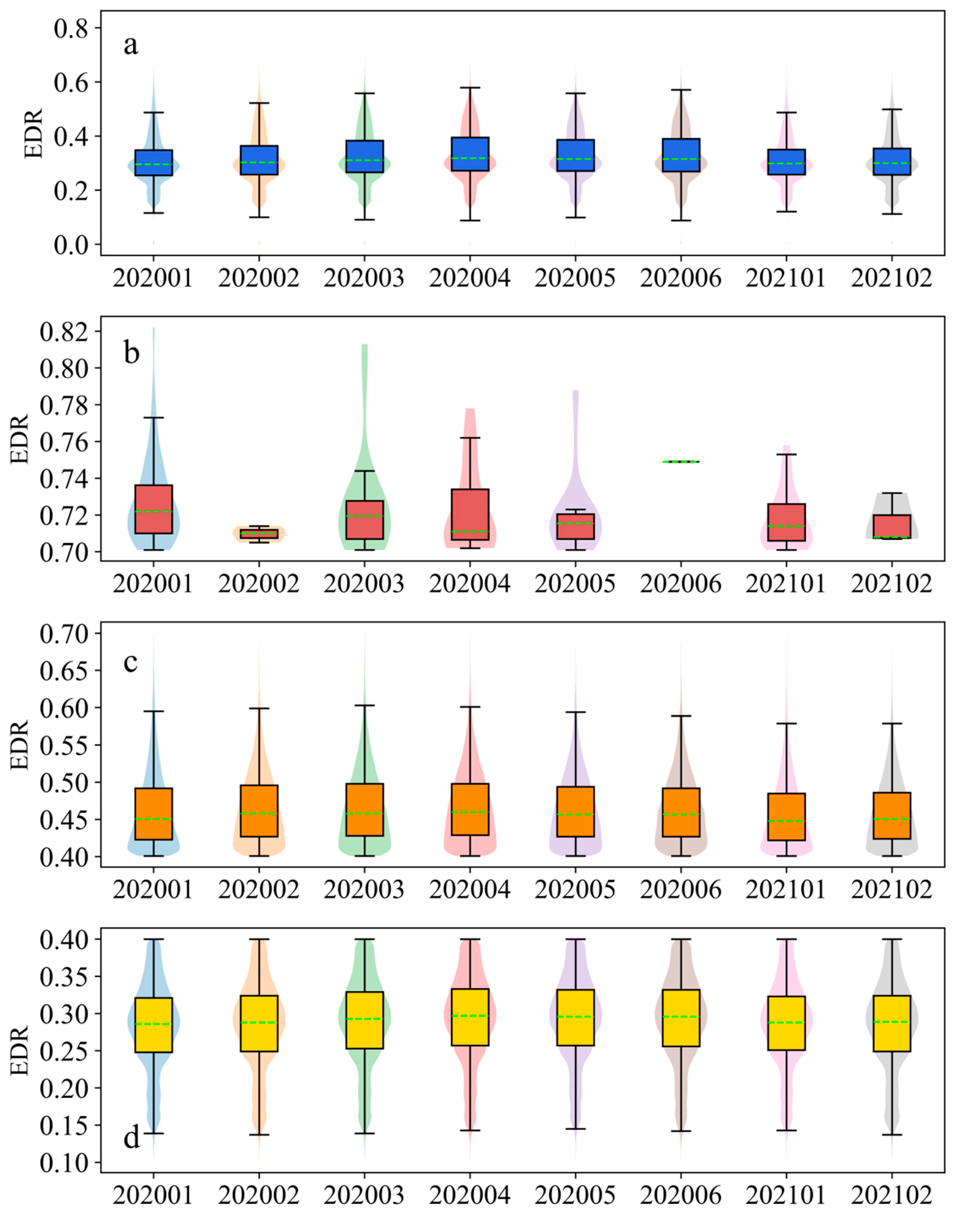
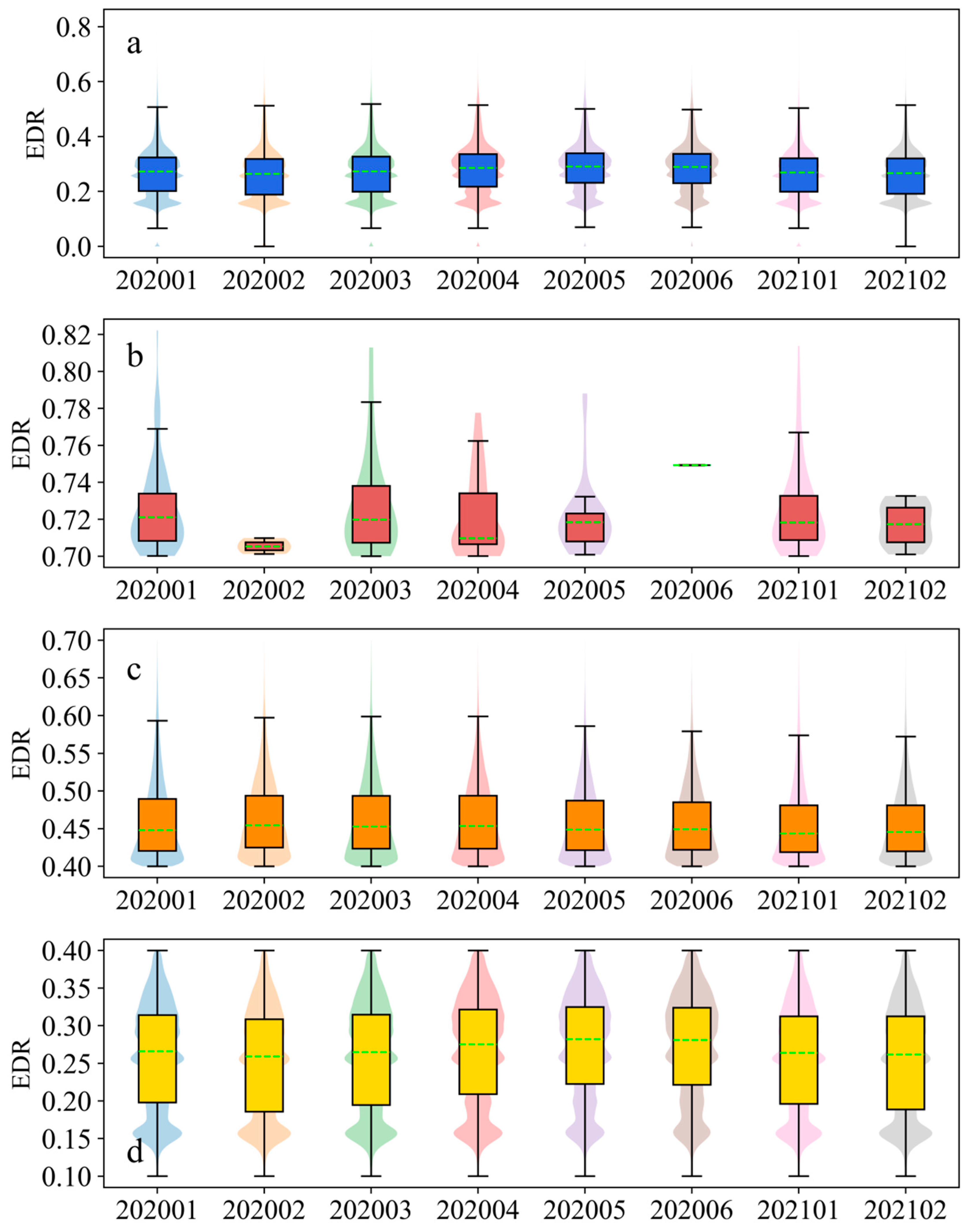
3.1. Monthly Characteristics of Different Aircraft Bumpiness Levels
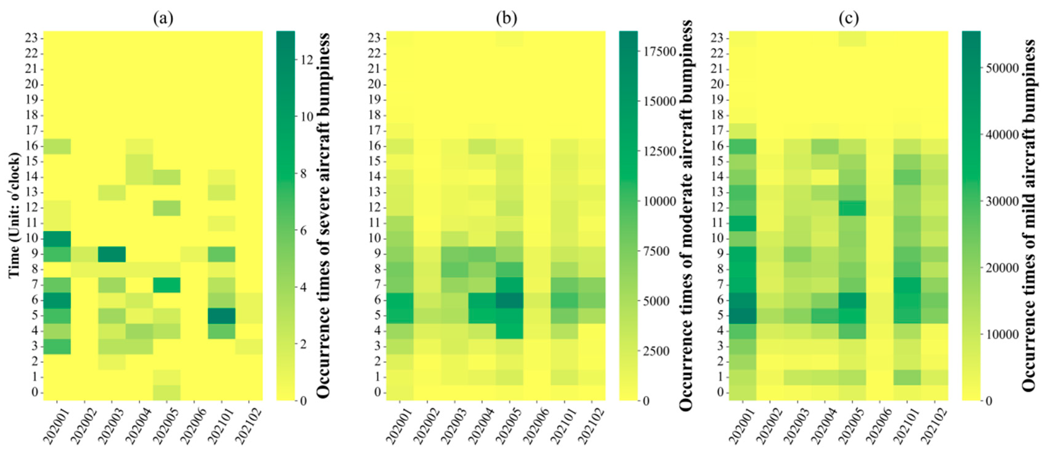
3.2. Intra-Day Characteristics of Different Aircraft Bumpiness Levels
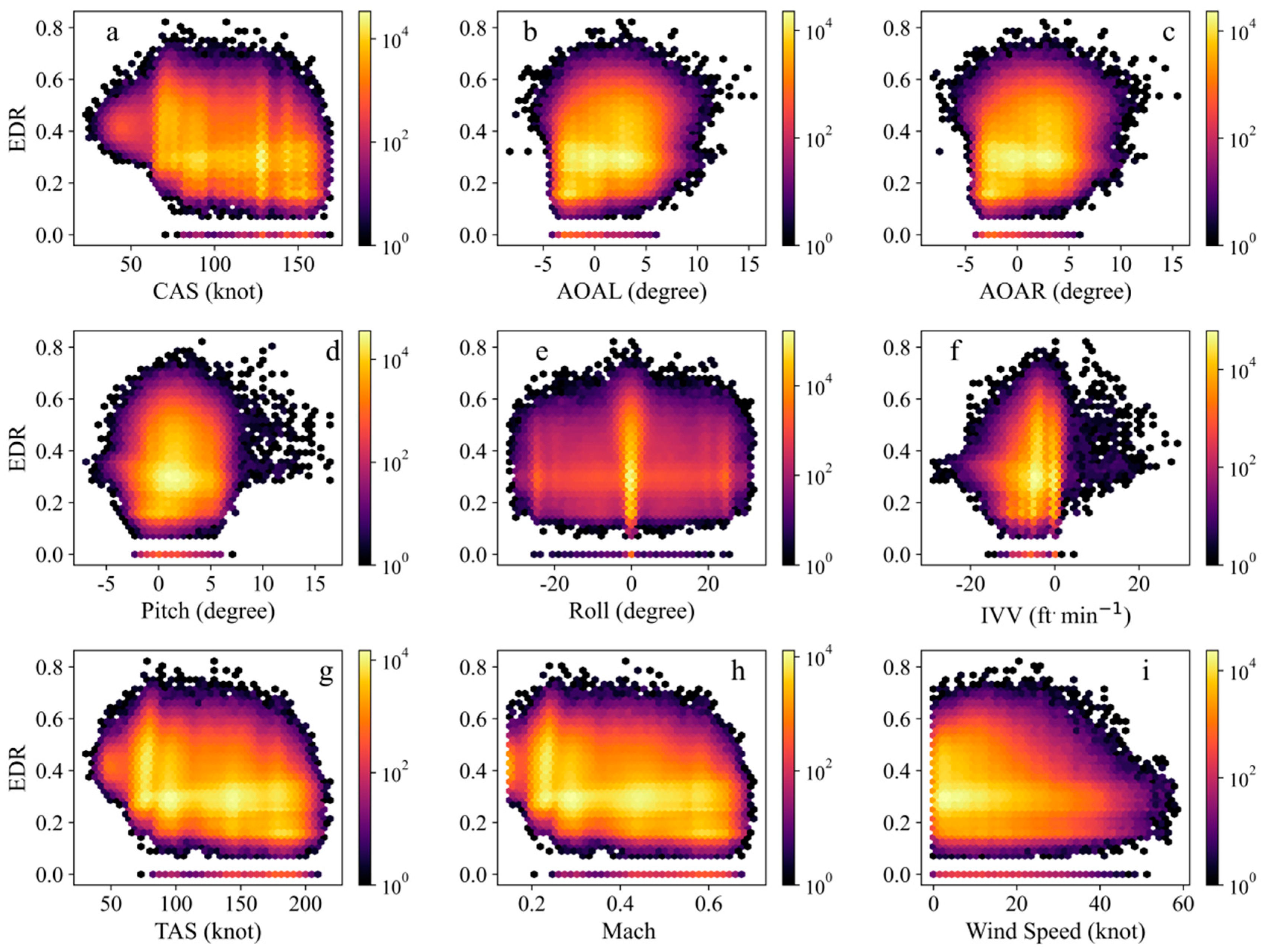
3.3. The Aircraft Flight State when Bumpiness Occurs
3.4. Model Training and Validation
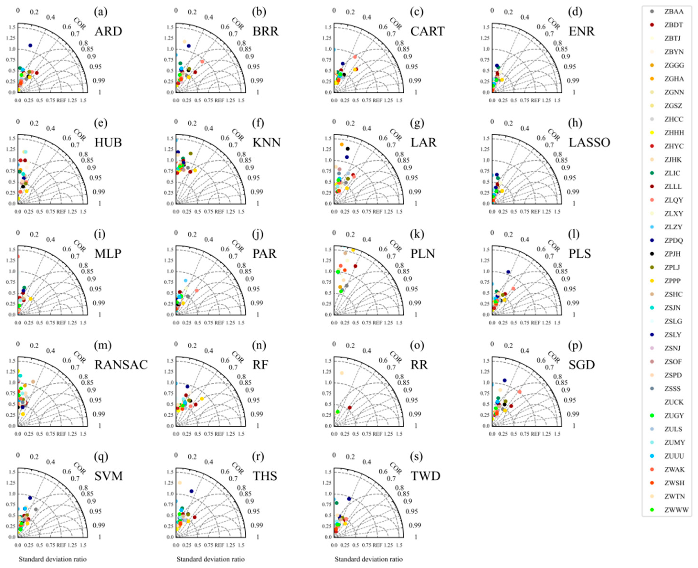
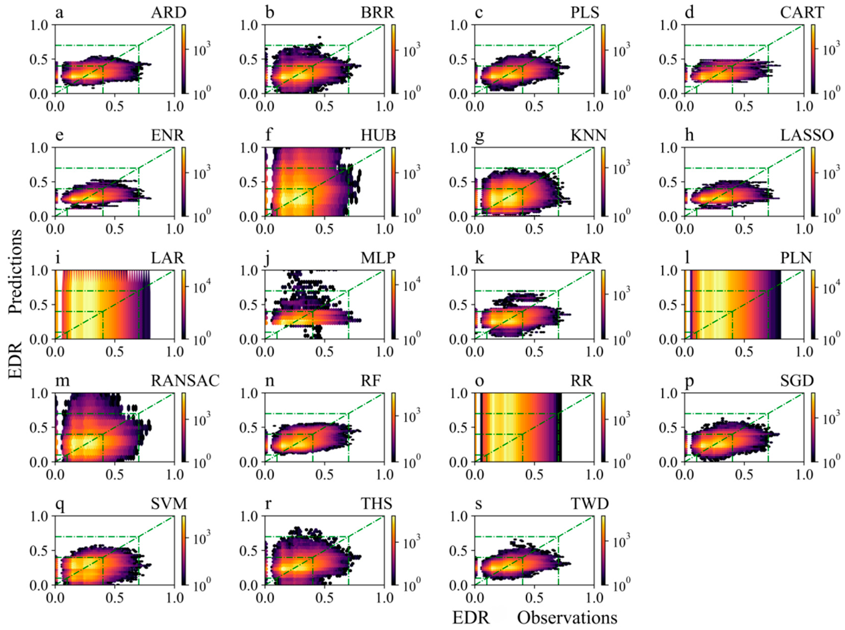
3.4.1. Aircraft Bumpiness Prediction Model for the Airport Approach Areas
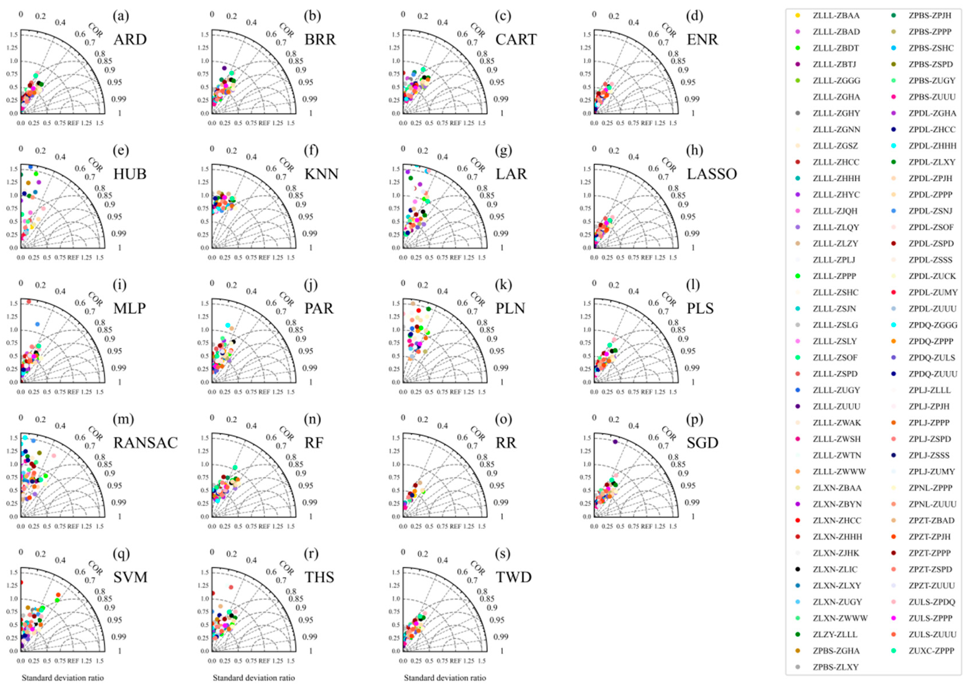
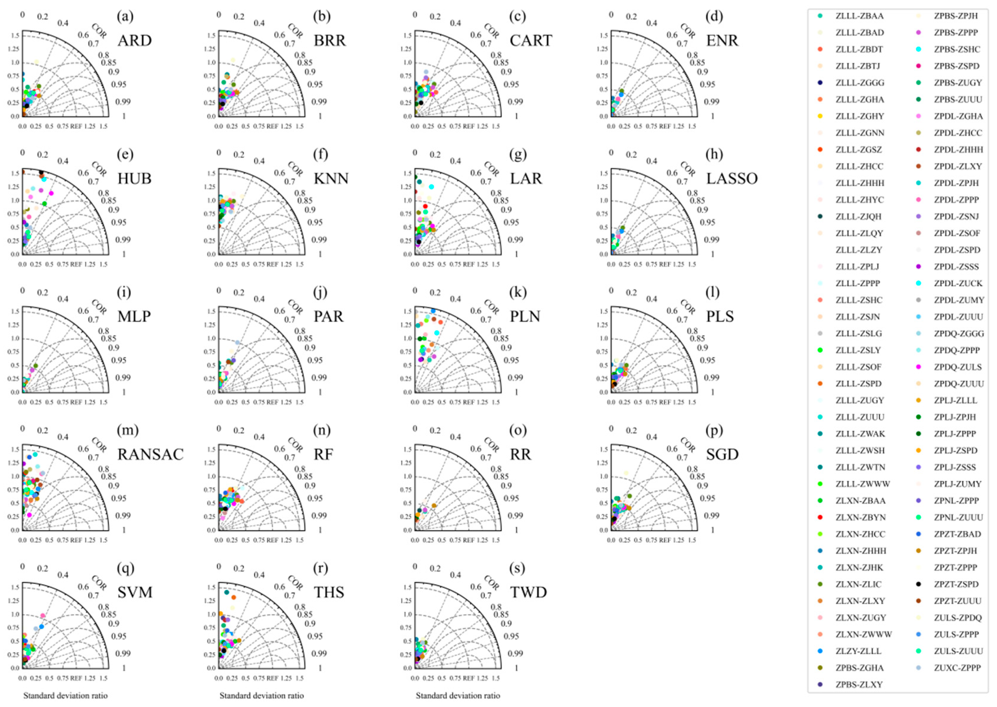
3.4.2. Aircraft Bumpiness Prediction Model for the Flight Routes
4. Discussion
5. Conclusions
- i.
- Severe aircraft bumpiness over the airport approach areas occurred less frequently in February and June 2020, especially in June. For mild aircraft bumpiness, the median EDR from April to June 2020 was higher than in the other months.
- ii.
- Aircraft bumpiness was mainly concentrated between 0:00 a.m. and 17:00 p.m. Severe aircraft bumpiness occurred more frequently in the early morning of January, especially between 5:00 a.m. and 6:00 a.m. The moderate bumpiness occurred from 3:00 a.m. to 11:00 a.m., especially in the early morning (4:00 a.m. to 7:00 a.m.) in April and May 2020.
- iii.
- The relationships between the left and right angles of attack and aircraft bumpiness on the route were more symmetrical with a center at 0 degrees, unlike in the approach areas where the hotspots were mainly concentrated in the range of −5 to 0 degrees. Unlike in the approach areas, the larger the Mach, the more severe the bumpiness was. On the routes, when the Mach number was slightly greater than 0.2, moderate aircraft bumpiness occurred more frequently.
- iv.
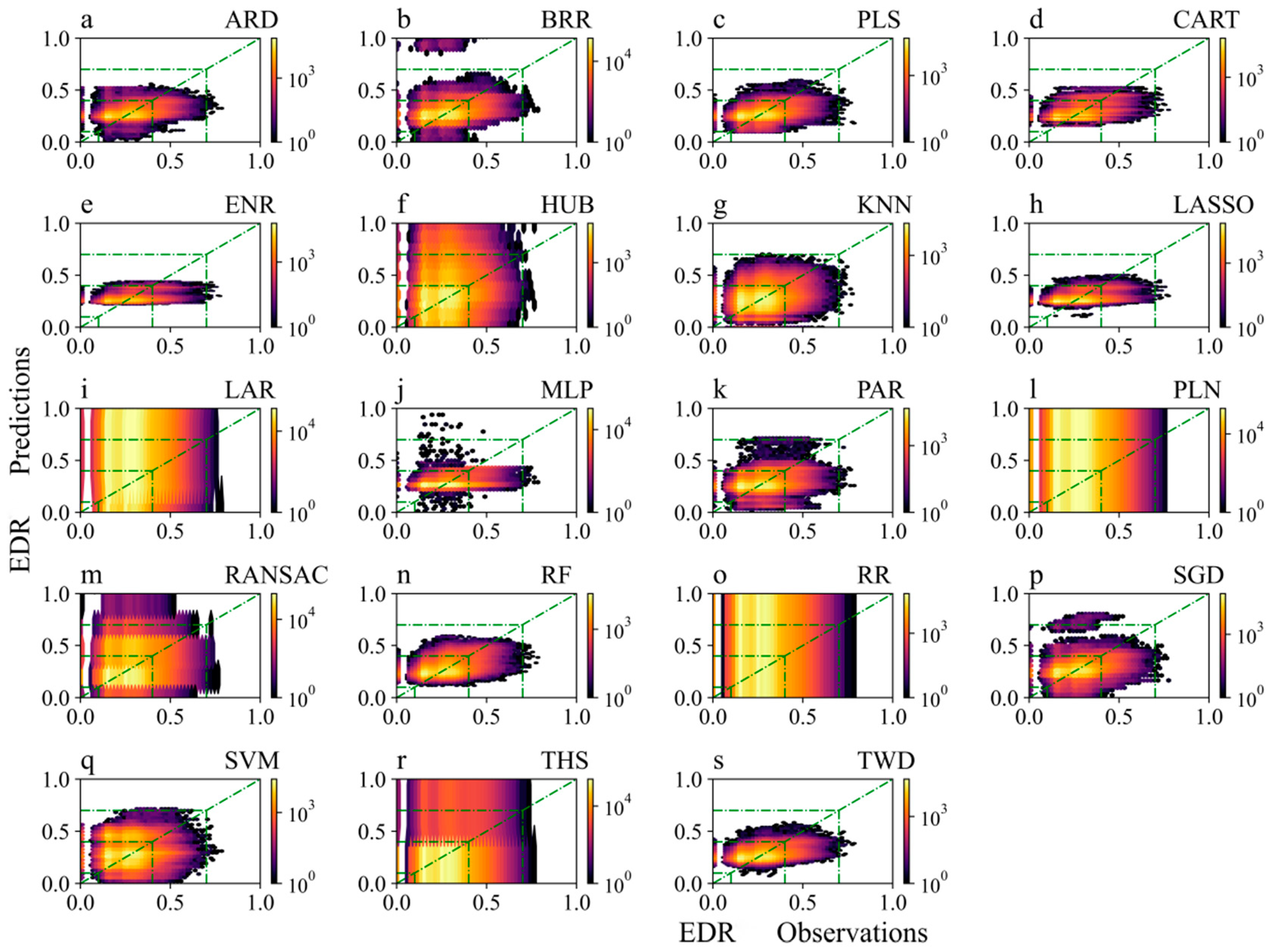
- The performances of the ARD-, PLS-, ENR-, CART-, PAR-, RF-, SGD-, and TWD-based models were relatively good, while the performances of the HUB-, LAR-, PLN-, and RR-based models were very poor. The aircraft bumpiness prediction models performed best over the approach areas of ZBDT in Datong, ZULS in Lhasa, ZPPP in Kunming, and ZLQY in Qingyang. As the prediction time increased, the prediction effect for ZULS decreased the most severely. The aircraft bumpiness prediction model on flight routes for the next 5 min performed best for the ZLLL-ZLQY (Lanzhou–Qingyang), ZPNL-ZPPP (Ninglang–Kunming), and ZLLL-ZBDT (Lanzhou–Datong) routes. As the forecast time increased, in addition to ZLLL-ZBDT, the prediction model for the next 30 min also performed better for the ZPZT-ZPJH (Zhaotong–Xishuangbanna) and ZPDQ-ZULS (Diqing–Lhasa) routes.
Supplementary Materials
Author Contributions
Funding
Institutional Review Board Statement
Informed Consent Statement
Data Availability Statement
Acknowledgments
Conflicts of Interest
References
- Bradshaw, P. An Introduction to Turbulence and Its Measurement; Pergamon Press: Oxford, UK, 1971. [Google Scholar]
- Launder, B.E.; Spalding, D.B. Mathematical Models of Turbulence; Von Karman Institute for Fluid Dynamics: Sint-Genesius-Rode, Belgium, 1972. [Google Scholar]
- Argyropoulos, C.D.; Markatos, N.C. Recent advances on the numerical modelling of turbulent flows. Appl. Math. Model. 2015, 39, 693–732. [Google Scholar] [CrossRef]
- Huang, R.; Sun, H.; Wu, C.; Wang, C.; Lu, B. Estimating Eddy Dissipation Rate with QAR Flight Big Data. Appl. Sci. 2019, 9, 5192. [Google Scholar] [CrossRef]
- Gao, Z.; Wang, H.; Qi, K.; Xiang, Z.; Wang, D. Acceleration-Based In Situ Eddy Dissipation Rate Estimation with Flight Data. Atmosphere 2020, 11, 1247. [Google Scholar] [CrossRef]
- Yanovsky, F.; Prokopenko, I.; Prokopenko, K.; Russchenberg, H.; Ligthart, L. Radar estimation of turbulence eddy dissipation rate in rain. In Proceedings of the IEEE International Geoscience and Remote Sensing Symposium—IGARSS 2002, Toronto, ON, Canada, 24–28 June 2002. [Google Scholar]
- Chan, P.W. LIDAR-based turbulence intensity calculation using glide-path scans of the Doppler LIght Detection and Ranging (LIDAR) systems at the Hong Kong International Airport and comparison with flight data and a turbulence alerting system. Meteorol. Z. 2010, 19, 549–563. [Google Scholar] [CrossRef]
- Hon, K.K.; Chan, P.W. Application of LIDAR-derived eddy dissipation rate profiles in low-level wind shear and turbulence alerts at Hong Kong International Airport. Meteorol. Appl. 2014, 21, 74–85. [Google Scholar] [CrossRef]
- Borque, P.; Luke, E.; Kollias, P. On the unified estimation of turbulence eddy dissipation rate using Doppler cloud radars and lidars. J. Geophys. Res. Atmos. 2016, 121, 5972–5989. [Google Scholar] [CrossRef]
- Yang, S.; Petersen, G.N.; Von Löwis, S.; Preißler, J.; Finger, D.C. Determination of eddy dissipation rate by Doppler lidar in Reykjavik, Iceland. Meteorol. Appl. 2020, 27, e1951. [Google Scholar] [CrossRef]
- Kim, J.-H.; Park, J.-R.; Kim, S.-H.; Kim, J.; Lee, E.; Baek, S.; Lee, G. A Detection of Convectively Induced Turbulence Using in Situ Aircraft and Radar Spectral Width Data. Remote Sens. 2021, 13, 726. [Google Scholar] [CrossRef]
- Emara, M.; Santos, M.D.; Chartier, N.; Ackley, J.; Mavris, D.N. Machine learning enabled turbulence prediction using flight data for safety analysis. In Proceedings of the 32nd Congress of the International Council of the Aeronautical Sciences, Shanghai, China, 6–10 September 2021. [Google Scholar]
- Cai, X.; Wan, Z.; Wu, W.; Yang, B.; Yi, Z. An Ensemble Prediction Method of Aviation Turbulence Based on the Energy Dissipation Rate. Chin. J. Atmos. Sci. 2022, 47, 1085–1098. [Google Scholar] [CrossRef]
- Sharman, R.D.; Pearson, J.M. Prediction of Energy Dissipation Rates for Aviation Turbulence. Part I: Forecasting Nonconvective Turbulence. J. Appl. Meteorol. Clim. 2017, 56, 317–337. [Google Scholar] [CrossRef]
- Pearson, J.M.; Sharman, R.D. Prediction of Energy Dissipation Rates for Aviation Turbulence. Part II: Nowcasting Convective and Nonconvective Turbulence. J. Appl. Meteorol. Clim. 2017, 56, 339–351. [Google Scholar] [CrossRef]
- Muñoz-Esparza, D.; Sharman, R.; Sauer, J.; Kosović, B. Toward Low-Level Turbulence Forecasting at Eddy-Resolving Scales. Geophys. Res. Lett. 2018, 45, 8655–8664. [Google Scholar] [CrossRef]
- Kim, J.-H.; Sharman, R.; Strahan, M.; Scheck, J.W.; Bartholomew, C.; Cheung, J.C.H.; Buchanan, P.; Gait, N. Improvements in Nonconvective Aviation Turbulence Prediction for the World Area Forecast System. Bull. Am. Meteorol. Soc. 2018, 99, 2295–2311. [Google Scholar] [CrossRef]
- Lee, D.-B.; Chun, H.-Y.; Kim, S.-H.; Sharman, R.D.; Kim, J.-H. Development and Evaluation of Global Korean Aviation Turbulence Forecast Systems Based on an Operational Numerical Weather Prediction Model and In Situ Flight Turbulence Observation Data. Weather Forecast 2022, 37, 371–392. [Google Scholar] [CrossRef]
- Chen, H.; Pang, L.; Wanyan, X.; Liu, S.; Fang, Y.; Tao, D. Effects of Air Route Alternation and Display Design on an Operator’s Situation Awareness, Task Performance and Mental Workload in Simulated Flight Tasks. Appl. Sci. 2021, 11, 5745. [Google Scholar] [CrossRef]
- Shu, Y.; Zhu, Y.; Xu, F.; Gan, L.; Lee, P.T.-W.; Yin, J.; Chen, J. Path planning for ships assisted by the icebreaker in ice-covered waters in the Northern Sea Route based on optimal control. Ocean Eng. 2023, 267, 113182. [Google Scholar] [CrossRef]
- Chen, X.; Wang, Z.; Hua, Q.; Shang, W.-L.; Luo, Q.; Yu, K. AI-Empowered Speed Extraction via Port-Like Videos for Vehicular Trajectory Analysis. IEEE Trans. Intell. Transp. Syst. 2022, 24, 4541–4552. [Google Scholar] [CrossRef]
- Williams, J.K. Using random forests to diagnose aviation turbulence. Mach. Learn. 2014, 95, 51–70. [Google Scholar] [CrossRef]
- Muñoz-Esparza, D.; Sharman, R.D.; Deierling, W. Aviation Turbulence Forecasting at Upper Levels with Machine Learning Techniques Based on Regression Trees. J. Appl. Meteorol. Clim. 2020, 59, 1883–1899. [Google Scholar] [CrossRef]
- Sridhar, B. Applications of Machine Learning Techniques to Aviation Operations: Promises and Challenges. In Proceedings of the 2020 International Conference on Artificial Intelligence and Data Analytics for Air Transportation (AIDA-AT), Singapore, 3–4 February 2020; pp. 1–12. [Google Scholar] [CrossRef]
- Cordeiro, F.M.; França, G.B.; Neto, F.L.d.A.; Gultepe, I. Visibility and Ceiling Nowcasting Using Artificial Intelligence Techniques for Aviation Applications. Atmosphere 2021, 12, 1657. [Google Scholar] [CrossRef]
- Ding, J.; Zhang, G.; Wang, S.; Xue, B.; Yang, J.; Gao, J.; Wang, K.; Jiang, R.; Zhu, X. Forecast of Hourly Airport Visibility Based on Artificial Intelligence Methods. Atmosphere 2022, 13, 75. [Google Scholar] [CrossRef]
- Ding, J.; Zhang, G.; Yang, J.; Wang, S.; Xue, B.; Du, X.; Tian, Y.; Wang, K.; Jiang, R.; Gao, J. Temporal and Spatial Characteristics of Meteorological Elements in the Vertical Direction at Airports and Hourly Airport Visibility Prediction by Artificial Intelligence Methods. Sustainability 2022, 14, 12213. [Google Scholar] [CrossRef]
- Mizuno, S.; Ohba, H.; Ito, K. Machine learning-based turbulence-risk prediction method for the safe operation of aircrafts. J. Big Data 2022, 9, 29. [Google Scholar] [CrossRef]
- Wang, L.; Wu, C.; Sun, R. An analysis of flight Quick Access Recorder (QAR) data and its applications in preventing landing incidents. Reliab. Eng. Syst. Saf. 2014, 127, 86–96. [Google Scholar] [CrossRef]
- Abernethy, J.A.; Sharman, R.; Bradley, E. Application of artificial intelligence to operational real-time clear-air turbulence prediction. In Proceedings of the Twenty-Third AAAI Conference on Artificial Intelligence—AAAI 2008, Chicago, IL, USA, 13–17 July 2008. [Google Scholar]
- Oliveira, M.M.; Mayor, G.S.; Macedo, J.P.; Bidinotto, J.H. Neural networks to classify atmospheric turbulence from flight test data: An optimization of input parameters for a generic model. J. Braz. Soc. Mech. Sci. Eng. 2022, 44, 82. [Google Scholar] [CrossRef]
- Breiman, L. Random forests. Mach. Learn. 2001, 45, 5–32. [Google Scholar] [CrossRef]
- Cristianini, N.; Taylor, J.S. An Introduction to Support Vector Machines and Other Kernel-Based Learning Methods; University Press: Cambridge, UK, 2000. [Google Scholar]
- Avila, J.; Hauck, T. Least angle regression. Ann. Stat. 2004, 32, 407–499. [Google Scholar] [CrossRef]
- Robbins, H.; Monro, S. A Stochastic Approximation Method. Ann. Math. Stat. 1951, 22, 400–407. [Google Scholar] [CrossRef]
- MacKay, D.J.C. Bayesian Interpolation. Neural Comput. 1992, 4, 415–447. [Google Scholar] [CrossRef]
- Tipping, M.E. Sparse bayesian learning and the relevance vector machine. J. Mach. Learn. Res. 2001, 1, 211–244. [Google Scholar] [CrossRef]
- Tibshirani, R. Regression shrinkage and selection via the lasso. J. R. Stat. Soc. Ser. B Methodol. 1996, 58, 267–288. [Google Scholar] [CrossRef]
- Crammer, K.; Dekel, O.; Keshet, J.; Shalev-Shwartz, S.; Singer, Y.; Warmuth, M.K. Online passive-aggressive algorithms. J. Mach. Learn. Res. 2006, 7, 551–585. [Google Scholar] [CrossRef]
- Fischler, M.A.; Bolles, R.C. Random sample consensus: A paradigm for model fitting with applications to image analysis and automated cartography. Commun. ACM 1981, 24, 619–638. [Google Scholar] [CrossRef]
- Huber, P.J. A Robust Version of the Probability Ratio Test. Ann. Math. Stat. 1965, 36, 1753–1758. [Google Scholar] [CrossRef]
- Huber, P.J. Robust Regression: Asymptotics, Conjectures and Monte Carlo. Ann. Stat. 1973, 1, 799–881. [Google Scholar] [CrossRef]
- Durbin, R.; Willshaw, D. An analogue approach to the travelling salesman problem using an elastic net method. Nature 1987, 326, 689–691. [Google Scholar] [CrossRef]
- Mackay, D.J.C. Bayesian Non-Linear Modeling for the Energy Prediction Competition. In Proceedings of the 1994 American Society of Heating, Refrigerating, and Air Conditioning Engineers (ASHRAE), Orlando, FL, USA, 25–29 June 1994; Volume 100. [Google Scholar]
- Thiel, H. A Rank-Invariant Method of Linear and Polynomial Regression Analysis. Proc. Proc. Kon. Ned. Akad. Wet. Ser. A Math. Sci. 1950, 53, 386–392. [Google Scholar]
- Sen, P.K. Estimates of the regression coefficient based on Kendall’s Tau. J. Am. Stat. Assoc. 1968, 63, 1379–1389. [Google Scholar] [CrossRef]
- Jin, C.; Guo, W.; Gan, L.; Wang, C. Statistics and possible sources of low-level turbulence below 3000 m and its meteorological condition in beijing. J. Meteorol. Environ. 2019, 35, 18–26. [Google Scholar]
- Fang, L. Research on the Characteristics and Causes of High Altitude Aircraft Bump Based on Aircraft Detection Data; Civil Aviation Flight University of China: Deyang, China, 2022. [Google Scholar] [CrossRef]
- Wang, S. Research on the Influence of Terrain on Aircraft Bumping; Civil Aviation Flight University of China: Deyang, China, 2022. [Google Scholar] [CrossRef]
- Xu, J.; Wang, D.; Gong, Y.; Duan, Y. Quantitative diagnostic and distribution characteristics of aircraft turbulence in China. J. Chengdu Univ. Inf. Technol. 2018, 33, 704–712. [Google Scholar] [CrossRef]
- Li, C. Research on the Main Temporal and Spatial Distribution Characteristics of Aircraft Turbulence in China; Civil Aviation Flight University of China: Deyang, China, 2018. (In Chinese) [Google Scholar]


| No. | Abbreviation | Unit | Interpretation |
|---|---|---|---|
| 1 | G | g | Vertical acceleration |
| 2 | Alt | foot | Altitude |
| 3 | CAS | knot | Calibrated airspeed |
| 4 | AOAL | degree | Angle of attack (left) |
| 5 | AOAR | degree | Angle of attack (right) |
| 6 | Pitch | degree | Pitching angle |
| 7 | Pitch rate | degree/s | |
| 8 | Roll | degree | Roll angle |
| 9 | IVV | feet/minute | Instantaneous lifting velocity |
| 10 | TAS | knot | True airspeed |
| 11 | Mach | Mach number | |
| 12 | Lat | degree | Latitude |
| 13 | Lon | degree | Longitude |
| 14 | windSpd | knot | Wind speed |
| 15 | windDir | degree | Computed wind direction |
| 16 | Date |
| Flight Route | Departure and Arrival Locations | Flight Route | Departure and Arrival Locations | ||
|---|---|---|---|---|---|
| 1 | ZLLL-ZBAA | Lanzhou/Beijing | 42 | ZPBS-ZPJH | Longyang/Xishuangbanna |
| 2 | ZLLL-ZBAD | Lanzhou/Beijing | 43 | ZPBS-ZPPP | Longyang/Kunming |
| 3 | ZLLL-ZBDT | Lanzhou/Datong | 44 | ZPBS-ZSHC | Longyang/Hangzhou |
| 4 | ZLLL-ZBTJ | Lanzhou/Tianjin | 45 | ZPBS-ZSPD | Longyang/Shanghai |
| 5 | ZLLL-ZGGG | Lanzhou/Guangzhou | 46 | ZPBS-ZUGY | Longyang/Guiyang |
| 6 | ZLLL-ZGHA | Lanzhou/Changsha | 47 | ZPBS-ZUUU | Longyang/Chengdu |
| 7 | ZLLL-ZGHY | Lanzhou/Hengyang | 48 | ZPDL-ZGHA | Dali/Changsha |
| 8 | ZLLL-ZGNN | Lanzhou/Nanning | 49 | ZPDL-ZHCC | Dali/Zhengzhou |
| 9 | ZLLL-ZGSZ | Lanzhou/Shenzhen | 50 | ZPDL-ZHHH | Dali/Wuhan |
| 10 | ZLLL-ZHCC | Lanzhou/Zhengzhou | 51 | ZPDL-ZLXY | Dali/Xian |
| 11 | ZLLL-ZHHH | Lanzhou/Wuhan | 52 | ZPDL-ZPJH | Dali/Xishuangbanna |
| 12 | ZLLL-ZHYC | Lanzhou/Yichang | 53 | ZPDL-ZPPP | Dali/Kunming |
| 13 | ZLLL-ZJQH | Lanzhou/Qionghai | 54 | ZPDL-ZSNJ | Dali/Nanjing |
| 14 | ZLLL-ZLQY | Lanzhou/Qingyang | 55 | ZPDL-ZSOF | Dali/Hefei |
| 15 | ZLLL-ZLZY | Lanzhou/Zhangye | 56 | ZPDL-ZSPD | Dali/Shanghai |
| 16 | ZLLL-ZPLJ | Lanzhou/Lijiang | 57 | ZPDL-ZSSS | Dali/Shanghai |
| 17 | ZLLL-ZPPP | Lanzhou/Kunming | 58 | ZPDL-ZUCK | Dali/Chongqing |
| 18 | ZLLL-ZSHC | Lanzhou/Hangzhou | 59 | ZPDL-ZUMY | Dali/Mianyang |
| 19 | ZLLL-ZSJN | Lanzhou/Jinan | 60 | ZPDL-ZUUU | Dali/Chengdu |
| 20 | ZLLL-ZSLG | Lanzhou/Lianyungang | 61 | ZPDQ-ZGGG | Diqing/Guangzhou |
| 21 | ZLLL-ZSLY | Lanzhou/Linyi | 62 | ZPDQ-ZPPP | Diqing/Kunming |
| 22 | ZLLL-ZSOF | Lanzhou/Hefei | 63 | ZPDQ-ZULS | Diqing/Lhasa |
| 23 | ZLLL-ZSPD | Lanzhou/Shanghai | 64 | ZPDQ-ZUUU | Diqing/Chengdu |
| 24 | ZLLL-ZUGY | Lanzhou/Guiyang | 65 | ZPLJ-ZLLL | Lijiang/Lanzhou |
| 25 | ZLLL-ZUUU | Lanzhou/Chengdu | 66 | ZPLJ-ZPJH | Lijiang/Xishuangbanna |
| 26 | ZLLL-ZWAK | Lanzhou/Akesu | 67 | ZPLJ-ZPPP | Lijiang/Kunming |
| 27 | ZLLL-ZWSH | Lanzhou/Kashi | 68 | ZPLJ-ZSPD | Lijiang/Shanghai |
| 28 | ZLLL-ZWTN | Lanzhou/Hetian | 69 | ZPLJ-ZSSS | Lijiang/Shanghai |
| 29 | ZLLL-ZWWW | Lanzhou/Urumqi | 70 | ZPLJ-ZUMY | Lijiang/Mianyang |
| 30 | ZLXN-ZBAA | Xining/Beijing | 71 | ZPNL-ZPPP | Ninglang/Kunming |
| 31 | ZLXN-ZBYN | Xining/Taiyuan | 72 | ZPNL-ZUUU | Ninglang/Chengdu |
| 32 | ZLXN-ZHCC | Xining/Zhengzhou | 73 | ZPZT-ZBAD | Zhaotong/Beijing |
| 33 | ZLXN-ZHHH | Xining/Wuhan | 74 | ZPZT-ZPJH | Zhaotong/Xishuangbanna |
| 34 | ZLXN-ZJHK | Xining/Zhuhai | 75 | ZPZT-ZPPP | Zhaotong/Kunming |
| 35 | ZLXN-ZLIC | Xining/Yinchuan | 76 | ZPZT-ZSPD | Zhaotong/Shanghai |
| 36 | ZLXN-ZLXY | Xining/Xian | 77 | ZPZT-ZUUU | Zhaotong/Chengdu |
| 37 | ZLXN-ZUGY | Xining/Guiyang | 78 | ZULS-ZPDQ | Lhasa/Diqing |
| 38 | ZLXN-ZWWW | Xining/Urumqi | 79 | ZULS-ZPPP | Lhasa/Kunming |
| 39 | ZLZY-ZLLL | Zhangye/Lanzhou | 80 | ZULS-ZUUU | Lhasa/Chengdu |
| 40 | ZPBS-ZGHA | Longyang/Changsha | 81 | ZUXC-ZPPP | Xichang/Kunming |
| 41 | ZPBS-ZLXY | Longyang/Xian |
Disclaimer/Publisher’s Note: The statements, opinions and data contained in all publications are solely those of the individual author(s) and contributor(s) and not of MDPI and/or the editor(s). MDPI and/or the editor(s) disclaim responsibility for any injury to people or property resulting from any ideas, methods, instructions or products referred to in the content. |
© 2023 by the authors. Licensee MDPI, Basel, Switzerland. This article is an open access article distributed under the terms and conditions of the Creative Commons Attribution (CC BY) license (https://creativecommons.org/licenses/by/4.0/).
Share and Cite
Ding, J.; Zhang, G.; Wang, S.; Xue, B.; Wang, K.; Yu, T.; Jiang, R.; Chen, Y.; Huang, Y.; Li, Z.; et al. Characteristic Analysis and Short-Impending Prediction of Aircraft Bumpiness over Airport Approach Areas and Flight Routes. Atmosphere 2023, 14, 1704. https://doi.org/10.3390/atmos14111704
Ding J, Zhang G, Wang S, Xue B, Wang K, Yu T, Jiang R, Chen Y, Huang Y, Li Z, et al. Characteristic Analysis and Short-Impending Prediction of Aircraft Bumpiness over Airport Approach Areas and Flight Routes. Atmosphere. 2023; 14(11):1704. https://doi.org/10.3390/atmos14111704
Chicago/Turabian StyleDing, Jin, Guoping Zhang, Shudong Wang, Bing Xue, Kuoyin Wang, Tingzhao Yu, Ruijiao Jiang, Yu Chen, Yan Huang, Zhimin Li, and et al. 2023. "Characteristic Analysis and Short-Impending Prediction of Aircraft Bumpiness over Airport Approach Areas and Flight Routes" Atmosphere 14, no. 11: 1704. https://doi.org/10.3390/atmos14111704