Article

Experimental Study of Particle Transport and Deposition Distribution over Complex Terrains Based on Spherical Alumina

1
Key Laboratory of Mechanics on Disaster and Environment in Western China, Lanzhou University, Lanzhou 730000, China
2
College of Civil Engineering and Mechanics, Lanzhou University, Lanzhou 730000, China
3
School of Information Engineering, Lanzhou City University, Lanzhou 730070, China
*
Authors to whom correspondence should be addressed.
Atmosphere 2023, 14(12), 1756; https://doi.org/10.3390/atmos14121756
Submission received: 7 October 2023 / Revised: 26 November 2023 / Accepted: 27 November 2023 / Published: 29 November 2023

Abstract

:
The transport and deposition of atmospheric particulate matter have attracted significant attention recently due to the increasing frequency of extreme disaster events, such as dust storms, volcanic eruptions, and extensive forest fires. The size distribution of the transported material and the conditions of the land–air interface are dominant factors in comprehending the detrimental potential of atmospheric particulate matter. However, it is still a challenge to understand the mechanism of dust deposition, especially over complex terrain. In an effort to investigate the deposition characteristics of particles over complex terrain, a series of experiments were conducted in a multifunctional environmental wind tunnel. The results show that the wind speed directly above the top of the mild slope model is significantly greater than that in the steep slope model, which indicates that a steep slope has a greater blocking effect on wind fields. At low wind speeds, the average wind speed at the top of the mild slope model is 17.8% higher than that at the top of the steep slope model, and at high wind speeds the average wind speed at the top of the mild slope model is 8.6% higher than that at the top of the steep slope model. The influence trend of the steep slope model and the combination model is basically the same, with both decreasing first and then increasing with the direction of wind velocity. The amount of surface deposition is greatly affected by the location of the feeding point and the microscale characteristics of the surface. In the steep slope model, the deposition is mainly distributed on the windward side, while the leeward side has a small amount of deposition. In the mild slope model, particles are deposited not only on the windward side, but also on the leeward side. The average rate of decline in deposition flux in the steep slope model is 88.4% and 75.1% in the mild slope model. The use of the combination model reduces the particle concentration at the back end compared with the single model. In three different models, the deposition on the windward side was shown to be significantly greater than that on the leeward side of the model. Our work increases understanding of the deposition of coarse dust particles over complex terrain and provides basic data for improving the accuracy of large-region particle transport and deposition simulations.

1. Introduction

The transport and deposition processes of dust particles occur widely in nature, and have complex interactions with many major systems and processes, such as the physical climate system [1], the biogeochemical cycle [2,3], geomorphic evolution [4], the water cycle [5], and the ecosystem [6,7]. Specific manifestations include near-surface sandstorm transport [8,9], large-scale sandstorms [10], and volcanic eruptions [11,12], which cause threats to buildings [13], transportation [14], water resources [15], communication equipment [16], agriculture [17], and human health [18,19]. Therefore, clarifying the transport and deposition laws of dust particles is of practical significance for the simulation [20], prediction [21], risk assessment, and disaster prevention of global wind erosion processes and the dust cycle.
Although meteorological models or software can gather and process meteorological data effectively to improve the accuracy of simulations of dust transport, most calculations for large-scale dust particle transport processes are carried out by solving scalar matter conservation equations coupled with fluid equations [22,23]. In the calculation process, it is assumed that scalar matter follows the same movement pattern as fluids (in fact, only small-sized particles can satisfy this assumption), which is inconsistent with reality, as sand contains particles of multiple sizes [24,25]. Although there are numerous calculation models that can simulate the dispersal of sand and dust in the atmospheric transport stage and provide a prediction of ground deposition, the behavior of particles of different sizes in atmospheric transport is generally distinguished only by different deposition velocities [26]. When calculating the horizontal wind movement of particles with different sizes, the complete wind movement calculation model is mostly adopted, and the same turbulent diffusion parameters are used to describe the diffusion behavior of sand with different particle sizes, without considering the complex interaction between particles and turbulence or even reflecting the difference in the turbulent diffusion effect of particles with different sizes [27,28]. In fact, according to the research results of gas–solid two-phase flow obtained in recent years, the change in velocity of solid particles in a wind field generally lags behind the change in the velocity of the wind field itself, and this degree of hysteresis is closely related to particle size inertia. However, the existing deposition calculation model does not take into account the motion separation effect of the gas–solid phase caused by particle inertia, which becomes a bottleneck in the accurate prediction of dust transport and deposition.
In a wide and flat location, the horizontal and vertical changes in wind and turbulence fields are relatively small, the flow field is close to stable and uniform, and the particle diffusion state mostly follows a normal probability distribution. Therefore, when using a simple Gaussian model [29] to predict the impact of the atmospheric environment, a prediction result that correlates highly with the actual value can be obtained. However, over complex terrain, due to the influence of the terrain, the wind field and turbulence field change dramatically, both spatially and temporally, and the diffusion process is much more complicated than that in flat areas [30]. This makes the prediction of previous models significantly different from the actual state, and causes great difficulties in the accurate prediction of the atmospheric environment under complex terrain [31,32], particularly in the prediction of ash deposition after volcanic eruptions [33,34]. At present, wind tunnel experiments are often used to summarize and analyze the transport and deposition laws of dust particles in the study of complex terrain, so as to improve the deposition scheme on the basis of a large number of experimental data [35]. Zufall et al. [36,37] used wind tunnel experiments to simulate and measure the dry deposition process of particles on a wavy surface. Lin and Khlystov [38] further studied the deposition of ultrafine particles on complex surfaces and found that the deposition efficiency decreased with the increase in particle size, wind speed, and deposition density. Parker and Kinnersley [39] focused on the study of the impact of topographic changes on the deposition of small particles, and found that the amount of deposit on the leeward side was large but the area was small, and the amount of deposit in the wake area was small but the area was large. However, relatively little work has been carried out on large-particle dry deposits that have important environmental impacts on complex terrain.
Kok et al. [40] counted and analyzed a large number of observational data, and found that coarse and super coarse dust particles (D > 10 µm) are transported farther than previously expected, and that the abundance of these particles has been greatly underestimated in current global models. Because these limitations largely lead to uncertainties in modelling the abundance and effects of coarse dust and super coarse dust aerosols, an accurate representation of coarse and super coarse properties is critical to understanding the overall impact of dust aerosols on the Earth’s systems.
Atmospheric deposition is an important process affected by man-made and natural factors, and the lack of deposition flux data over complex terrain such as mountains leads to relatively few studies. In the paper, spherical alumina was used as the experimental particle to simulate the transport and deposition process of heavy particles, whose abundance has been greatly underestimated in previous models. In order to further understand and reveal the dynamic mechanism of the influence of surface obstacles on the spatial distribution of heavy particle settlement, we simulated two wind conditions (5 m·s−1, 10 m·s−1) and four landforms (flat land, steep slope model A, mild slope model B, and combination model AB of a steep slope in front and a mild slope behind) in a wind tunnel. The statistical laws of wind speed, particle velocity, and surface deposition flux were obtained using a hot-wire anemometer, particle image velocity (PIV), and surface deposition measurements. Through the work in this paper, we hope to increase understanding of the deposition mechanism and law of coarse dust particles on complex terrain, and provide basic data for improving the accuracy of simulations and predictions of global wind erosion processes and the dust cycle.

2. Materials and Methods

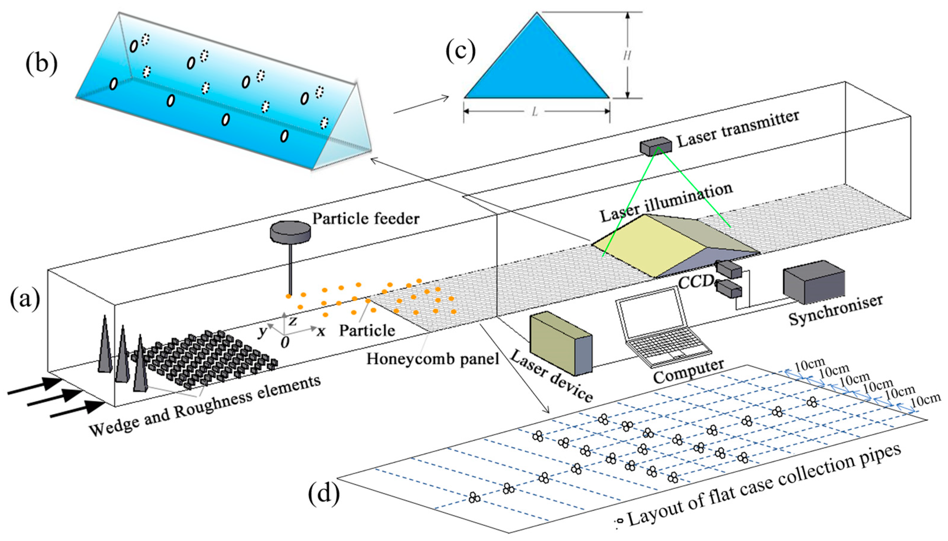
2.1. Wind Tunnel Experimental Environment Settings

The experiment was carried out in the U-shaped boundary layer wind tunnel of Lanzhou University of Technology. The wind tunnel is designed for the simulation of a large gas boundary layer wind environment. Its test section is 12 m long, 2 m wide, and 2 m high. The designed wind speed is adjustable from 1 to 20 m·s−1, and the wind turbulence is less than 1%. In order to realize the logarithmic wind velocity profile in the atmospheric boundary layer, we arranged wedge and rough elements in succession at the entrance of the wind tunnel. Among these elements, the height of the wedge was 0.3 m, the base was 0.1 m, and the spacing between the three wedges was 0.3 m. At 0.64 m downwind of the wedge, a 1.8 m long rough element array was arranged to efficiently reduce the near-surface wind speed. At 0.94 m downwind of the rough element array, a self-made particle feeder was installed on the top of the wind tunnel to simulate the airborne release, transport, and deposition behavior of dust particles. The inner diameter of the release pipe of the feeder was 22 mm, which can be regarded as the case of point-source release. This has been widely used in the construction of dust transport models as a simplified description of volcanic eruption [41,42] and chimney emission [43]. In order to conduct subsequent statistical analysis on the dust transport and deposition process, we took the projection of the feed point perpendicular to the bottom plate of the wind tunnel as the origin of the coordinates, the direction of flow as the positive direction of the x-axis, the spread direction as the positive direction of the y-axis, and the vertical direction as the positive direction of the z-axis, and established the Cartesian right-handed coordinate system. In order to meet the requirements of dust transport distance as much as possible, an interval of 1.5–8.5 m in this coordinate system was set as the experimental observation area, in which the mountain model and PIV observation equipment were placed. It is worth noting that in order to avoid horizontal water transport caused by sand particles falling and hitting the solid surface, we laid honeycomb panels at the bottom of the wind tunnel in the experimental observation area, which were able to effectively capture and simulate the settling behavior of sand particles in a real environment, and were also conducive to the subsequent collection of deposit samples. The overall experimental arrangement is shown in Figure 1.
The Froude number is a dimensionless parameter that expresses the relative magnitude of the inertia force and gravity of a fluid. Here, the Froude number (Fr) is expressed as follows:
F r = U 2 g H t ,
where U is the incoming wind velocity (2.5–13.0 m·s−1); the gravitational acceleration g is 9.8 m·s−2. Ht means the height of the wind tunnel is 2 m. According to the literature [44], the disturbance of the flow direction pressure gradient is avoided by satisfying the Froude number, that is, Fr < 20 is required in the wind tunnel experiment. The maximum Fr in this paper is 8.6, which meets the experimental requirements.
To analyze the effect of the model on particle deposition, we introduced the obstacle Reynolds number (Reo) [45], which is expressed as follows:
R e o = U L A μ ,
L A = L 1 3 H 2 3 ,
where the dynamic viscosity of the atmosphere μ is 1.8 × 10⁻⁵ Pa·s. LA is the equivalent length of the frontal obstacle area involving obstacle height H and width L. Reo, hence, indicates the erosive potential and turbulent energy of the downwind obstacle.

2.2. Observation Equipment and Particle Samples

In this paper, particle image velocity (PIV) measurement was used to observe the complex particle velocity and concentration distribution around the mountain model. PIV is advantageous as it can be carried out quickly, with no contact, and allows surface observations. The PIV used was produced via Dantec, and consisted of a laser, a transmitter, a CCD high-resolution camera, a synchronizer, and a computer with an image capture card (see Figure 1a). The laser emitter was arranged at the top of the wind tunnel and emitted the laser light downward, perpendicular to the symmetry axis of the mountain model. The laser has a frequency of 5 Hz and can produce a double-cavity double-pulse laser with a single pulse energy of 120 mJ. We adopted a Nikon (Nikon Corporation, Tokyo, Japan) PowerView Plus 8MP 8-megapixel camera with a resolution of 2048 pixels × 2048 pixels, capturing 500 pairs of photos per second, and the maximum shooting speed can reach 32 frames/s. Two CCD cameras were arranged up and down, and the field of view of a single CCD camera was approximately 21 cm (H) × 21 cm (W). The synchronizer was able to keep the frequency of laser emission consistent with the frequency of camera shooting, and the computer with the image acquisition card could control the experiment process and save the pictures taken by connecting with the synchronizer and camera. The pictures were spliced and processed via the particle tracking velocimetry (PTV) method to obtain the particle velocity and number distribution [46].
In order to release particles evenly at the required rate, we developed our own feeder. It uses a motor to drive the screw rod to evenly move the particles in the funnel into the feed pipe, and the feed rate is controllable at 1–100 g·min−1. In order to simulate the influence of the mountain on particle transport and deposition, steep slope model A (also referred to as model A) and mild slope model B (also referred to as model B) of the mountain, with the same height and different slopes, were constructed (see Figure 1b,c). The model length (along the y-axis) and height H (along the z-axis) are 1 m and 0.2 m, respectively. Steep slope model A has a width (along the x-axis) of L = 0.2 m with an upwind slope angle of 63.4°, and mild slope model B has a width (along the x-axis) of 1 m with an upwind slope angle of 21.8°. A total of 16 circular holes of 8 mm diameters were symmetrically opened on both sides of the windward and leeward sides of the model. A collection bag was installed in the holes to collect particles deposited on the surface of the model. The deposition on the horizontal surface was collected in a collection tube (with an inner diameter of 12 mm) embedded in the surface honeycomb panel, which was taken out and weighed after the experiment. In the range of x = 2.0–7.5 m at the position of the middle line, three collection pipes were placed centrally along the flow direction every 0.5 m for the collection of flow direction deposition. The arrangement of the collection pipes in the flat case is shown in Figure 1d.
In this experiment, Dantec Dynamic 1-D Mini-CTA hot-lines were used to measure the fluctuation velocity (see reference [9] for details). CTA hot-lines are particularly suitable for measuring very fast fluctuating flows at one point (high turbulence) and for studying the microstructure of a flow, where flow eddies as small as one tenth of a millimeter need to be addressed, including providing instantaneous velocity information, and for the study of flow microstructure. It features high temporal resolution (fluctuations up to a few hundred kilohertz) and high spatial resolution (vortices down to 1 mm or less). The collected particle samples were measured using the Mastersizer 2000 laser particle size analyzer (Malvern Panalytical Ltd., Malvern, UK) [47,48], which has an effective particle size measurement range of 0.02–2000 µm and produces reliable measurement results according to standardized procedures.
We used spherical alumina particles as the experimental particles. Compared with sand particles in nature, the higher sphericity of alumina makes it possible to accurately evaluate its aerodynamic characteristics [49], and its larger molecular weight is also in line with our purpose of studying the transport and deposition process of high-inertia particles [50]. Before the experiment, the particle diameter distribution information of the spherical alumina particles was measured and analyzed, and the measurement results of the Mastersizer 2000 laser particle diameter analyzer are shown in Figure 2. It can be seen that the particle diameter distribution of the spherical alumina particle samples is relatively concentrated, with an average particle diameter of 100 µm.

2.3. Experimental Cases and Procedures

According to different surface characteristics and wind speeds, the following 8 cases were set, as shown in Table 1.
The four types of terrain simulated are the following: (a) unmodelled flat land (hereinafter referred to as flat), (b) model A at x = 4 m, (c) model B at x = 4 m, and (d) place model A at x = 4 m and model B at x = 5 m (steep slope model A in front and mild slope model B behind, referred to as combination model AB). The inlet wind speed is 5 m·s−1 (also known as low wind speed) and 10 m·s−1 (also known as high wind speed). In the experiment, 7 positions (x = −0.2, 0.9, 2.0, 3.1, 4.0, 5.3, 6.4 m) were measured in the working section of the wind tunnel from the feed point to the end of the measurement area. The wind speed profile (hereinafter referred to as positions 1–7) was observed (measuring height to z = 0.45 m). According to the placement of the model, the collection pipe was arranged symmetrically along the spanwise direction for spanwise deposition collection. A total of 20 or 22 deposition collection points were set up (20 for combination model AB and 22 for the rest of the terrain). During test preparation, the wind field at positions 1–7 of the test section was first tested using a two-dimensional hot wire. The feeding height of the feeding pipe was adjusted under the two wind conditions so that the settling center of the particle group could be accurately located above the mountain body model. The height of the outlet of the feed pipe from the bottom of the wind tunnel was set according to different wind speeds, which was 0.4 m at the low wind speed and 0.5 m at the high wind speed, so as to meet the requirement that the largest deposition area is located in the PIV and surface deposition measurement area. Then, for each group of selected cases, the experiment was divided into the following parts:
  • Measurement of wind speed profile, from the position of the feeding point to the back end of the measurement area, measurement of wind speed profile at positions 1–7 (measurement at 9 heights, under 2 wind conditions, for 3 min per point).
  • PIV measurement, taking PIV images of the observation area (20 min for each group, divided into 10 shots).
  • Measurement of surface deposition, feeding a fixed amount of material within 20 min. The quantity of feed can be divided according to the sampling quantity. The collected deposit was carefully weighed, and we recorded the information on the position of the collection tube and the initial/final weight. After each group of experiments, the collection pipe, honeycomb plate, and surface were carefully cleaned, and the feeding speed was checked to determine the feeding amount.

3. Results

3.1. Wind Field Variation Characteristics along the Flow Direction

In order to study the dust transport process, we first tested the wind speed profile of the flow field along the flow direction at positions 1–7 in the working section of the wind tunnel. Figure 3a and b, respectively, show the distribution of wind profiles along the flow direction of low and high wind speeds under flat conditions. It can be found that the wind field in front of position 2 (x = 0.9 m) was not fully developed and was not distributed according to the logarithmic rate. This low wind profile distribution near the surface can, to a certain extent, reproduce the complex non-logarithmic wind field formed under the interference of surrounding buildings such as chimneys in the real environment [51]. The wind field starts from position 3 (x = 2 m), the effects of the set wedge and rough element on adjusting the wind field begin to appear, and the wind speed profile changes into the logarithmic rate distribution characteristic of flat land in nature. Moreover, the difference between profiles at these different positions is small, indicating that the wind field in our experiment has high uniformity, which provides a guarantee for the subsequent study of dust transport and deposition.
The airflow should be able to reach a stable state before reaching the mountain model in order to achieve accurate control of the experimental process and repeated observation. The wind speed profiles at positions 3 (x = 2 m) and 4 (x = 3.1 m) before reaching the mountain model were taken, as shown in Figure 3c,d. It can be seen from the figure that under different cases, the wind speed in front of the mountain model can maintain a relatively stable logarithmic distribution law. Compared with the cases of model A or model B separately, the wind speed in the combination model AB case is smaller, indicating that the front and back arrangement of the two models increased the form drag of the wind field in the upwind direction, which may be related to the deceleration zone between the two mountains.
Figure 4 shows the measured wind speed contours at the top position of the model, i.e., at x = 4.0 m, for each case, where the combination model AB is on the front side of the model’s apex position, and the models are measured at heights starting from z = 0.22 m. The wind speeds are significantly higher at the top position of the slope compared to the case on the flat ground. The wind speed at the top position of the slope in all the cases is significantly higher compared to the case of flat land due to the acceleration of the wind speed during the upward movement of the wind through the slope [52]. The wind speed directly above the top of mild slope model B is significantly greater than that of steep slope model A. At a low wind speed, the average wind speed at the top of model B is 17.8% higher than that of model A, and at a high wind speed, the average wind speed at the top of model B is 8.6% higher than that of model A. This suggests that the steepness of the slope of steep slope model A has a greater effect on the form drag of the wind field, which may have an effect on the subsequent deposition of sand and dust.

3.2. Distribution of Particle Velocity around Mountain Model

PIV measurement technology was used to capture cloud images of the particle velocity distribution in the whole area to observe the movement law of sand particles around the mountain model as much as possible, and the results are shown in Figure 5. In the seven cloud images shown in Figure 5, an area of zero wind speed (blue area) appears in the upper left corner of each cloud image, which is an anomaly in the data due to the failure of the laser to illuminate the area. As shown in Figure 5a,b, compared with the case of low wind speed, the particle velocity has an obvious gradient distribution along height under the high wind speed; that is, the particle velocity distribution along height under the high wind speed is more stable. This may be due to the fact that the horizontal wind drag force on the sand particles under high wind speeds is much larger than the gravity in the vertical direction, so it is easier to form horizontal stratified structures. When using a mountain model, the wind field changes greatly and there is an area of low wind speed near the model, so the velocity cloud map has a slanting stratified structure.
As shown in Figure 5c, when the air flow passes through mild slope model B, it is blocked by the model, resulting in a low-speed zone on the windward side. As shown in Figure 5d–g, since the observation position of steep slope model A is consistent with that of the combination model AB of a steep slope in front and a mild slope behind, the velocity cloud image information is generally consistent. Similar to steep slope model A, in combination model AB it can also be observed that there is a low-speed region on the windward side of steep slope model A and a vortex structure region on the leeward side of steep slope model A.

3.3. Particle Surface Deposition Flux

Figure 6 shows the overall distribution characteristics of particle deposition on flat ground, under 5 m·s−1 and 10 m·s−1 wind speeds. From the perspective of flow direction, the deposition flux increases first and then decreases, and reaches its peak at 3–4 m from the feeding port. From the perspective of spreading, the distribution of particle deposition is mainly concentrated near the central axis, and gradually decreases along both sides. After slope model A is added, the characteristics of particle deposition also change due to the influence of the slope serving as a barrier. Figure 7 shows the overall distribution characteristics of particle deposition under 5 m·s−1 and 10 m·s−1 wind speeds in steep slope model A. It can be seen from the figure that the amount of deposition before reaching steep slope model A is much higher than that after reaching steep slope model A, and the amount of deposition on the windward side of steep slope model A is also much higher than that on the leeward side, indicating that steep slope model A significantly hinders the diffusion of particles. This may be due to near-surface flow–particle interaction, where uniform incoming particles above the surface may lead to uneven deposition, or so-called preferential deposition [20,53]. Different slope models not only affect the surrounding wind field, but also affect the deposition flux distribution. Figure 8 shows the overall distribution characteristics of particle deposition under mild slope model B and 10 m·s−1 wind speed. The amount of deposition before reaching mild slope model B is much higher than that after reaching mild slope model B, and the deposition amount on the windward side of mild slope model B is also much higher than that on the leeward side. After mild slope model B, the amount of deposition near the leeward side is small, and the amount of deposition away from the leeward side of steep slope model A tends to increase at the same wind speed. Figure 9 shows the overall distribution characteristics of particle deposition under the combination model AB, with wind speeds of 5 m·s−1 and 10 m·s−1, on the front steep slope and the back mild slope. The amount of deposition is mainly concentrated in the position in front of steep slope model A, and the amount of deposition between the two models is small. This may be due to the existence of a low-speed reflux vortex between the two models, where the wind speed is lower than that on the windward slope of the model and the pressure is higher, which weakens the dynamic force of sand particle deposition between the two models.

4. Discussion

4.1. Discussion of Wind Field Measurement Results

Figure 10 shows particle velocity diagrams at different heights at the same position (x = 4 m, y = 0 right above the top of the model) under different cases. It can be seen that when the distance from the top of steep slope model A is 0.3 m (i.e., z = 0.5 m), the particle velocity will suddenly increase. This is mainly due to the fact that the air flow rises and accelerates along model A, forming a local area of large wind speed at a height above 0.3 m, and producing a sudden acceleration effect on the particles in this area. This phenomenon significantly increases the uneven distribution of particle sediments in mountainous terrain, which may be the main reason for the occurrence of locally concentrated sedimentary areas on the leeward slope [54]. A similar feature is shown in the deposition of volcanic ash with enhanced proximal fine ash deposition [33,55].
Under flat ground conditions, particle velocity is basically unchanged along the flow direction, as shown in Figure 11. The trends of velocity variation in mild slope model B and steep slope model A are basically the same; they decrease first and then increase with the flow direction. Mild slope model B shows a smaller velocity trend on the leeward side. In the cases using the model, in the region after z = 0.3 m and x = 4 m, the speed clearly decreases at first and then increases, which is reflected in the presence of a deceleration zone after the wind is blocked by the model.

4.2. Discussion of Deposition Flux Results

Figure 12a provides a comparison of deposition flux at different wind speeds under flat ground cases. In the range of 2.5–4 m from the feeding port, the amount of deposition at the wind speed of 5 m·s−1 is greater than that at the wind speed of 10 m·s−1, while the amount of deposition at 4–7 m is the opposite. It can be seen that the particles follow, and are more likely to be spread far away at, high wind speeds. Figure 12b,c compare the deposition flux of high windward slope model A with that of flat land at wind speeds of 5 m·s−1 and 10 m·s−1. It can be found that the amount of deposition in front of high windward slope model A is significantly increased compared with that in the flat land, while the amount of deposition behind the model is significantly decreased compared with that in the flat land; that is, high windward slope model A has an interception effect on the diffusion of particles. Figure 12d shows a comparison of deposition flux under different wind speeds in large upwind slope model A. The trends of change before and after reaching high windward slope model A are basically the same, but in front of high windward slope model A, the amount of deposition at the wind speed of 5 m·s−1 is greater than that at 10 m·s−1, and in the rear of the model the amount of deposition at 10 m·s−1 is greater than that at 5 m·s−1. Figure 12e compares the sedimentary characteristics of different models before and after the wind speed of 10 m·s−1. The amount of deposit in front of the model increases first and then decreases. The amount of deposit in front of model A with a high windward slope is greater than that in front of model B with a low windward slope, while the amount of deposit in the rear is the opposite. Figure 12f compares the variation characteristics under different wind speeds under combination model AB with a steep slope and a mild slope. It can be found that the variation trend of deposition under the two wind speeds is largely the same. The amount of deposit is mainly concentrated in the location in front of the large upwind slope in model A.
In summary, the deposition characteristics of the three different models all show that the amount of deposition in front of the model is greater than that behind the model, which indicates that the mountain model has a certain interception effect on the diffusion of particulate matter. The results of different measurement methods show that the amount of deposition near the central axis of the wind tunnel is larger, while the amount of deposition on both sides is smaller. In combination model AB, the amount of deposit is mainly distributed on the windward side and less on the leeward side.
It can be seen from Figure 13 that with the increase of the obstacle Reynolds number, the deposition flux decreases at the x = 2.5 m and 3 m positions (before the model), which is caused by the fact that at the same feeding speed, the airborne particle concentration decreases with the increase of the obstacle Reynolds number (the increase of wind speed). However, in the x = 6 m, 6.5 m and 7 m positions (post-model area), due to the influence of model blockage, the deposition amount is very small, but with the increase of the obstacle Reynolds number, the turbulence is significantly enhanced, which will greatly improve the settlement effect, resulting in a slight increase in the deposition amount in this area with the increase of the obstacle Reynolds number.

5. Conclusions

In the experiment, the spherical alumina particles were able to follow the flow well, and horizontal velocity was also able to characterize the flow well. Vertical transport is clearly affected by gravity and the diffusion effect, the probability of rebound after impact is large, and the surface deposition is greatly affected by the location of the feed point and the surface microscale characteristics. The particle velocity is largely unchanged along the flow direction under flat cases. The influence trends of steep slope model A and combination model AB are mostly the same, both decreasing first and then increasing with the direction of wind speed. Compared with the case of steep slope model A or mild slope model B alone, the wind speed in combination model AB is lower, indicating that the front and back arrangement of the two models increases the resistance of the wind field’s shape to the upwind direction, which may be related to the deceleration zone between the two mountains. The wind speed directly above the top of mild slope model B is significantly higher than that of steep slope model A, which indicates that the steep slope of steep slope model A has greater blocking effect on the wind field. At a low wind speed, the average wind speed on top of mild slope model B is 17.8% higher than that of steep slope model A, and at a high wind speed, the average wind speed on top of mild slope model B is 8.6% higher than that of steep slope model A. Under the same cases, the amount of deposit on the windward side of steep slope model A is greater than that of mild slope model B. After adding the mountain model, the deposition on steep slope model A is mainly distributed on the windward side, and the amount of deposition is small on the leeward side. In mild slope model B, the slope is small, and the particles are deposited not only on the windward side but also on the leeward side. The average deposition flux decline rate of the steep slope model is 88.4%, and that of the mild slope model is 75.1%. The use of combination model AB reduced the particle concentration at the back end compared with the use of the single model. Under the same model, the influence of different wind speeds on deposition flux is not obvious, and the overall change trend is generally the same. The deposition on three different models (steep slope model A, mild slope model B, and combination model AB) showed that the amount of deposition in front of the model was significantly greater than that behind the model. The results obtained through different measurement methods show that the surface deposition in the axial plane area of the wind tunnel is larger, while the results on both sides are slightly smaller.

Author Contributions

Conceptualization, J.Z. and Y.L.; methodology, J.Z. and H.D.; software, K.G.; validation, L.S.; formal analysis, L.S.; investigation, K.G.; resources, N.H.; data curation, Y.L.; writing—original draft preparation, Y.L. and J.Z.; writing—review and editing, H.D.; supervision, J.Z.; project administration, N.H.; funding acquisition, N.H. All authors have read and agreed to the published version of the manuscript.

Funding

This research was supported by the National Natural Science Foundation of China (grant nos. 41931179 and 42006187), the Key Research and Development Program of Gansu Province (grant no. 22YF7FA019),the Major Science and Technology Project of Gansu Province (grant no. 21ZD4FA010), the Second Tibetan Plateau Scientific Expedition and Research Program (grant no. 2019QZKK020611), the Natural Science Foundation of Gansu Province OF FUNDER (grant no. 21JR7RA244), and the Gansu Provincial Department of Education: Innovation Fund Project for University Teachers (grant no. 2023B-149).

Institutional Review Board Statement

Not applicable.

Informed Consent Statement

Not applicable.

Data Availability Statement

The data presented in this study are available on request from the corresponding author. The data are not publicly available due to restrictions and privacy.

Conflicts of Interest

The authors declare no conflict of interest.

References

  1. Kok, J.F.; Parteli, E.J.R.; Michaels, T.I.; Karam, D.B. The physics of wind-blown sand and dust. Rep. Prog. Phys. 2012, 75, 72. [Google Scholar] [CrossRef]
  2. Adebiyi, A.; Kok, J.F.; Murray, B.J.; Ryder, C.L.; Stuut, J.B.W.; Kahn, R.A.; Knippertz, P.; Formenti, P.; Mahowald, N.M.; Garcia-Pando, C.P.; et al. A review of coarse mineral dust in the Earth system. Aeolian Res. 2023, 60, 47. [Google Scholar] [CrossRef]
  3. Koutnik, V.S.; Leonard, J.; Alkidim, S.; DePrima, F.J.; Ravi, S.; Hoek, E.M.V.; Mohanty, S.K. Distribution of microplastics in soil and freshwater environments: Global analysis and framework for transport modeling. Environ. Pollut. 2021, 274, 13. [Google Scholar] [CrossRef]
  4. Zhang, H.; Zhou, Y.H. Reconstructing the electrical structure of dust storms from locally observed electric field data. Nat. Commun. 2020, 11, 12. [Google Scholar] [CrossRef]
  5. Pähtz, T.; Clark, A.H.; Valyrakis, M.; Durán, O. The Physics of Sediment Transport Initiation, Cessation, and Entrainment Across Aeolian and Fluvial Environments. Rev. Geophys. 2020, 58, 58. [Google Scholar] [CrossRef]
  6. Mahowald, N.; Albani, S.; Kok, J.F.; Engelstaeder, S.; Scanza, R.; Ward, D.S.; Flanner, M.G. The size distribution of desert dust aerosols and its impact on the Earth system. Aeolian Res. 2014, 15, 53–71. [Google Scholar] [CrossRef]
  7. Witze, A. How a small nuclear war would transform the entire planet. Nature 2020, 579, 485–487. [Google Scholar] [CrossRef]
  8. Xu, B.; Zhang, J.; Huang, N.; Gong, K.; Liu, Y.S. Characteristics of Turbulent Aeolian Sand Movement Over Straw Checkerboard Barriers and Formation Mechanisms of Their Internal Erosion Form. J. Geophys. Res. Atmos. 2018, 123, 6907–6919. [Google Scholar] [CrossRef]
  9. Sun, W.H.; Huang, N.; He, W. Turbulence burst over four micro-topographies in the wind tunnel. Catena 2017, 148, 138–144. [Google Scholar] [CrossRef]
  10. Zheng, X.J.; Zhang, J.H.; Wang, G.H.; Liu, H.Y.; Zhu, W. Investigation on very large scale motions (VLSMs) and their influence in a dust storm. Sci. China-Phys. Mech. Astron. 2013, 56, 306–314. [Google Scholar] [CrossRef]
  11. Doronzo, D.M.; Valentine, G.A.; Dellino, P.; de Tullio, M.D. Numerical analysis of the effect of topography on deposition from dilute pyroclastic density currents. Earth Planet. Sci. Lett. 2010, 300, 164–173. [Google Scholar] [CrossRef]
  12. Tsunematsu, N.; Nagai, T.; Murayama, T.; Adachi, A.; Murayama, Y. Volcanic ash transport from mount asama to the Tokyo metropolitan area influenced by large-scale local wind circulation. J. Appl. Meteorol. Climatol. 2008, 47, 1248–1265. [Google Scholar] [CrossRef]
  13. Wang, S.T.; Li, X.P.; Fang, S.; Dong, X.W.; Li, H.; Zhang, Q.J.; Nibert, M.; Buty, D.; Alberge, A. Validation and sensitivity study of Micro-SWIFT SPRAY against wind tunnel experiments for air dispersion modeling with both heterogeneous topography and complex building layouts. J. Environ. Radioact. 2020, 222, 14. [Google Scholar] [CrossRef] [PubMed]
  14. Yang, F.; Yang, X.H.; Huo, W.; Ali, M.; Zheng, X.Q.; Zhou, C.L.; He, Q. A continuously weighing, high frequency sand trap: Wind tunnel and field evaluations. Geomorphology 2017, 293, 84–92. [Google Scholar] [CrossRef]
  15. Boor, B.E.; Siegel, J.A.; Novoselac, A. Monolayer and Multilayer Particle Deposits on Hard Surfaces: Literature Review and Implications for Particle Resuspension in the Indoor Environment. Aerosol Sci. Technol. 2013, 47, 831–847. [Google Scholar] [CrossRef]
  16. Nasr, B.; Dhaniyala, S.; Ahmadi, G. Particle resuspension from surfaces: Overview of theoretical models and experimental data. Dev. Surf. Contam. Clean. Types Contam. Contam. Resou. 2017, 9, 55–84. [Google Scholar] [CrossRef]
  17. Castelli, S.T.; Armand, P.; Tinarelli, G.; Duchenne, C.; Nibart, M. Validation of a Lagrangian particle dispersion model with wind tunnel and field experiments in urban environment. Atmos. Environ. 2018, 193, 273–289. [Google Scholar] [CrossRef]
  18. Tsuda, A.; Henry, F.S.; Butler, J.P. Particle Transport and Deposition: Basic Physics of Particle Kinetics. Compr. Physiol. 2013, 3, 1437–1471. [Google Scholar] [CrossRef]
  19. Mohan, S.M. An overview of particulate dry deposition: Measuring methods, deposition velocity and controlling factors. Int. J. Environ. Sci. Technol. 2016, 13, 387–402. [Google Scholar] [CrossRef]
  20. Wang, Z.S.; Huang, N. Numerical simulation of the falling snow deposition over complex terrain. J. Geophys. Res. Atmos. 2017, 122, 980–1000. [Google Scholar] [CrossRef]
  21. O’Connor, D.; Pan, S.Z.; Shen, Z.T.; Song, Y.A.; Jin, Y.L.; Wu, W.M.; Hou, D.Y. Microplastics undergo accelerated vertical migration in sand soil due to small size and wet-dry cycles. Environ. Pollut. 2019, 249, 527–534. [Google Scholar] [CrossRef]
  22. Michel, S.; Avouac, J.P.; Ayoub, F.; Ewing, R.C.; Vriend, N.; Heggy, E. Comparing dune migration measured from remote sensing with sand flux prediction based on weather data and model, a test case in Qatar. Earth Planet. Sci. Lett. 2018, 497, 12–21. [Google Scholar] [CrossRef]
  23. Zhang, J.; Teng, Z.J.; Huang, N.; Guo, L.; Shao, Y.P. Surface renewal as a significant mechanism for dust emission. Atmos. Chem. Phys. 2016, 16, 15517–15528. [Google Scholar] [CrossRef]
  24. Huang, N.; Wang, C.; Pan, X.Y. Simulation of aeolian sand saltation with rotational motion. J. Geophys. Res. Atmos. 2010, 115, 8. [Google Scholar] [CrossRef]
  25. Dun, H.C.; Huang, N.; Zhang, J.; He, W. Effects of Shape and Rotation of Sand Particles in Saltation. J. Geophys. Res. Atmos. 2018, 123, 13462–13471. [Google Scholar] [CrossRef]
  26. Zheng, X. Mechanics of Wind-Blown Sand Movements; Springer Science & Business Media: Berlin/Heidelberg, Germany, 2009. [Google Scholar]
  27. Raupach, M.R.; Lu, H. Representation of land-surface processes in aeolian transport models. Environ. Model. Softw. 2004, 19, 93–112. [Google Scholar] [CrossRef]
  28. Figgis, B.; Ennaoui, A.; Ahzi, S.; Rémond, Y. Review of PV soiling particle mechanics in desert environments. Renew. Sustain. Energy Rev. 2017, 76, 872–881. [Google Scholar] [CrossRef]
  29. Stockie, J.M. The mathematics of atmospheric dispersion modeling. Siam Rev. 2011, 53, 349–372. [Google Scholar] [CrossRef]
  30. Wang, Z.S.; Huang, N. The effect of mountain wind on the falling snow deposition. In Proceedings of the 15th Asian Congress of Fluid Mechanics (15ACFM), Kuching, Malaysia, 21–23 November 2016. [Google Scholar]
  31. Belcher, S.E.; Harman, I.N.; Finnigan, J.J. The Wind in the Willows: Flows in Forest Canopies in Complex Terrain. In Annual Review of Fluid Mechanics; Davis, S.H., Moin, P., Eds.; Annual Review of Fluid Mechanics; Palo Alto: Singapore, 2012; Volume 44, pp. 479–504. [Google Scholar]
  32. Goossens, D. Aeolian deposition of dust over hills: The effect of dust grain size on the deposition pattern. Earth Surf. Process. Landf. 2006, 31, 762–776. [Google Scholar] [CrossRef]
  33. Poulidis, A.P.; Takemi, T.; Iguchi, M.; Renfrew, I.A. Orographic effects on the transport and deposition of volcanic ash: A case study of Mount Sakurajima, Japan. J. Geophys. Res. Atmos. 2017, 122, 9332–9350. [Google Scholar] [CrossRef]
  34. Eychenne, J.; Rust, A.C.; Cashman, K.V.; Wobrock, W. Distal Enhanced Sedimentation from Volcanic Plumes: Insights From the Secondary Mass Maxima in the 1992 Mount Spurr Fallout Deposits. J. Geophys. Res. Solid Earth 2017, 122, 7679–7697. [Google Scholar] [CrossRef]
  35. Li, Z.-Q.; Zhang, J.; Huang, N.; Shao, Y.-P.; Zheng, X.-J. A Review on Modeling and Monitoring of Dust Dry Deposition. J. Desert Res. 2011, 31, 639–648. [Google Scholar]
  36. Zufall, M.J.; Dai, W.P.; Davidson, C.I. Dry deposition of particles to wave surfaces: II. Wind tunnel experiments. Atmos. Environ. 1999, 33, 4283–4290. [Google Scholar] [CrossRef]
  37. Zufall, M.J.; Dai, W.P.; Davidson, C.I.; Etyemezian, V. Dry deposition of particles to wave surfaces: I. Mathematical modeling. Atmos. Environ. 1999, 33, 4273–4281. [Google Scholar] [CrossRef]
  38. Lin, M.Y.; Khlystov, A. Investigation of Ultrafine Particle Deposition to Vegetation Branches in a Wind Tunnel. Aerosol Sci. Technol. 2012, 46, 465–472. [Google Scholar] [CrossRef]
  39. Parker, S.T.; Kinnersley, R.P. A computational and wind tunnel study of particle dry deposition in complex topography. Atmos. Environ. 2004, 38, 3867–3878. [Google Scholar] [CrossRef]
  40. Kok, J.F.; Storelvmo, T.; Karydis, V.A.; Adebiyi, A.A.; Mahowald, N.M.; Evan, A.T.; He, C.L.; Leung, D.M. Mineral dust aerosol impacts on global climate and climate change. Nat. Rev. Earth Environ. 2023, 4, 71–86. [Google Scholar] [CrossRef]
  41. Watt, S.F.L.; Gilbert, J.S.; Folch, A.; Phillips, J.C.; Cai, X.M. An example of enhanced tephra deposition driven by topographically induced atmospheric turbulence. Bull. Volcanol. 2015, 77, 14. [Google Scholar] [CrossRef]
  42. Chouet, B.; Dawson, P.; Ohminato, T.; Martini, M.; Saccorotti, G.; Giudicepietro, F.; De Luca, G.; Milana, G.; Scarpa, R. Source mechanisms of explosions at Stromboli Volcano, Italy, determined from moment-tensor inversions of very-long-period data. J. Geophys. Res. Solid Earth 2003, 108, 25. [Google Scholar] [CrossRef]
  43. Lushi, E.; Stockie, J.M. An inverse Gaussian plume approach for estimating atmospheric pollutant emissions from multiple point sources. Atmos. Environ. 2010, 44, 1097–1107. [Google Scholar] [CrossRef]
  44. Raffaele, L.; Glabeke, G.; van Beeck, J. Wind-sand tunnel experiment on the windblown sand transport and sedimentation over a two-dimensional sinusoidal hill. Wind Struct. 2023, 36, 75–90. [Google Scholar] [CrossRef]
  45. Euler, T.; Herget, J. Obstacle-Reynolds-number based analysis of local scour at submerged cylinders. J. Hydraul. Res. 2011, 49, 267–271. [Google Scholar] [CrossRef]
  46. Dun, H.C.; Xin, G.W.; Huang, N.; Shi, G.T.; Zhang, J. Wind-Tunnel Studies on Sand Sedimentation around Wind-Break Walls of Lanxin High-Speed Railway II and Its Prevention. Appl. Sci. 2021, 11, 5989. [Google Scholar] [CrossRef]
  47. Shu, X.; Wu, Y.; Cheng, J.; Xia, Y.; Zheng, Y. Mastersizer 2000 laser particle size analyzer and its applications. J. Hefei Univ. Technol. 2007, 30, 164–167. [Google Scholar]
  48. Callesen, I.; Keck, H.; Andersen, T.J. Particle size distribution in soils and marine sediments by laser diffraction using Malvern Mastersizer 2000-method uncertainty including the effect of hydrogen peroxide pretreatment. J. Soils Sediments 2018, 18, 2500–2510. [Google Scholar] [CrossRef]
  49. Thölén, A. Character of Adhesion Strain Fields at Contacts between Spheres of Different Materials. In Tribology Series; Elsevier: Amsterdam, The Netherlands, 1981; Volume 7, pp. 263–277. [Google Scholar]
  50. Dong, Z.B.; Wang, H.T.; Zhang, X.H.; Ayrault, M. Height profile of particle concentration in an aeolian saltating cloud: A wind tunnel investigation by PIV MSD. Geophys. Res. Lett. 2003, 30, 4. [Google Scholar] [CrossRef]
  51. Zhang, A.S.; Gu, M. Wind tunnel tests and numerical simulations of wind pressures on buildings in staggered arrangement. J. Wind Eng. Ind. Aerodyn. 2008, 96, 2067–2079. [Google Scholar] [CrossRef]
  52. Li, G.; Wang, Z.S.; Huang, N. A Snow Distribution Model Based on Snowfall and Snow Drifting Simulations in Mountain Area. J. Geophys. Res. Atmos. 2018, 123, 7193–7203. [Google Scholar] [CrossRef]
  53. Lehning, M.; Löwe, H.; Ryser, M.; Raderschall, N. Inhomogeneous precipitation distribution and snow transport in steep terrain. Water Resour. Res. 2008, 44, 19. [Google Scholar] [CrossRef]
  54. Wang, Z.S.; Jia, S.M. A simulation of a large-scale drifting snowstorm in the turbulent boundary layer. Cryosphere 2018, 12, 3841–3851. [Google Scholar] [CrossRef]
  55. Poulidis, A.P.; Biass, S.; Bagheri, G.; Takemi, T.; Iguchi, M. Atmospheric vertical velocity—A crucial component in understanding proximal deposition of volcanic ash. Earth Planet. Sci. Lett. 2021, 566, 14. [Google Scholar] [CrossRef]
Figure 1. Layout diagram of a wind tunnel experiment on particle transport and deposition distribution: (a) wedge, rough element, feeder, honeycomb panel, collection pipes, mountain model, and PIV are arranged in sequence along the flow direction in the wind tunnel; (b) the facing/leeward side of the mountain model and the opening diagram; (c) y-axis cross-section of the mountain model (H is the height; L is the width; steep slope model A: L/H = 1; mild slope model B: L/H = 5); (d) schematic diagram of layout of collection pipes in flat case.
Atmosphere 14 01756 g001
Figure 2. Particle diameter distribution of spherical alumina.
Atmosphere 14 01756 g002
Figure 3. Wind speed profiles: (a) flat land with low wind speed at positions 1–7; (b) flat land with high wind speed at positions 1–7; (c) wind speed profile at x = 2 m under each case; (d) wind speed profile at x = 3.1 m under each case.
Atmosphere 14 01756 g003
Figure 4. Wind speed profile at five positions (x = 4 m) under different cases.
Atmosphere 14 01756 g004
Figure 5. Velocity cloud of particles around the mountain model for different cases: (a) F-5; (b) F-10; (c) B-10; (d) A-5; (e) A-10; (f) AB-5; (g) AB-10.
Atmosphere 14 01756 g005
Figure 6. Deposition flux histogram of F-5 and F-10 test positions: (a) F-5; (b) F-10.
Atmosphere 14 01756 g006
Figure 7. Deposition flux histograms of cases A-5 and A-10 and model A test site: (a) deposition flux histogram of case A-5 surface collection pipes; (b) deposition flux histogram of case A-10 surface collection pipes; (c) histogram of deposited flux in collection pipes on the face/leeward side of high upwind slope model under case A-5; (d) column diagram of deposited flux on the windward/leeward side collection pipes in large upwind slope model A under case A-10 case.
Atmosphere 14 01756 g007
Figure 8. Column diagram of deposition flux in case B-10 and model B test positions: (a) deposition flux histogram of case B-10 case collection pipes; (b) deposition flux histogram of small upwind slope model B facing/leeward side collection pipes under case B-10.
Atmosphere 14 01756 g008
Figure 9. Deposition flux histogram of cases AB-5 and AB-10 and test sites of model A and model B: (a) deposition flux histogram of case AB-5 surface collection pipes; (b) deposition flux histogram of case AB-10 surface collection pipes; (c) column graphs deposition flux on the face/leeward side collection pipes in AB-5 model A and model B; (d) deposition flux on the windward/leeward side collection pipes in AB-10 model A and model B.
Atmosphere 14 01756 g009
Figure 10. Flow direction at x = 4 m, y = 0 position along the height of the PIV and test speed.
Atmosphere 14 01756 g010
Figure 11. z = 0.3 m height PIV and test speed along the flow direction under different cases.
Atmosphere 14 01756 g011
Figure 12. Comparison of deposition flux under the surface with different wind speeds: (a) comparison diagram of deposition flux at the flat surface at different wind speeds; (b) comparison of deposition flux at different surfaces under low wind speeds; (c) comparison of deposition flux at different surfaces under high wind speeds; (d) comparison of deposition flux at different wind speeds after increasing the upwind slope in model A; (e) comparison of deposition flux before and after for the same wind speed and under different models; (f) combination model AB with a large upwind slope before a small upwind slope, and comparison of deposition flux under different wind speeds.
Atmosphere 14 01756 g012
Figure 13. Distribution of the obstacle Reynolds number Reo and deposition flux at different test positions.
Atmosphere 14 01756 g013
Table 1. Experimental cases.
Cases Mountain ModelWind Speed/m·s−1ReoFeeding Height/m
F-5Flat5 0.5
F-10Flat10 0.4
A-5Model A 15246.91 0.5
A-10Model A 110493.83 0.4
B-5Model B 251234.57 0.5
B-10Model B 2102469.14 0.4
AB-5 Combination model AB 351481.48 0.5
AB-10 Combination model AB 3102962.96 0.4
1 The model height H (along the z-axis) is 0.2 m, Steep slope model A (also known as model A) is wide (along the x-axis), L = 0.2 m, with an upwind slope angle of 63.4°. Model A at x = 4 m. 2 The mild slope model B (also known as model B) is wide (along the x-axis), L = 1 m, with an upwind slope angle of 21.8°. Model B at x = 4 m. 3 Place model A at x = 4 m and model B at x = 5 m (steep slope model A in front and mild slope model B behind, also known as combination model AB).
Disclaimer/Publisher’s Note: The statements, opinions and data contained in all publications are solely those of the individual author(s) and contributor(s) and not of MDPI and/or the editor(s). MDPI and/or the editor(s) disclaim responsibility for any injury to people or property resulting from any ideas, methods, instructions or products referred to in the content.

