Research on Hail Mechanism Features Based on Dual-Polarization Radar Data

Abstract

Hail is a type of severe convective weather disaster characterized by abundant water vapor and strong updrafts, resulting in intense and high reflectivity echoes in hail clouds, often accompanied by an overhanging form. Although hail research has made great progress, it is still challenging to achieve accurate identification of hail. Compared with traditional radar, dual-polarization radar can output a variety of polarization parameters and provide information about the shape and phase of precipitation particles, which is conducive to the identification of hail particles. In this study, dual-polarization radar data are used to explore more hail features from various perspectives, starting with the morphological characteristics of hail clouds and using common feature extraction methods in the field of image processing. A comprehensive approach to high-dimensional features is developed. Using machine learning methods, hail identification models are constructed in both the traditional mechanism feature space and the new feature space constructed in this study. Experimental results strongly confirm the significant effectiveness of the five-dimensional new mechanism features developed in this paper for hail identification.

1. Introduction

Hail is a meteorological phenomenon characterized by its significant destructive potential. Hail with a diameter of more than 5 mm produces high-speed and strong impact force during its fall, causing damage to crops, houses, transportation, and power equipment [1]. According to WMO, the annual economic losses attributed to hail in various countries worldwide amount to no less than 2 billion dollars [2]. China is considered to be one of the most hailstone-prone regions in the world [3,4]. The average area affected by hail is 2 million hectares every year [5]. In 2015 alone, hail disasters killed 57 people, destroyed 670,000 houses, and affected 2.92 million hectares of crops [6]. The occurrence of hailstorms is characterized by their localized and abrupt nature [7,8], which escalates the challenges associated with making accurate and timely hail forecasts.

Weather radar plays a crucial role in alerting and monitoring severe weather events such as hail [9,10,11,12,13]. In China, the predominant type of weather radar used for monitoring weather-related disasters, including hail, has been single-polarization weather radar [9]. Single-polarization weather radar provides radar data such as reflectivity factor (Z_H), radial velocity, and spectrum width in the horizontal polarization direction. These radar data are employed to offer information regarding the density, intensity, and three-dimensional distribution of hydrometeor particles within the surveillance area [10]. In recent years, dual-polarization (dual-pol) weather radar has emerged as a novel meteorological sensing instrument. In comparison to single-polarization weather radar, dual-pol radar has the capability to simultaneously transmit and receive radar probing and echoes in both horizontal and vertical polarization directions. This technology provides detailed microphysical features and morphological information about hydrometeor particles [11,12,13]. It introduces additional parameters, including differential reflectivity factor (Z_DR), co-polar cross-correlation coefficient (ρ_hv), and specific differential phase (K_DP). These enhancements make it more conducive for the identification and prediction of convective weather-related disasters [9,14].

Accurate hail forecasting remains a challenging task in meteorological science, and the investigation of hail mechanisms using weather radar has been a focal point of numerous studies. In the early stages of the application of next-generation Doppler weather radar, single-feature identification methods based on reflectivity data have been the most direct means. Waldvogel et al. [15] demonstrated the practical value of the geometric features of hailstorm clouds in distinguishing hail particles. They showed that the height difference between the 45 dBZ echo top and the freezing level (0 °C level) is a reliable parameter for identifying hail particles. Greene et al. [16] emphasized the significance of liquid water concentration within clouds for hail particle identification and introduced the concept of vertical integrated liquid water content (VIL) as a novel measure. If the VIL value significantly exceeds the average VIL value of convective storms for the corresponding season, typically ranging between 20 kg m⁻² and 50 kg m⁻², there is a high probability of severe hail occurrence. Amburn et al. [17] defined the ratio of VIL to the echo top as the VIL density. This parameter is used to determine the presence of hail particles within convective systems.

Hail phenomena result from the interplay of temperature, cloud layers, airflow, and various factors. The performance features of hail particles sometimes closely resemble those of other particles, such as raindrops or mixtures of hail and rain. Relying solely on a single feature parameter for hail identification can easily introduce biases. Therefore, the adoption of multiple indicators concurrently in the identification process is an inevitable trend in its development [18,19,20]. Lopez et al. [21] combined VIL, maximum reflectivity, and height of the maximum reflectivity to construct a logistic model, which yielded promising test results in probability form. Blair et al. [22] also emphasized the significance of echo heights at 50 dBZ and 60 dBZ in the identification of large hailstones. Meanwhile, Skripnikova et al. [23] employed seven parameters to estimate hail distribution and proposed a combined criterion. With the advancement of artificial intelligence technologies, the utilization of machine learning nonlinear modeling methods has presented new opportunities in hail identification. Researchers have leveraged multiple meteorological parameters to employ support vector machines for hail classification recognition [1,24], devised integrated hail forecasting models using random forests and Bayesian minimum error decision approaches [19], and designed deep neural networks for precipitation forecasting [25].

In addition to conventional parameters such as reflectivity, the addition of dual-pol radar data, including Z_DR, ρ_hv and K_DP, has opened up new avenues for studying hail mechanisms. The K_DP column [26], characterized by a relatively high K_DP above the 0 °C level, is typically dominated by a concentration of raindrops or partially melted ice particles and is often associated with downdrafts. Snyder et al. [27] confirmed that the Z_DR column (an extension of positive Z_DR above the 0 °C level) is closely associated with the updrafts in convective systems, with high-altitude Z_DR columns often leading to the formation of hail. Dawson et al. [28,29] defined the large Z_DR region (typically exceeding 3 dB) frequently observed on the leading edge of the inflow sector of a single-cell storm as the Z_DR arc, using it as a mechanistic feature for meteorological phenomena such as hail.

However, existing research on the mechanism features of hail primarily relies on the discovered physical attributes within convective systems. This necessitates that feature designers possess a comprehensive meteorological knowledge base, a profound understanding of hydrometeor particles, and a high level of expertise. Furthermore, the occurrence of hail disasters results from a combination of multiple conditions, and the cloud formations conducive to hail vary across different regions and climates, making it challenging to establish a uniform standard. Hence, this study offers a novel perspective on constructing hail features, starting from the structural attributes of hail images. Leveraging commonly used feature construction methods in the field of image processing alongside dual-polarization radar data, this study establishes pixel-level features of hail cells. Hypothesis testing is utilized for validity analysis [24], while PCA and fisher linear discriminant analysis are applied for feature synthesis [20], ultimately providing a novel five-dimensional representation of the mechanism features of hail clouds. During experimental validation, a hail identification model was developed using the support vector machine (SVM) machine learning approach [1,24,30], confirming the effectiveness of the new features.

The structure of the paper is as follows. Section 2 covers the preprocessing of dual-pol radar data. In Section 3, we elucidate the construction method for novel hail mechanism features and provide specific insights into some conventional mechanism features. Section 4 evaluates the effectiveness of these new features and employs machine learning techniques to build hail identification models under different feature systems, with subsequent analysis of feature-based classification performance. Finally, Section 5 presents the summary and conclusions of this research work.

2. Data

The dual-pol radar data utilized in this study were sourced from 11 radar stations covering the state of Kansas, as illustrated in Figure 1, which depicts their geographical distribution. Several reasons underlie the selection of radar data from the state of Kansas: firstly, the deployment of the next-generation dual-pol radar in the United States has a relatively longer history, contributing to a comprehensive radar data archive. Secondly, Kansas, being situated in an inland region, frequently experiences hail-related disasters, thus providing an abundant sample size to meet the extensive data requirements of machine learning experiments. Additionally, the utilization of a feature system constructed based on the mechanisms of hail formation to describe hail clouds offers the advantage of endowing the identification model with generalizability attributes.

The primary radar data in the S-band utilized in this study are distributed on a conical surface with elevation angles ranging from 0.5° to 19.5°. When these data are transformed into a Cartesian coordinate system, their non-uniform grid distribution poses challenges for applying the uniform grid operator to extract structural features of convective cells. 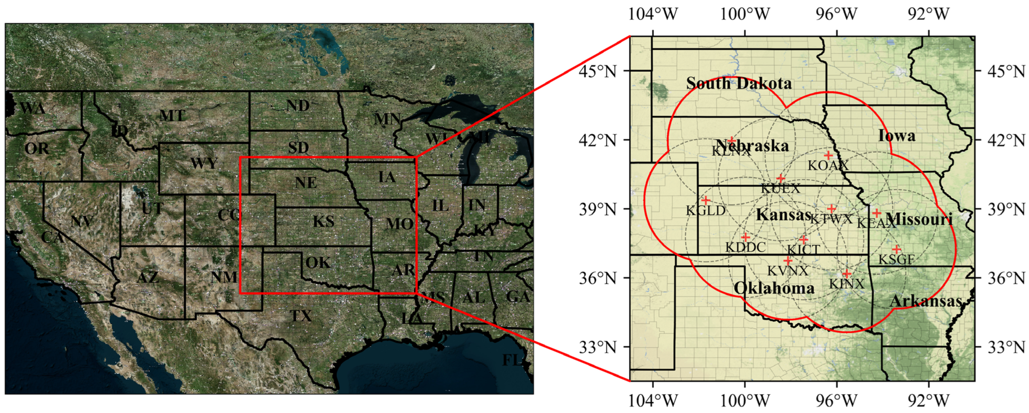Therefore, this paper initiates the following preprocessing steps for the radar data:

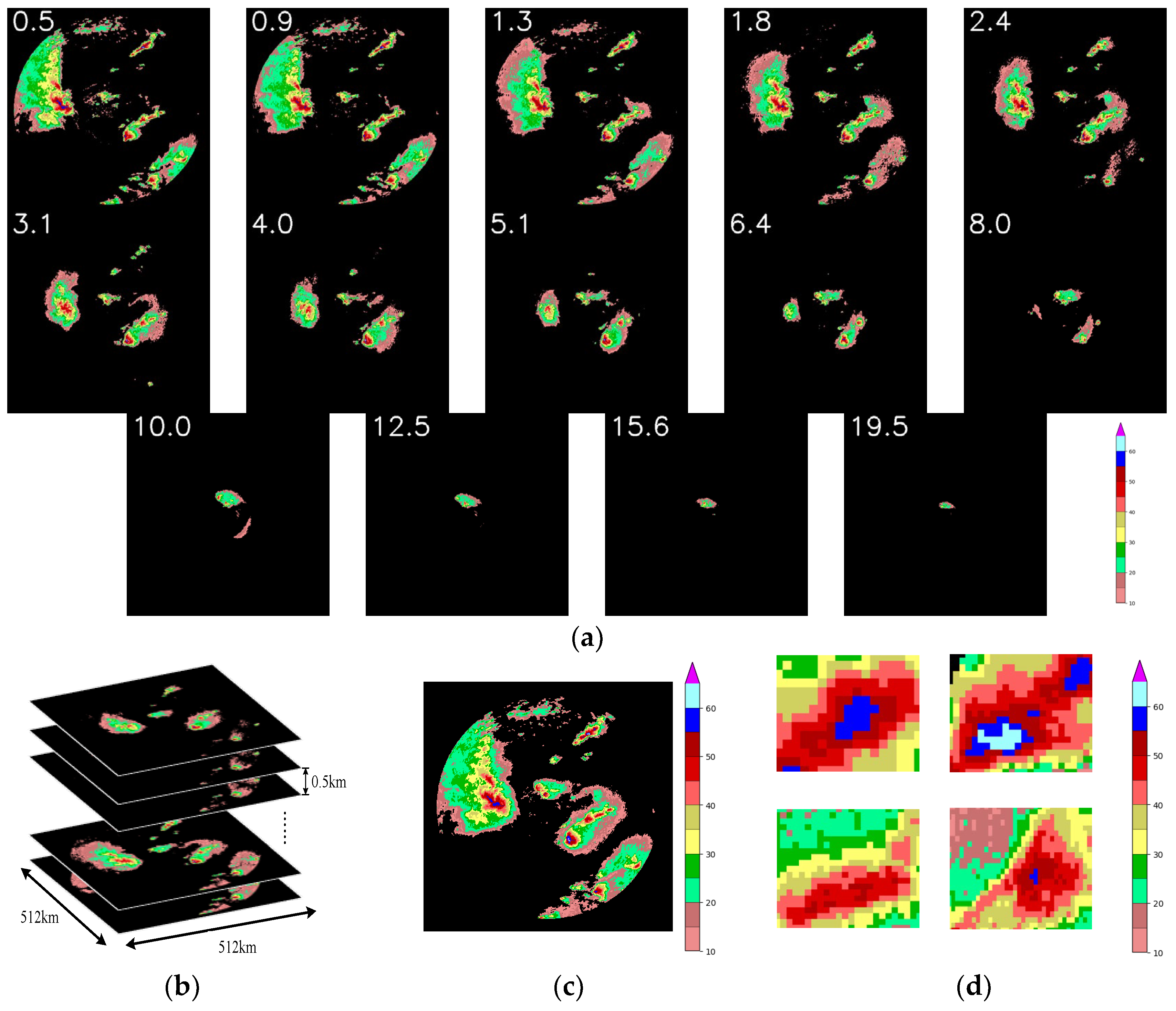
(1)

The original base data (Z_H, Z_DR, ρ_hv) were transformed into three-dimensional uniform grid format data using a bilinear interpolation algorithm;

(2)

The composite reflectivity (CR) map was generated from three-dimensional uniform grid reflectivity data using an extremum extraction algorithm [31];

(3)

The convective cells were segmented on the CR images using a flood-fill algorithm with 40 dBZ as the threshold [32], resulting in the creation of individual cell masks. Subsequently, other dual-pol data for these cells were obtained.

Figure 2b–d sequentially illustrates the results of the Z_H data after the aforementioned three-step data preprocessing.

Hail observations were obtained from January 2013 to June 2019 in Kansas. Among the data collected from the 11 radar stations depicted in Figure 2, a total of 6273 hail events and 8046 non-hail events were obtained. From these, 5273 hail events and 6546 non-hail events were randomly selected for the analysis of feature effectiveness and for training and validating the model. The remaining 1000 hail events and 1500 non-hail events were reserved for model testing.

3. Method

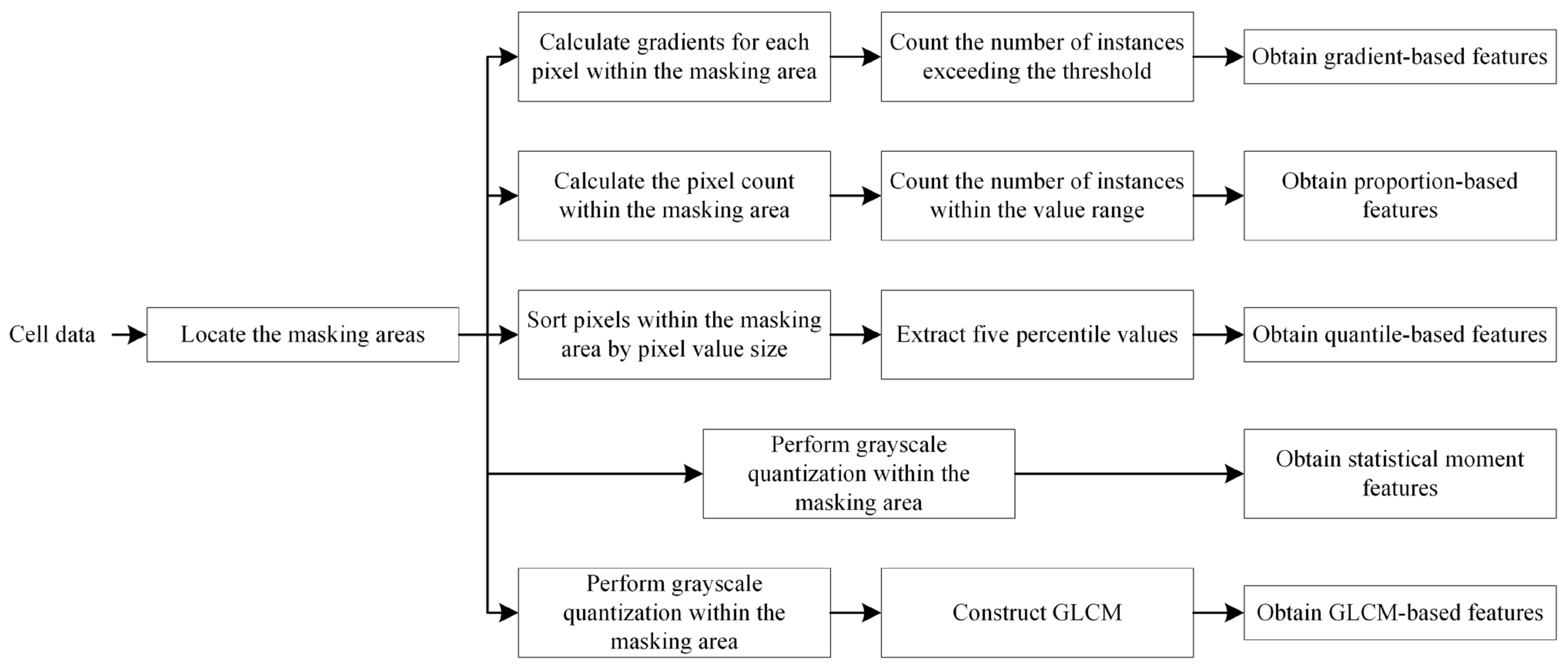
3.1. Mechanism Feature Construction Based on Fine-Grained Cell Data Distribution Details

Convective cells often exhibit larger water particle sizes and higher densities, resulting in relatively strong to extremely strong radar Z_H echoes. These features are comparatively easier to identify on CR images. In contrast to non-hail convective cells, hail-producing cells tend to display stronger Z_H with higher tops in the strong Z_H region. They often exhibit an overhanging morphology with weak echo regions, or even well-defined weak echo regions [33], owing to stronger updrafts and higher near-surface moisture saturation. Leveraging these features of hail-producing cells, this study proposes the construction of five novel mechanism features for hail identification, capitalizing on the distinctive attributes of dual-pol radar data. These features focus on the fine-grained pixel value distributions within cells. A flowchart that sets out the overall process of feature construction is presented in Figure 3. The details of the symbols mentioned in this section are shown in Appendix A,

Table A1. Glossary of notations.

Symbol	Meaning
Ω40, Ω50	The core masking areas within the CR images using respective lower threshold values of 40 dBZ and 50 dBZ
pi	The neighborhood point of pixel (x, y)
M	The mask used to calculate the feature
th, thCR, thZH, thZDR	The threshold used to calculate the feature
Gradxy	The gradient at pixel (x, y)
(x, y)∈A	$A=\left\{\left(x,y\right)|M^{\left(x,y\right)}=1\right\}$, (x, y) is the point within the mask M
hi	The height level where (x, y) is located
ω, ωCR, ωZH, ωZDR, ωρhv	The value range intervals of various data types
N40, N50	The pixel count within the masking areas Ω40 and Ω50
L	Gray level
ΩZDR	The collection of all points within the ZDR column
H(x, y, z)	The height of point (x, y, z)

.

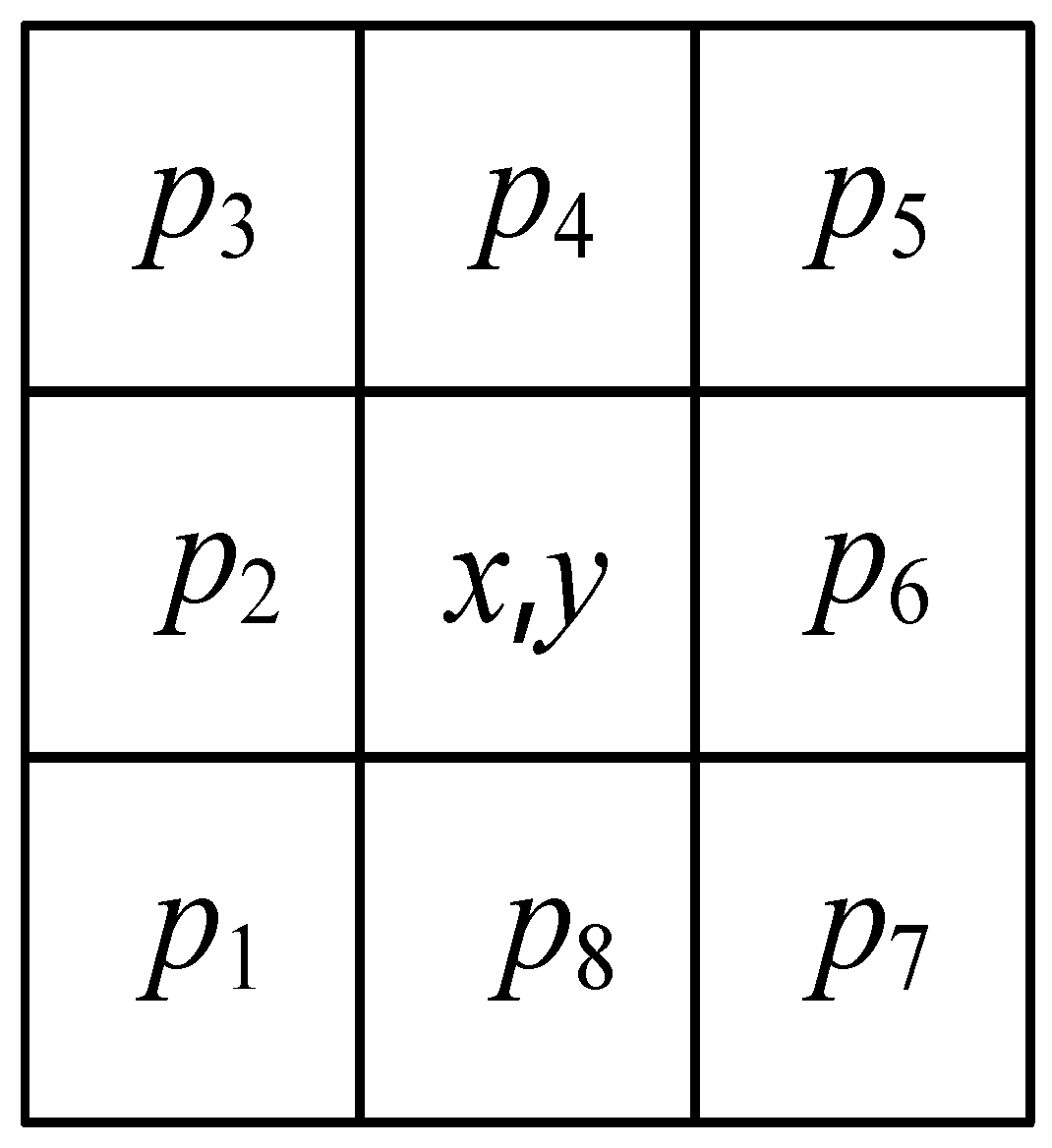
3.1.1. Gradient-Based Features

In Z_H images, convective cells typically exhibit a data distribution pattern characterized by a high-value core surrounded by a gradual decrease in values. Strong updrafts often lead to rapid changes in Z_H intensity on one side of the core to the boundary within developing hail-producing cells, while the change is slower on the other side [24,34]. In contrast, this disparity in Z_H change is less pronounced in short-duration heavy precipitation cells without hail. This indicates the presence of high-gradient values in the Z_H data within hail cell areas.

Furthermore, irregularly shaped hail particles tend to roll continuously during their descent, resulting in Z_DR values around 0 dB [35]. In contrast, raindrops falling through the air experience a flattening effect due to air resistance, leading to larger observed Z_DR values. Consequently, within the region of hail cells containing both solid- and liquid-phase water particles, local high gradients in the Z_DR data are expected to be higher than those in non-hail cells consisting solely of liquid-phase water particles. Therefore, the steps for extracting high-dimensional micro-features of high gradients within individual cells are as follows:

Step 1: Locate the core masking areas Ω₄₀ and Ω₅₀ within the CR images using respective lower threshold values of 40 dBZ and 50 dBZ.

Step 2: Calculate gradients for each pixel (x, y) within the masking area according to Equation (1) in the CR image, as well as in the Z_H images at five different height levels and the Z_DR images at five different height levels. The pixel indexing used in Equation (1) is illustrated in Figure 4, and the masking types are specified in

Table 1. Data types, masks, gradient thresholds, and dimensions for gradient-based features.

Data Type	Mask (M)	Gradient Threshold (th)	Number of Microfeatures	Dimensions of Gradient-Based Feature
CR	Ω40	2, 3, 4	3	48
ZH at 5 different heights	Ω40	2, 3, 4	3 × 5
ZDR at 5 different heights	Ω40, Ω50	1, 1.5, 2	3 × 5 × 2

. The five height levels are sequentially defined as the 0 °C layer height (H_0°C), H_0°C − 1 km, H_0°C + 1 km, the −20 °C layer height (H_−20°C), and H_−20°C − 1 km.

$${Grad}_{xy}=\mathrm{m}\mathrm{a}\mathrm{x}\left\{\left|f\left(x,y\right)-f\left(p_i\right)\right|,i=\mathrm{1,2},...,8\right\}$$

(1)

Step 3: On a per-unit basis, comprising the CR image and two-dimensional images at different height levels, count the number of instances exceeding a prescribed gradient threshold. This count is recorded as the micro-gradient feature.

Table 2. Calculation formulae for gradient-based features.

Feature Name	Calculation Formula
${\mathrm{T}\_\mathrm{G}\mathrm{r}\mathrm{a}\mathrm{d}\_\mathrm{C}\mathrm{R}}_{M,th}$	${\sum }_{\left(x,y\right)\in A}I\left({Grad}_{xy}\ge {th}_{\mathrm{C}\mathrm{R}}\right)$
${\mathrm{T}\_\mathrm{G}\mathrm{r}\mathrm{a}\mathrm{d}\_\mathrm{Z}\mathrm{H}}_{h_i,M,th}$	${\sum }_{\left(x,y\right)\in A}I\left({Grad}_{xy}\ge {th}_{\mathrm{Z}\mathrm{H}}\right)$
${\mathrm{T}\_\mathrm{G}\mathrm{r}\mathrm{a}\mathrm{d}\_\mathrm{Z}\mathrm{D}\mathrm{R}}_{h_i,M,th}$	${\sum }_{\left(x,y\right)\in A}I\left({Grad}_{xy}\ge {th}_{\mathrm{Z}\mathrm{D}\mathrm{R}}\right)$

presents the specific calculation formulas for gradient-based features.

In the equation $A=\left\{\left(x,y\right)|M^{\left(x,y\right)}=1\right\}$, M represents the applied mask, and the meanings of h_i are illustrated in

Table 3. Meanings of h_i.

hi
h1	h2	h3	h4	h5
H0°C − 1 km	H0°C	H0°C + 1 km	H−20°C − 1 km	H−20°C

. I(x) denotes the indicator function, which takes a value of 1 when x is true and 0 otherwise. The gradient threshold parameter, th, and the total dimensions of acquired gradient-based features are detailed in Table 1.

3.1.2. Proportion-Based Features in a Specified Value Range

Firstly, as the size of hydrometeor particles within the meteorological target area increases, the Z_H values detected by weather radar increase accordingly. Several statistical analyses have shown that convective cells with Z_H components of 55 dBZ and higher are more likely to trigger hail [36]. Secondly, the sensitivity of dual-pol radar’s Z_DR to hydrometeor morphology, along with the irregular spherical shape of hailstones and the flattened shape of raindrops, results in varying Z_DR values depending on the shape of hydrometeor particles. Thirdly, in general, high-altitude pure hail tends to produce high values of ρ_hv provided by dual-pol radar. However, the presence of wet hail can lower the values of ρ_hv. Therefore, ρ_hv aids in distinguishing between pure rain, hail, and mixed hail–rain components within the individual cells.

This paper designates value ranges for Z_H data, Z_DR data, and ρ_hv data obtained from dual-pol radar. Within the individual cell masking area (Ω₄₀ or Ω₅₀), it calculates the proportion of values falling within the specified ranges, thus generating ‘Proportion-Based Features in a Specified Value Range’. To capture more discriminative features, this study defines multiple specified value range intervals (ω) and masking types for each of the three dual-pol radar data, as shown in

Table 4. Data types, range intervals, masks, and such feature dimensions that form the proportion-based features in a specified value range.

Data Type	Value Range (ω)				Mask	Feature Dimension 72
CR	[45, ∞)		[55, ∞)		Ω40	2
ZH at 5 heights	[45, ∞)		[55, ∞)		Ω40	2 × 5 = 10
ZDR at 5 heights	[−0.5, 0.5]	[−1, 1]		[−1.5, 1.5]	Ω40, Ω50	5 × 3 × 2 = 30
ρhv at 5 heights	[0.85, 0.92]	[0.83, 0.94]		[0.8, 0.97]	Ω40, Ω50	5 × 3 × 2 = 30

, where the meanings of masking areas Ω₄₀ and Ω₅₀ are as described earlier. The steps for obtaining proportion-based features in a specified value range within individual cells are outlined as follows:

Step 1: Calculate the pixel count within the masking areas Ω₄₀ and Ω₅₀ on the CR image using lower threshold values of 40 dBZ and 50 dBZ, denoted as N₄₀ and N₅₀, respectively.

Step 2: Calculate the proportion-based features within the specified value ranges using data from the CR image and two-dimensional images of Z_H, Z_DR, and ρ_hv at five height levels, all within the masking area, as specified in

Table 5. Formulae for calculating the proportion-based features in a specified value range.

Feature Name	Calculation Formula
${\mathrm{T}\_\mathrm{R}\mathrm{a}\mathrm{t}\mathrm{i}\mathrm{o}\_\mathrm{C}\mathrm{R}}_{M,\omega }$	$\frac{{\sum }_{\left(x,y\right)\in A}I\left(f\left(x,y\right)\in {\omega }_{\mathrm{C}\mathrm{R}}\right)}{N_{\Omega }}$
${\mathrm{T}\_\mathrm{R}\mathrm{a}\mathrm{t}\mathrm{i}\mathrm{o}\_\mathrm{Z}\mathrm{H}}_{h_i,M,\omega }$	$\frac{{\sum }_{\left(x,y\right)\in A}I\left(f\left(x,y\right)\in {\omega }_{\mathrm{Z}\mathrm{H}}\right)}{N_{\Omega }}$
${\mathrm{T}\_\mathrm{R}\mathrm{a}\mathrm{t}\mathrm{i}\mathrm{o}\_\mathrm{Z}\mathrm{D}\mathrm{R}}_{h_i,M,\omega }$	$\frac{{\sum }_{\left(x,y\right)\in A}I\left(f\left(x,y\right)\in {\omega }_{\mathrm{Z}\mathrm{D}\mathrm{R}}\right)}{N_{\Omega }}$
${\mathrm{T}\_\mathrm{R}\mathrm{a}\mathrm{t}\mathrm{i}\mathrm{o}\_\mathsf{\rho }\mathrm{h}\mathrm{v}}_{h_i,M,\omega }$	$\frac{{\sum }_{\left(x,y\right)\in A}I\left(f\left(x,y\right)\in {\omega }_{\rho \mathrm{h}\mathrm{v}}\right)}{N_{\Omega }}$

.

In the equation, A, M, and h_i have the same meanings as in the gradient-based features. f(x, y) represents the datum value at point (x, y), while ω denotes the value range intervals corresponding to various data types, with specific values as shown in Table 4. The total dimensions of the proportion-based features in a specified value range are detailed in Table 4.

3.1.3. Quantile-Based Intensity Features

The intensity of Z_H is positively correlated with the strength of meteorological targets and serves as the most direct piece of data for assessing the strength of convective cells. Conversely, the Z_DR and ρ_hv coefficients are negatively correlated with hail events, meaning that lower values indicate a higher likelihood of hail [37,38]. Therefore, this paper directly utilizes different quantile data from three categories of data at various height levels within individual cells as intensity-based features. Additionally, for the data related to Z_DR and ρ_hv, due to the potential presence of significant value disparities within two-dimensional data at fixed height levels, the range (the difference between maximum and minimum intensity values) is incorporated as a feature. The specific extraction algorithm steps are outlined as follows:

Step 1: Locate the core masking areas Ω₄₀ and Ω₅₀ within the CR images and sort pixels within the masking areas in various data images by pixel value size.

Step 2: Extract five percentile values from the CR image and two-dimensional images of Z_H, Z_DR, and ρ_hv at five height levels. In addition, calculate the range of values for Z_DR images and ρ_hv images, which are directly employed as percentile-based intensity-class features.

The dimensions of the obtained percentile-based intensity features and the meanings of the five percentiles are summarized in

Table 6. Data types, quantiles, masks, and dimensions of quantile-based intensity features.

Data Type	Percentile (x%)	Mask	Feature Dimensions 140
CR	1%, 25%, 50%, 75%, 100%	Ω40	5
ZH at 5 heights	1%, 25%, 50%, 75%, 100%	Ω40	5 × 5 = 25
ZDR at 5 heights	1%, 25%, 50%, 75%, 100%	Ω40, Ω50	5 × 5 × 2 + 5 = 55
ρhv at 5 heights	1%, 25%, 50%, 75%, 100%	Ω40, Ω50	5 × 5 × 2 + 5 = 55

, with their definitions provided in

Table 7. The meanings of percentiles in Table 6.

x%	1%	25%	50%	75%	100%
Meaning	Minimum value	Low quartile point	Median	High quartile point	Maximum value

.

3.1.4. Statistical Moment Features Based on the Gray-Level Histogram

The statistical moments of the grayscale histogram [39] are a category of statistical analysis methods used to describe image texture features, which can be employed to express features such as the roughness/smoothness and symmetry of the image.

In order to quantify the differences in intensity distribution, roughness, and skewness of two-dimensional data images of hail and non-hail cells, this study first converts the dual-pol radar Z_H, Z_DR, and ρ_hv images into grayscale using the quantification scheme outlined in

Table 8. Data type, gray level, and data classification for generating statistical moment features.

Data Type	Gray Level L and Data Range
	l = 0	l = 1	l = 2	l = 3	l = 4	l = 5	l = 6	l = 7
CR	[34, 40)	[40, 45)	[45, 50)	[50, 55)	[55, 60)	[60, 65)	≥65
ZH at 5 heights
ZDR at 5 heights	[−3, −2)	[−2, −1)	[−1, 0)	[0, 1)	[1, 2)	[2, 3)	[3, 4)	≥4
ρhv at 5 heights	[0.4, 0.5)	[0.5, 0.6)	[0.6, 0.7)	[0.7, 0.8)	[0.8, 0.9)	≥0.9

.

Subsequently, grayscale histograms are generated for each grayscale level in the cell images under the mask region Ω₄₀, and the first-order, second-order, and third-order moments of the data are computed. The dimensions of the statistical moment features based on the grayscale histogram are presented in

Table 9. Data type, mask area, and total dimension of statistical moment features based on the gray-level histogram.

Data Type	Mask	Feature Dimensions 48
CR	Ω40	3
ZH at 5 heights	Ω40	5 × 3 = 15
ZDR at 5 heights	Ω40	5 × 3 = 15
ρhv at 5 heights	Ω40	5 × 3 = 15

.

3.1.5. Features Based on the Gray-Level Co-occurrence Matrix

The gray-level co-occurrence matrix (GLCM) of an image describes the joint probability distribution of pixel pairs with a certain distance and angular relationship in the image. It is used to reflect the spatial distribution patterns of grayscale values in the image, specifically, it reflects the grayscale distribution information of the image in a particular direction and distance [40]. This approach belongs to the category of statistically based methods for extracting texture features from images.

A grayscale image F with L (0, 1, 2, …, L − 1) gray levels has a GLCM that is an L × L square matrix. The elements of this matrix, denoted as g_ij (i, j = 0, 1, 2, …, L − 1), represent the probability of a specified pixel pair occurring at a designated position in the image. The value of gij is equal to the ratio of pixel pairs meeting the conditions f(p₁) = i and f(p₂) = j along the θ direction with a separation of r in the image, where r = 1, and θ is set to 0°, 45°, 90°, and 135° in this study.

To begin with, the grayscale processing is applied to the CR image, Z_H images, Z_DR images, and ρ_hv images under the cell mask region Ω₄₀. The grayscale levels and their corresponding data intervals are detailed in Table 8. Following this, 64 GLCMs are constructed from these 16 grayscale images (1 + 5 × 3 = 16) for the four θ. Subsequently, texture features, including contrast ratio, energy, entropy, and inverse variance [41], typically used to represent image texture features, are extracted. The overall dimensionality of the features based on the GLCM is 256 (64 × 4).

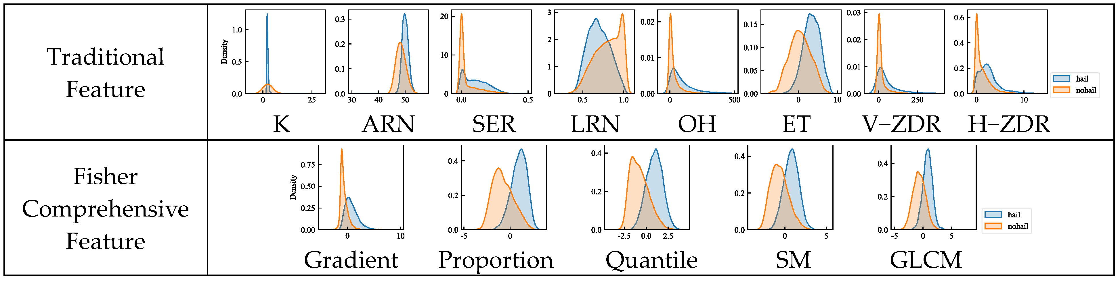
3.2. Construction of Traditional Mechanism-Based Features

To evaluate the effectiveness of the newly constructed hail mechanism-based features in this study, we conducted a comparative analysis with traditional mechanism-based features. In accordance with meteorological forecasting experience and our previous research efforts, we selected six mechanism features [24,42] based on Z_H images and the Z_DR column feature [27] based on Z_DR images as representatives of traditional mechanism-based features. Each feature is described as follows:

(1)

Kurtosis (K) [24]: Kurtosis is a fourth-order statistical measure based on histogram data from images, used to quantify the steepness of the peak in the histogram. Compared to non-hail cells, hail cells (regions with Z_H of 40 dBZ and higher) have a higher proportion of high Z_H values. Therefore, typically, the intensity distribution histogram of non-hail cells has a steeper peak;

(2)

Average reflectivity of nucleus (ARN) [42]: ARN is defined as the reflectivity-weighted average within contiguous regions on a radar CR image where the Z_H exceeds or equals 45 dBZ. A higher ARN indicates a greater likelihood of hail precipitation;

(3)

Strong echo ratio (SER) [24]: SER is used to describe the proportion of strong echoes above the −20 °C level and serves as a quantitative measure of the intense echo signals at higher altitudes;

(4)

Liquid ratio of nucleus (LRN) [42]: LRN is the feature specifically designed for hail identification on the basis of vertical integrated liquid water content (VIL). As cells pass through the freezing level, precipitation particles gradually transition from a liquid to a solid state (such as ice crystals). The reflectivity values of substances like ice crystals within hail clouds do not conform to their empirical relationship with liquid water. By establishing an attenuation coefficient, LRN attenuates liquid water content converted from the reflectivity, calculating the density of weighted vertical integrated liquid water content. This plays a significant role in distinguishing between hail and short-duration heavy rainfall events;

(5)

Effective thickness (ET) [42]: Severe hail-producing weather is more likely to occur with higher and more intense updraft. Effective thickness is a quantitative measure of this phenomenon;

(6)

Overhang (OH) [24]: Cells with the potential for hail exhibit an overhanging pattern, where the Z_H structure at lower levels displays strong echoes suspended above weaker echo bodies. The presence of low-level moisture-carrying strong updrafts is a primary contributor to the weaker echo regions. Hence, the size of the weaker echo body volume can be used to quantitatively measure the intensity of the updraft, defining overhang in terms of the volume of the weaker echo region;

(7)

Volume and Height of Z_DR Column

The interpretation of Z_DR data provided by dual-pol radar determines the capacity of Z_DR values to carry phase information about detected hydrometeors. For instance, Z_DR values greater than or equal to 1 dB typically indicate the presence of liquid-phase water particles. In contrast, water particles situated above the 0 °C level for a period of time are often in solid form, resulting in Z_DR values around 0 dB.

The updraft within convective cells transports liquid water from the lower atmosphere into layers above the 0 °C level. Consequently, a water column appears above the 0 °C level, which can be reflected in Z_DR data. Research by Snyder et al. [27] has shown that the vertical extent of the Z_DR column is related to the intensity of the strongest updraft. Thus, it can be stated that the Z_DR column of liquid water particles aggregated at and above the 0 °C level provides information about the position and intensity of updrafts within storm cells.

Because the strength of the updraft is related to the growth potential of hail, the Z_DR column can indirectly serve as an indicator of the physical and dynamic structure of hail clouds, and its variations can be used to predict the development of hail clouds [43]. In this study, based on a regional growth approach, we have redefined the algorithm for extracting Z_DR column features, focusing on two key aspects: maximum volume and maximum height.

Step 1: Regions with Z_H values equal to or exceeding 40 dBZ were extracted from the CR image and utilized as a mask to delineate the corresponding areas in the ρ_hv image and the Z_DR image;

Step 2: Within the defined areas and the three-dimensional space extending above the 0 °C level, a region-growing method was employed to obtain the Z_DR column. The collection of all points within the column is denoted as Ω_ZDR, where the growth template size is 3 × 3 × 3, and the growth criteria include Z_DR values greater than or equal to 1 dB and ρ_hv values between 0.8 and 1.

Step 3: Generate the height projection image of the Z_DR column, where the value at point (x, y) is set to $H_{\mathrm{Z}\mathrm{D}\mathrm{R}}\left(x,y\right)=\underset{z}{\max }\left\{H\left(x,y,z\right)-H_{0°\mathrm{C}}\right\}$.

As a result, height, and volume features of the Z_DR column are obtained:

$$T_{H-\mathrm{Z}\mathrm{D}\mathrm{R}}=\max H_{\mathrm{Z}\mathrm{D}\mathrm{R}}\left(x,y\right)$$

(2)

$$T_{V-\mathrm{Z}\mathrm{D}\mathrm{R}}=\sum H_{\mathrm{Z}\mathrm{D}\mathrm{R}}\left(x,y\right)$$

(3)

4. Experiment and Analysis

4.1. Feature Validity Assessment

Table 10. Summary of mechanism features of hail cell.

Type	Feature Dimensions
Gradient-based features	48	564
Proportion-based features in a specified value range	72
Quantile-based intensity features	140
Statistical moment features based on the gray-level histogram	48
Features based on the GLCM	256

presents specific dimensional information for five categories of mechanism-based features that rely on the distribution details of cell data. Due to the diversity of feature types, it is necessary to compute similar features at different height levels and under different thresholds, which can inevitably result in issues such as excessively high feature dimensionality and redundancy among certain features. To assess their effectiveness in identifying hail and non-hail cells, this section employs hypothesis testing to conduct a validity assessment of the features and remove those with low discriminative power.

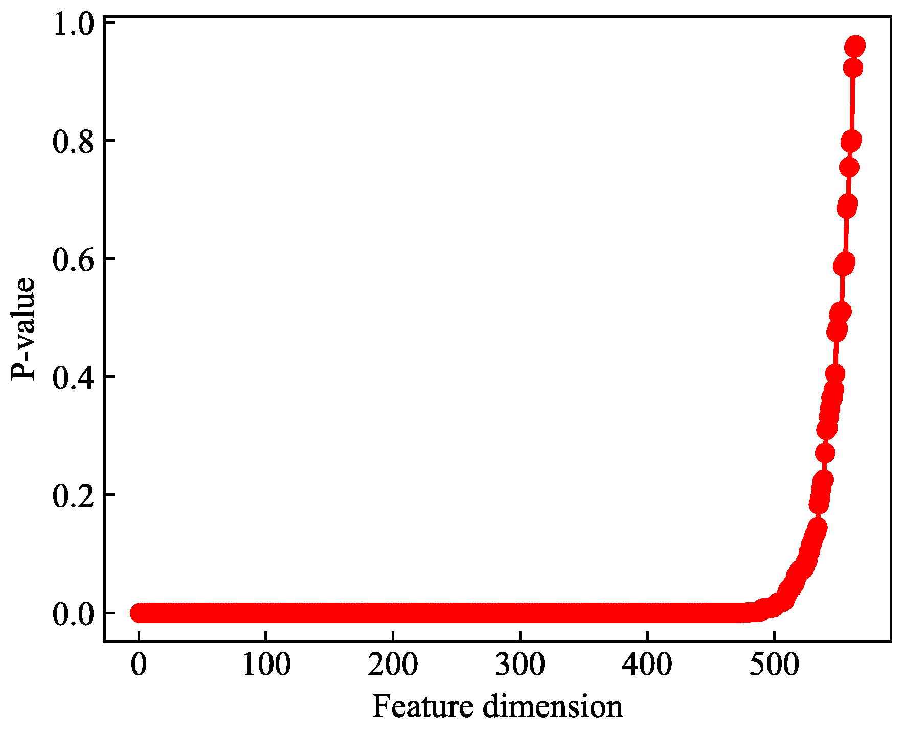
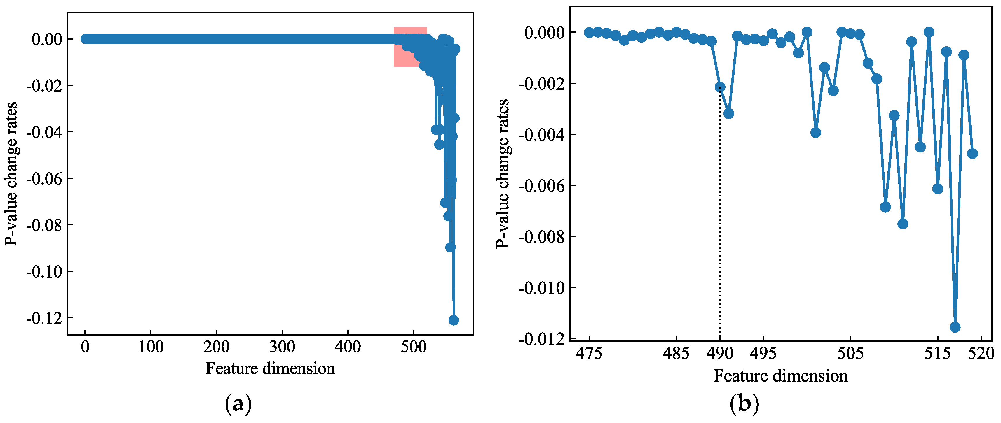
4.1.1. Hypothesis Testing Methods

Hypothesis testing initially involves formulating a hypothesis about a parameter or distribution type for a given population, and then assesses the reliability of that hypothesis by performing calculations based on sample data [44].

In this study, for the proposed features, a significance test for the difference in means between hail and non-hail cell populations is conducted using a large sample set, following the principles of the t-distribution. Within the t-distribution theory, the p-value represents the probability of making a type I error, which is the probability of falsely claiming a difference in means between the two populations [45]. A smaller p-value suggests a more pronounced difference in the distribution of the tested feature between hail and non-hail populations, indicating the suitability of this feature.

4.1.2. Hypothesis Testing Results

Following the principles of hypothesis testing, the p-values for the features are computed and then arranged in ascending order. The distribution of p-values, sorted from smallest to largest, is illustrated in Figure 5.

From Figure 5, it is evident that the p-values for approximately the first 480 features are close to 0.00 and exhibit a relatively stable distribution, while the remaining features have higher p-values with rapidly changing trends. To determine the dimensionality of the retained features, this study calculates the rate of change of p-values at each point in Figure 5. Figure 6 displays the distribution of these p-value change rates. As shown in Figure 6, the p-values for the first 490 features remain stable and close to 0.00, but a significant change occurs between the 490th and 491st features. Beyond the 490th feature, the p-values become larger, and there is noticeable fluctuation. Consequently, this paper retains the first 490 mechanism-based features and removes the remaining 74 features.

Table 11. Feature that failed the hypothesis test.

Feature Type	Data Type									Proportion
	ZH	ZDR	ρhv	CR	H0–1	H0	H0+1	H–20	H–20–1
Proportion-based	0	0	11	0	4	5	2	0	0	11/72
Quantile-based	1	18	18	0	0	13	10	8	6	37/140
Statistical moments	4	1	3	0	1	2	1	2	2	8/48
GLCM	6	8	4	0	2	1	2	7	6	18/256

provides basic information about the removed features.

The results of feature validity assessment using hypothesis testing can be summarized as follows:

(1)

Among the 564-dimensional features constructed in this study, all 48 features in the gradient category exhibit significant differences;

(2)

Among the remaining 516 (564–48) features, 74 features were removed due to excessively high p-values, indicating that these features did not demonstrate a significant difference in mean distribution between hail and non-hail cells.

From Table 11, the following observations can be made: (1) Mechanism-based features derived from the CR image exhibit significant differences between hail and non-hail cells. (2) When data is derived from higher altitude levels, features based on the specified value range are all applicable. However, for the features calculated using ρ_hv at three lower altitude levels, 11 of them do not pass the hypothesis testing. (3) Percentile features are generally more effective on Z_H images at lower altitude levels. (4) The selection rates for features in the categories of grayscale histogram statistical moments and GLCM texture features are 83% and 93%, respectively.

4.2. Hail Identification Model Construction and Test Metrics

4.2.1. Identification Model

The support vector machine (SVM) model exhibits excellent classification performance [46]. The fundamental SVM strives to find an optimal hyperplane in the feature space for linearly separable problems, ensuring that the shortest distance between modeling samples of two classes to this hyperplane is equal while maximizing it as much as possible [47]. Since its inception, SVM has been considered one of the most successful and valuable machine learning methods, widely applied and researched in hail identification [24]. In this study, we employ the SVM to establish a hail identification model based on mechanism features.

4.2.2. Testing Metrics for Identification Models

In accordance with meteorological industry conventions, the classification ability of the hail identification model is assessed using three metrics: probability of detection (POD), false alarm rate (FAR), and critical success index (CSI). Let a represent the number of hail samples correctly identified by the model, b represent the number of hail samples missed by the model, and c represent the number of non-hail samples incorrectly identified as hail by the model. The calculation formulas for these three metrics are shown in Equations (4)–(6).

POD = a/(a + b)

(4)

FAR = c/(a + c)

(5)

CSI = a/(a + b + c)

(6)

4.3. Comparison of Hail Identification Models in Two Mechanism Feature Spaces

4.3.1. Hail Identification Model Based on Traditional Mechanism Features

In the modeling sample set, 5273 hail samples and 6546 non-hail samples were randomly selected. Two hail classification identification models were developed sequentially: one based on six-dimensional features derived from Z_H and another based on six-dimensional features from Z_H combined with two-dimensional mechanistic features derived from the Z_DR column. Subsequently, the models were tested using the remaining 1000 hail and 1500 non-hail samples. The test results are presented in

Table 12. Scoring of hail identification model based on traditional mechanism features.

Model	ZH Feature	ZDR Column	POD	FAR	CSI
1	√		0.804	0.290	0.605
2	√	√	0.820	0.286	0.617

.

From Table 12, it can be observed that: (1) Consistent with previous research findings, the six-dimensional traditional mechanism features exhibit a strong discriminative ability between hail and non-hail cells [24,42]. The hail identification model established solely using the six-dimensional Z_H features achieved a commendable CSI score of 60.5%. (2) Upon the inclusion of two-dimensional Z_DR column features, the model’s POD increased by 1.6%, the FAR decreased by 0.4%, and the CSI improved by 1.2%. This indicates the positive impact of dual-pol parameters on enhancing model quality [9,48,49]. It is worth noting that dual-pol radar necessitates higher data accuracy and stability. As the calibration quality of dual-pol radar improves, the inclusion of dual-pol parameters like Z_DR may potentially yield even greater enhancement in algorithm performance.

4.3.2. Hail Identification Model Based on Mechanism Features from Cell Data Distribution Details

Using the same training samples as in the previous section, a hail identification model was constructed in the newly created 490-dimensional mechanism feature space. Subsequently, testing was performed using the set of test samples, and the test results are presented in

Table 13. Scoring of hail identification model based on the 490-dimensional mechanism features.

Model	Feature	POD	FAR	CSI
3	490-dimensional mechanism features	0.701	0.193	0.600

.

It can be observed that: (1) Compared to the hail identification model constructed based on the traditional eight-dimensional mechanism features, the model established in the newly created 490-dimensional mechanism feature space achieved slightly lower scores. It incurred a reduction of 11.9% in the POD in exchange for a decrease of 9.3% in the FAR. (2) In contrast to Model 1 in Table 12, the expected improvement in hail identification due to the inclusion of dual-pol parameters did not materialize. The following potential explanations are provided: (1) The utilization of features as high as 490 dimensions may require a larger set of training samples. (2) It is challenging for a SVM to directly induce patterns of inter-class differences from a dataset described with such high-dimensional features.

Therefore, the following two feature comprehensive methods were designed in this study:

(1)

Principal Component Analysis (PCA) [50] was used to integrate the 490-dimensional features from five different perspectives. Specifically, from the five sub-feature spaces of gradient, specified value range ratio, quantiles, grayscale histogram statistical moments, and texture based on the GLCM, the directions of maximum variance and second maximum variance were obtained, resulting in a total of 10 comprehensive features (principal components);

$$T\_PCA\_1=\left({t_{pca}}_{Grad-1},{t_{pca}}_{Ratio-1},{t_{pca}}_{x\%-1},{t_{pca}}_{SM-1},{t_{pca}}_{GLCM-1}\right)$$

(7)

$$T\_PCA\_2=\left({t_{pca}}_{Grad-2},{t_{pca}}_{Ratio-2},{t_{pca}}_{x\%-2},{t_{pca}}_{SM-2},{t_{pca}}_{GLCM-2}\right)$$

(8)

(2)

Fisher Linear Discriminant Analysis [51] was employed to integrate and reduce the dimensionality of the 490-dimensional features from five different perspectives. In each of the five sub-feature spaces, the projection direction that maximizes the criterion function of difference between inter-class means divided by sum of intra-class variances was determined, resulting in five comprehensive features.

$$T\_Fisher=\left(t_{Grad-Fisher},t_{Ratio-Fisher},t_{x\%-Fisher},t_{SM-Fisher},t_{GLCM-Fisher}\right)$$

(9)

Separately, hail identification models were trained in three feature spaces: the 5-dimensional principal component comprehensive feature space, the 10-dimensional principal component comprehensive feature space, and the 5-dimensional Fisher comprehensive feature space. Subsequently, tests were conducted on these models, and the test results are presented in

Table 14. Scoring of hail identification model based on comprehensive features of hail cell.

Model	Comprehensive Feature	POD	FAR	CSI
4	5 first principal components	0.796	0.316	0.582
5	5 first principal components + 5 s principal components	0.799	0.279	0.610
6	5 Fisher	0.867	0.278	0.650

. It can be observed that:

(1)

As the dimensionality of PCA comprehensive features increases, classifier performance improves. Furthermore, the use of the 10-dimensional PCA comprehensive feature scheme is more effective than directly building models in the 490-dimensional feature space. This aligns with our expectations and previous research findings [19,20,42];

(2)

The Fisher feature comprehensive scheme, overall, outperforms the PCA feature comprehensive scheme. This is because PCA’s “maximum variance criterion” may not necessarily align with the classification objective, while Fisher’s “intra-class cohesion, inter-class separation [52]” criterion aligns with the goals of a classification function. This further substantiates the feasibility of Fisher Linear Discriminant Analysis in hail identification [21,53];

(3)

After adopting the Fisher feature comprehensive scheme, the model based on the five-dimensional comprehensive features outperforms the traditional mechanism feature-based identification model. This strongly validates the significant effectiveness of the newly constructed five-dimensional mechanism features in hail identification, further emphasizing that dual-pol radar data can indeed enhance the quality of hail identification models. In the eight-dimensional traditional mechanism feature space, the utilization of dual-pol data is inadequate.

To gain further insight into the capability of the five-dimensional Fisher comprehensive features and the eight-dimensional traditional mechanism features in describing the two classes of modeling samples, sample distribution density plots were generated, as shown in Figure 7.

It can be observed that the discriminative ability of the five-dimensional Fisher-comprehensive mechanism features between the two sample classes is generally superior to that of traditional mechanism features. Therefore, the 3.3 percentage point higher CSI score obtained by Model 6 in Table 14 compared to Model 2 in Table 12 is expected.

4.3.3. Joint Utilization of Two Types of Mechanism Features for Hail Identification Model Construction

While it is evident that the quality of the hail identification model based on the five-dimensional Fisher-comprehensive features outperforms that of the eight-dimensional traditional features, it cannot be ruled out that the two feature spaces may complement each other in terms of information. Therefore, this paper proposes a comprehensive hail identification model based on both types of mechanism features, as illustrated in Figure 8. The test results are presented in

Table 15. Scoring of hail identification model based on mechanism features of hail cell.

Model	Sample Description Method	POD	FAR	CSI
1	8-dimensional traditional mechanism features	0.820	0.286	0.617
2	5-dimensional Fisher-comprehensive features	0.867	0.278	0.650
3	8-dimensional traditional mechanism features +5-dimensional Fisher-comprehensive features	0.865	0.275	0.651

. For ease of comparison, the table includes the test results of Model 2 from Table 12 and Model 6 from Table 14 in the first two rows. It can be observed that:

(1)

Combining the five-dimensional Fisher-comprehensive features of the second-class mechanism features with the first-class mechanism features (traditional, eight-dimensional) indeed improves the hail identification model’s scores;

(2)

Comparing the three models in Table 15, it is evident that among the 13-dimensional features used to describe samples, the 5-dimensional Fisher-comprehensive features play an overwhelmingly dominant role. In terms of the difficulty level of feature extraction, constructing the eight-dimensional traditional feature extraction algorithm is more challenging than the latter. This is because the former requires a deeper understanding of the overall morphology and structure of hail clouds, as well as the ability to summarize and generalize, along with precise algorithmic representation capabilities. In contrast, the latter only needs to internalize the understanding of hail formation mechanisms into determining data height layers, partitioning data value ranges, and setting thresholds. The extraction of micro-gradient operators, specified value range ratios, quantiles, grayscale histogram statistical moments, and texture feature calculation methods based on the GLCM are all generic and convenient. Therefore, its technical threshold is much lower than that of the former. When using the Fisher method to integrate the corresponding sub-feature classes, it is possible to obtain high-quality hail identification models in a lower-dimensional comprehensive feature space.

5. Conclusions

This paper utilizes dual-pol radar data to address the structural features of hailstorms. It introduces methods for constructing five categories of hailstorm features and employs machine learning techniques to develop a hail identification model. The study validates the feasibility of the feature construction method. The specific conclusions are as follows:

(1)

The addition of dual-pol data, specifically Z_DR and ρ_hv, to the hail identification model has led to an improvement of nearly five percentage points in the CSI test results. This demonstrates a clear and significant enhancement in the quality of the hail identification model when utilizing dual-pol data;

(2)

In the face of five types of high-dimensional feature spaces, Fisher linear discriminant analysis is used to obtain comprehensive features of each category, and this method of feature construction is proven to be feasible and beneficial. The CSI score of the hail identification model based on 5-dimensional features is 0.65, which is five percentage points higher than that of the model based on 490-dimensional features;

(3)

The construction of traditional mechanism features requires algorithm designers to have a profound understanding of the phenomena and essence of the research object and to be able to scientifically incorporate the phenomena and essence of the research object into the algorithms. This approach has a high technical threshold. In contrast, the computational methods for the features proposed in this study are both versatile and easily implementable. When combined with appropriate feature comprehensive techniques, they can achieve higher quality results. Leveraging machine learning methods, it becomes possible to achieve hail identification in a low-dimensional comprehensive feature space.

This study also has certain limitations. The hail and non-hail sample data used in this research were sourced from the dual-pol radar in the United States, requiring adaptation and testing of this method when ample data from dual-pol radars in our country become available. Furthermore, our focus will next be on assessing the identification efficacy of these features in distinguishing between hail and short-duration heavy rainfall events. Additionally, we will examine their classification performance across various hail cloud types and continuously refine our feature construction methodology.

References

- Yang, X. Hail Identification and Forecasting Method Based on Dual Polarization Radar; School of Electrical and Information Engineering, Tianjin University: Tianjin, China, 2021. [Google Scholar]
- Zhong, C.; Zhang, Y.; Gao, J.Q.; Lin, J.J.; Zheng, K. Application of dual polarization doppler weather radar in hail identification. Guangdong Meteorol. 2014, 36, 76–80. [Google Scholar]
- Hand, W.H.; Cappelluti, G. A global hail climatology using the UK Met Office convection diagnosis procedure (CDP) and model analyses. Meteorol. Appl. 2011, 18, 446–458. [Google Scholar] [CrossRef]
- Cao, Y.C.; Tian, F.Y.; Zheng, Y.G.; Sheng, J. Statistical characteristics of environmental parameters for hail over the two-step terrains of China. Plateau Meteorol. 2018, 37, 185–196. [Google Scholar]
- Zhao, J.T.; Yue, Y.J.; Wang, J.A.; Yin, Y.Y.; Feng, H.Y. Study on spatio temporal pattern of hail disaster in China mainland from 1950 to 2009. Chin. J. Agrometeorol. 2015, 36, 83–92. [Google Scholar]
- Li, X.F.; Zhang, Q.H.; Zou, T.; Lin, J.P.; Kong, H.; Ren, Z.H. Climatology of hail frequency and size in China, 1980–2015. J. Appl. Meteorol. Climatol. 2018, 57, 875–887. [Google Scholar] [CrossRef]
- Guan, Y.; Zheng, F.; Zhang, P.; Qin, C. Spatial and temporal changes of meteorological disasters in China during 1950–2013. Nat. Hazards 2015, 75, 2607–2623. [Google Scholar] [CrossRef]
- Yu, X.; Zheng, Y. Advances in severe convection research and operation in China. J. Meteorol. Res. 2020, 34, 189–217. [Google Scholar] [CrossRef]
- Wu, C.; Liu, L.; Liu, X.; Li, G.; Chen, C. Advances in Chinese dual-polarization and phased-array weather radars: Observational analysis of a supercell in southern China. J. Atmos. Ocean. Technol. 2018, 35, 1785–1806. [Google Scholar] [CrossRef]
- Yu, X.D. Detection and warnings of severe convection with Doppler weather radar. Adv. Meteor. Sci. Technol. 2011, 1, 31–41. [Google Scholar]
- Doviak, R.J.; Zrnic, D.S. Doppler Radar and Weather Observations, 2nd ed.; Dover Publications: Mineola, NY, USA, 1993. [Google Scholar]
- Bringi, V.N.; Chandrasekar, V. Polarimetric Doppler Weather Radar: Principles and Applications; Cambridge University Press: Cambridge, UK, 2001. [Google Scholar]
- Zhang, G.F. Weather Radar Polarimetry; CRC Press: Boca Raton, FL, USA, 2016. [Google Scholar]
- Tang, M.H.; Yu, X.D.; Wang, Q.X.; Wang, Q.H.; Hu, M. Analysis on environmental conditions and dual-polarization radar characteristics of the phase transformation of precipitation in a rain and snow event in Hunan. Torrential Rain Disasters 2023, 42, 293–302. [Google Scholar]
- Waldvogel, A.; Federer, B.; Grimm, P. Criteria for the detection of hail cells. J. Appl. Meteorol. 1979, 18, 1521–1525. [Google Scholar] [CrossRef]
- Greene, D.R.; Clark, R.A. Vertically integrated liquid water—A new analysis Tool. Am. Meteorol. Soc. 1972, 100, 522–548. [Google Scholar] [CrossRef]
- Amburn, S.A.; Wolf, P.L. VIL density as a hail indicator. Am. Meteorol. Soc. 1997, 12, 476–478. [Google Scholar] [CrossRef]
- Manzato, A. Hail in northeast Italy: A neural network ensemble forecast using sounding-derived indices. Weather Forecast. 2013, 28, 3–28. [Google Scholar] [CrossRef]
- Zhang, Y.; Ji, Z.; Xue, B.; Wang, P. A novel fusion forecast model for hail weather in plateau areas based on machine learning. J. Meteorol. Res. 2021, 35, 896–910. [Google Scholar] [CrossRef]
- Wang, P.; Shi, J.Y.; Hou, J.Y.; Hu, Y. The identification of hail storms in the early stage using time series analysis. J. Geophys. Res. Atmos. 2018, 123, 929–947. [Google Scholar] [CrossRef]
- López, L.; Sánchez, J.L. Discriminant methods for radar detection of hail. Atmos. Res. 2009, 93, 358–368. [Google Scholar] [CrossRef]
- Blair, S.F.; Deroche, D.R.; Boustead, J.M.; Leighton, J.W.; Barjenbruch, B.L.; Gargan, W.P. A radar-based assessment of the detectability of giant hail. Electron. J. Sev. Storms Meteorol. 2011, 6, 1–30. [Google Scholar] [CrossRef]
- Skripniková, K.; Řezáčová, D. Radar-based hail detection. Atmos. Res. 2014, 144, 175–185. [Google Scholar] [CrossRef]
- Wang, P.; Pan, Y. Recognition model of heavy hail based on salient features. J. Phys. 2013, 62, 515–524. [Google Scholar]
- Zhou, K.H.; Zheng, Y.G.; Li, B.; Dong, W.S.; Zhang, X.L. Forecasting different types of convective weather: A deep learning approach. J. Meteorol. Res. 2019, 33, 797–809. [Google Scholar] [CrossRef]
- Kumjian, M.R.; Ryzhkov, A.V. Polarimetric Signatures in Supercell Thunderstorms. J. Appl. Meteor. Clim. 2008, 47, 1940–1961. [Google Scholar] [CrossRef]
- Snyder, J.C.; Ryzhkov, A.V.; Kumjian, M.R.; Khain, A.P.; Picca, J. A Z(DR) column detection algorithm to examine convective storm updrafts. Am. Meteorol. Soc. 2015, 30, 1819–1844. [Google Scholar]
- Dawson, D.T.; Mansell, E.R.; Kumjian, M.R. Does wind shear cause hydrometeor size sorting? J. Atmos. Sci. 2015, 72, 340–348. [Google Scholar] [CrossRef]
- Broeke, V.D.; Matthew, S. Polarimetric variability of classic supercell storms as a function of environment. J. Appl. Meteorol. Clim. 2016, 55, 1907–1925. [Google Scholar] [CrossRef]
- Zhang, C.; Wang, H.; Zeng, J.; Ma, L.; Guan, L. Short-term dynamic radar quantitative precipitation estimation based on wavelet transform and support vector machine. J. Meteorol. Res. 2020, 34, 413–426. [Google Scholar] [CrossRef]
- Yu, X.D.; Yao, X.P.; Xiong, T.N.; Zhou, X.G.; Wu, H.; Deng, B.S.; Song, Y. Principle and Operational Application of Doppler Weather Radar; China Meteorological Press: Beijing, China, 2006. [Google Scholar]
- Wang, P.; Li, C.; Zhang, Y. An adaptive segmentation arithmetic adapted to intertwined irregular convective storm images. In Proceedings of the 2013 International Conference on Machine Learning and Cybernetics, Tianjin, China, 14–17 July 2013; pp. 896–900. [Google Scholar]
- Shi, J.; Wang, P.; Wang, D.; Jia, H. Radar-Based Automatic Identification and Quantification of Weak Echo Regions for Hail Nowcasting. Atmosphere 2019, 10, 325. [Google Scholar] [CrossRef]
- Baeck, M.L.; Smith, J.A. Rainfall estimation by the WSR-88D for heavy rainfall events. Weather Forecast. 1998, 13, 416–436. [Google Scholar] [CrossRef]
- Miller, L.J.; Tuttle, J.D.; Knight, C.A. Airflow and hail growth in a severe northern high plains supercell. J. Atmos. Sci. 2010, 45, 736. [Google Scholar] [CrossRef]
- Mason, B.J. Physics of Clouds; Clarendon Press: Cary, NC, USA, 2010. [Google Scholar]
- Diao, X.G.; Li, F.; Wan, F.J. Comparative analysis on dual polarization features of two severe hail supercells. J. Appl. Meteor. Sci. 2022, 33, 414–428. [Google Scholar]
- Kumjian, M.R. Principles and Applications of Dual-Polarization Weather Radar. Part I: Description of the Polarimetric Radar Variables. J. Oper. Meteorol. 2013, 1, 226–242. [Google Scholar] [CrossRef]
- Lu, L.J.; Liu, Z.W.; Yang, T.; Chen, Y.C. Grayscale histogram and texture features of wake vortex image behind circular cylinder. J. Hydroelectr. Eng. 2022, 41, 1–11. [Google Scholar]
- Huang, F.H.; Li, X.C.; Wang, K.; Chao, Y.; Liang, D. Diode character recognition based on gray level co-occurrence matrix texture features and MLP. J. Jiangsu Univ. Technol. 2023, 29, 64–71. [Google Scholar]
- Li, Z.F.; Zhu, G.C.; Dong, T.F. Application of GLCM-based texture features to remote sensing image classification. Geol. Explor. 2011, 47, 456–461. [Google Scholar]
- Li, C. Research on Severe Hail Automatic Identification and Hail Suppression Decision Technology; School of Electrical and Information Engineering, Tianjin University: Tianjin, China, 2014. [Google Scholar]
- Shen, Y.; Zhou, Y.J.; Zou, S.P.; Yang, Z.; Zeng, Y. Analysis of evolution characteristics of “ZDR column” in an isolated hail storm. Meteorol. Sci. Technol. 2023, 51, 104–114. [Google Scholar]
- Wang, Z.F.; Pan, X.; Jin, S.; Tian, F.; Wang, Y. Hypothetical testing principles and application. J. Bohai Univ. Nat. Sci. Ed. 2013, 34, 101–105. [Google Scholar]
- Huang, S.; Jiang, Q.Q.; Wang, S.Q.; Cao, S.Y. P-value and confidence interval: Connection and difference, misuse and argument. J. Math. Med. 2023, 36, 3–8. [Google Scholar]
- Pan, H.C.; Luo, D.L.; Xu, B.Q. Research on radar target recognition based on doppler spectrum characteristics. Fire Control Radar Technol. 2023, 52, 50–55. [Google Scholar]
- Feng, Z.L.; Xiao, H.Q.; Ren, W.F.; Du, Y.L. Transformer fault diagnosis based on principal component analysis and seagull optimization support vector machine. China Meas. Test 2023, 49, 99–105. [Google Scholar]
- Kumjian, M.R.; Prat, O.P.; Reimel, K.J.; Van Lier-Walqui, M.; Morrison, H.C. Dual-polarization radar fingerprints of precipitation physics: A review. Remote Sens. 2022, 14, 3706. [Google Scholar] [CrossRef]
- Zhao, K.; Huang, H.; Wang, M.G.; Lee, W.C.; Chen, G.; Wen, L.; Wen, J.; Zhang, G.F.; Xue, M.; Yang, Z.W.; et al. Recent progress in dual-polarization radar research and applications in China. Adv. Atmos. Sci. 2019, 36, 961–974. [Google Scholar] [CrossRef]
- Cui, M.L.; Wang, Y.J. Vulnerability analysis of grid event region based on principal component analysis. Geomat. Spat. Inf. Technol. 2023, 46, 109–112+116. [Google Scholar]
- Yang, Y.F.; Gao, Y. Power load forecasting based on linear discriminant analysis. Electron. Des. Eng. 2023, 31, 102–106. [Google Scholar]
- Liang, L.F. Research on the Algorithm of Fisher Linear Discriminant Analysis; School of Mathematics, Yunnan Normal University: Yunnan, China, 2020. [Google Scholar]
- Sánchez, J.L.; López, L.; Bustos, C.; Marcos, J.L.; García-Ortega, E. Short-term forecast of thunderstorms in Argentina. Atmos. Res. 2008, 88, 36–45. [Google Scholar] [CrossRef]