Investigating Tropical Cyclone Rapid Intensification with an Advanced Artificial Intelligence System and Gridded Reanalysis Data

Abstract

Rapid Intensification (RI) in Tropical Cyclone (TC) development is one of the most difficult and still challenging tasks in weather forecasting. In addition to the dynamical numerical simulations, commonly used techniques for RI (as well as TC intensity changes) analysis and prediction are the composite analysis and statistical models based on features derived from the composite analysis. Quite a large number of such selected and pre-determined features related to TC intensity change and RI have been accumulated by the domain scientists, such as those in the widely used SHIPS (Statistical Hurricane Intensity Prediction Scheme) database. Moreover, new features are still being added with new algorithms and/or newly available datasets. However, there are very few unified frameworks for systematically distilling features from a comprehensive data source. One such unified Artificial Intelligence (AI) system was developed for deriving features from TC centers, and here, we expand that system to large-scale environmental condition. In this study, we implemented a deep learning algorithm, the Convolutional Neural Network (CNN), to the European Centre for Medium-Range Weather Forecasts (ECMWF) ERA-Interim reanalysis data and identified and refined potentially new features relevant to RI such as specific humidity in east or northeast, vorticity and horizontal wind in north and south relative to the TC centers, as well as ozone at high altitudes that could help the prediction and understanding of the occurrence of RI based on the deep learning network (named TCNET in this study). By combining the newly derived features and the features from the SHIPS database, the RI prediction performance can be improved by 43%, 23%, and 30% in terms of Kappa, probability of detection (POD), and false alarm rate (FAR) against the same modern classification model but with the SHIPS inputs only.

1. Introduction

Forecasting tropical cyclone (TC) intensity is a challenging problem in meteorology, with only modest improvements occurring in recent decades [1,2,3,4]. The errors of intensity forecasting are particularly large when TCs undergo the rapid intensification (RI) process, initially defined by Kaplan and DeMaria [5] as an increase of 30 knots of TC intensity (defined as 1-min maximum sustained wind) within 24 h, and later added with variants of different wind speed increase and time duration combinations [6].

Although the long-term improvement in TC intensity forecasting possibly depends on the improvement of dynamical numerical simulation [4], the so-called statistical-dynamical models, either deterministic or probabilistic, are still playing important roles in the current prediction of RI [7]. Those models fit various classical statistical techniques, such as linear discriminant analysis [8] and logistic regression [9], for TC formation and intensity prediction, respectively. One common point for the statistical models is that all of them use the built features (variables) as model inputs. The features are extracted from the vast amount of data based on past experience and verified via composite analyses. Most of the features are included in the Statistical Hurricane Intensity Prediction Scheme (SHIPS) databases [10,11,12]. However, the feature-extracting processes are based on human expertise and therefore are subjective. A comprehensive and objective feature extraction process is needed, which potentially expands the feature space and sheds light on the complex RI processes.

Wei [13] aimed at that direction with different data filtering, sampling, and modern machine learning (ML) techniques. The base dataset was chosen as the European Centre for Medium-Range Weather Forecasts (ECMWF) ERA-Interim reanalysis data [14] because this dataset was widely used for research on TCs [15,16,17,18,19]. Modern techniques such as data mining, classification, and deep learning have been recently used for TC intensity and RI research. For example, Yang et al. [20] used the associated data mining algorithms to mine the SHIPS data and identified a case where, when three conditions are satisfied, the rapid intensification probability (RIP) is higher than the RIP found by Kaplan and DeMaria [5] using five conditions. Moreover, a plausible sufficient condition set was also discovered by Yang et al. [21]. Su et al. [22] composited satellite observations of surface precipitation rate, ice water content (IWC), and tropical tropopause layer temperature and several ML schemes to improve the RI prediction. Mercer et al. [23] combined the rotated principal component analysis and k-mean clustering algorithm to leverage the Global Forecast System Analysis data to separate RI and no-RI cases.

Since ML algorithms distill data with difficulty, with hidden dimensions fitting the targets, the corresponding RI prediction performance usually is better than that with classical statistical techniques. For this reason, it is better to distinguish the performance improvement due to learning algorithms from that through newly identified features. For this reason, an advanced artificial intelligence system for investigating tropical cyclone rapid intensification was developed, and three models were built based on this framework. The first one is with SHIPS data as the only input data. The SHIPS data are filtered for format conversion, missing value cleaning, irrelevant variable removal, highly correlated variable removal, and value scaling. The instances are resampled with Synthetic Minority Over-sampling Technique (SMOTE) [24,25] combined with the Gaussian Mixture Model (GMM) clustering procedure. The filtered and resampled instances with scaled values of the remaining SHIPS variables are fed to a modern classification algorithm, XGBoost [26], to form the so-called baseline COR-SHIPS model in Wei and Yang (hereafter WY21) [27].

The COR-SHIPS model not only improves the performance of RI prediction based on probability of detection (POD) and false alarm ratio (FAR), but also provides a baseline for assessing the benefits of including additional predictors beyond SHIPS. Wei et al. [28] (hereafter WYK22) derived new features from the ERA-Interim reanalysis data by applying the Local Linear Embedding (LLE) [29] dimension reduction scheme to near center areas around TCs, and integrated the newly extracted features with SHIPS features to have an LLE-SHIPS model to improve the RI prediction further against the COR-SHIPS model. The newly derived features refine existing features and reveal factors that have not received much attention before [28].

Here, we expand the covered spatial areas around TCs and try to excavate large-scale features impacting RI from the same ERA-Interim reanalysis data. For that purpose, we inherit the ML framework for the COR-SHIPS and LLE-SHIPS models and replace the LLE-based data filter with a Convolutional Neural Network (CNN)-based filter, leading to a CNN-SHIPS type model that is renamed TCNET in this study. CNN is one of the most significant components in deep learning that extracts features, i.e., variables, directly from pixel-based images with three RGB channels. Compared with the traditional Artificial Neural Networks (ANN), CNN can be viewed as a 2D version of ANN, where the one-dimensional hidden layer is replaced by multiple two-dimensional layers [30].

The remainder of this paper is constructed as follows. In Section 2, we briefly introduce the data sets we used in this study. Section 3 summarizes the data preprocessing and emphasizes the implementation procedure of CNN. Section 4 shows the results, including the hyperparameter tuning for all components, mining results, performance evaluation, and variable importance. Section 5 concludes the study and discusses issues and potential strategies.

2. Data

Three data sets are used for this study. The first one is the SHIPS Developmental Data [31], the most complete dataset with known different types of parameters related to TC intensity changes. The same SHIPS data filter as that in WY21 [27] is applied, which leads to 10,185 instances (including 523 RI cases, 5.1%) for training and 1597 instances (95 RI cases, 5.9%) for testing. The training data are based on 90% of the total 11,317 instances (cases) from the 1982 to 2016 seasons, with 571 RI (approximately 5.0%) cases. With the complete training, 465 instances in the 2017 season were added to the testing data. In other words, the testing data are composed of about 10% 1982–2016 cases and all 2017 cases. Therefore, the testing data portion in all the data are not the traditional 10% but 13.6%. Since the 2017 instances are not included in the training at all, the testing performance is more convincing.

The second data set is the ECMWF ERA-Interim reanalysis data with 6 h of temporal resolution and approximately 80 km (0.75-degree) horizontal resolution and global coverage [14]. Among the ERA-Interim five data products, the pressure level dataset is the most frequently used in TC research and is chosen for this study. There are 37 pressure levels from 1 hPa to 1000 hPa (1, 2, 3, 5, 7, 10, 20, 30, 50, 70, 100, 125, 150, 175, 200, 225, 250, 300, 350, 400, 450, 500, 550, 600, 650, 700, 750, 775, 800, 825, 850, 875, 900, 925, 950, 975, and 1000 hPa from level 37 to level 1), and 14 variables. We just used the ERA-Interim for the 1982–2017 period being consistent with the available TC instances. It is also worth noting that data on all pressure levels are used in the mining process, although the very top layers are beyond the reach of any TC.

The last data set used in this study is the NHC best track (HURDAT2) data for identifying the TC centers and determining which part of the ERA-interim data should be used. The best track data are available every 6 h (UTC 0000, 0600, 1200, 1800), including the longitude and latitude values of all TCs. The best track data sets, with the same temporal resolution as the ERA-Interim data, are processed through the CNN-based ERA-Interim data filter, and details will be discussed in the following section.

3. Methods

3.1. Summary of SHIPS Data Preprocessing [27]

The last step in the ML framework is to use the modern classifier, XGBoost, to classify the input instances into RI or non-RI cases based on the features of each instance. Of course, the inputs to XGBoost, as to any classical classifier, should be in attribute-relation style, similar to the entries in a relational database. Then, both the SHIPS and the gridded reanalysis should be preprocessed before being fed to the classifier. As in the work of WY21 and WYK22, the SHIPS data were first filtered via several steps. The first step is to convert the original SHIPS data from an ASCII instance block to one entry in an attribute relation table. Then, irrelevant values such as TIME (Original abbreviations used in SHIPS are used here. Readers are referred to SHIPS documentation [32] for details) and HIST are removed because they are irrelevant to the TC intensity changes. The remaining features are all with numerical values, and a special missing value is inserted into values without observations. The numbers of missing values with the remaining features were analyzed, and features with 50% or more missing values were removed. Another data removal procedure is conducted based on pair correlation between features. If Pearson’s r is higher than 0.8, a tuned parameter, only one of the features will be kept, and all the others will be removed. After the above procedures, only 72 features from the 141 variables in the original SHIPS data sets remain, and all feature values are scaled to the [0, 1] range. The above procedures are fully inherited from YW21 [27].

3.2. ERA-Interim Data Preprocessing Strategy

The ERA-Interim data are organized with the grid data model, and each grid represents a cell of about 80 km × 80 km in size. To capture the large-scale information for each TC, we limit the study to a rectangular area composed of 33 × 33 grid cells around the TC center, which gives about a 1300 km distance from the center to the boundary, larger than the distances used for the SHIPS variable extraction [32]. It is impossible to feed the 33 × 33 data directly to any classifier due to the large number of values with all instances together. Moreover, this large amount of data cannot be processed by LLE because even a supercomputer cannot handle the computational cost [28]. Correspondingly, an alternative data filter based on deep learning (DL), Convolutional Neural Network (CNN), a well-known technique for its capacity to handle a large amount of data, is used to process information in the large-scale range.

3.3. Review of CNN, a Deep Learning Technique

DL is a kind of Artificial Neural Network (ANN) model which is designed to solve learning tasks by imitating the human biological neural network. ANN became popular after 2006 when Hinton and Salakhutdinov [33] proposed the concept of “deep learning,” an architecture with many more layers than ANN. Since then, deep learning became very popular, especially in pattern recognition and image classification [30]. One of the significant components in deep learning is Convolutional Neural Network (CNN), which can extract features, i.e., variables, directly from pixel-based images. CNN is an ANN-based network that is mainly used for processing natural images with three RGB channels, and it significantly outperforms all other data mining techniques [34]. To be specific, CNN can be viewed as a two-dimensional (2D) version of ANN, where the one-dimensional hidden layer is replaced by multiple 2D layers. In addition to the astonishing accuracy in image object classification, CNN is successfully applied in extreme weather prediction [35].

Liu et al. [35] built a CNN model to classify three extreme types of weather, TCs, atmospheric rivers, and weather fronts based on the CAM5.1 historical run, ERA-interim reanalysis, 20-century reanalysis, and NCEP-NCAR reanalysis data. The overall accuracy achieves more than 88%, and the TC detection rate reaches 98%.

Although regular CNN achieves excellent accuracy in tasks such as image classification, CNN cannot handle problems with temporal information involved. Tran et al. [36] proposed a 3D CNN aiming at handling video analysis problems by adding another temporal dimension to CNN.

Another important structure of deep learning is the auto-encoder network, which is “a type of ANN that is trained to attempt to copy its input to its output. Internally, it has a hidden layer that describes a code used to represent the input. The network may be viewed as consisting of two parts: an encoder represents a feature extracted process and a decoder that produces an input reconstruction” [37]. An auto-encoder is used for dimension reduction when the original data space dimension is too large and is also used for classification and prediction [38].

Racah et al. [39] proposed an auto-encoder CNN architecture for a semi-supervised classification on extreme weather. Since there are a large number of unlabeled extreme weather images, and to expand the training dataset, Racah et al. employed a bounding box technique to recognize the location of extreme weather, and the classification is based on those data. Although the classification performance of Racah et al. [39] still needs improvement, it reveals that there are many promises to consider deep learning techniques in the weather community.

3.4. Implementation Details of CNN for the ERA-Interim Filtering (Readers Familiar with CNN Procedure Could Read the Figures on Major Structures Only without Going through the Technical Details of CNN)

For the COR-SHIPS and LLE-SHIPS models, the features from the current time to 18 h before are included for the RI prediction. The same temporal coverage is chosen here and therefore, each instance has 14 (variable) × 4 (−18 h, −12 h, −6 h, 0 h) × 37 (pressure level) × 33 (zonal dimension) × 33 (meridional dimension) dimensions (values). In our implementation, each variable is handled individually, and therefore, a 3D CNN is used to extract features from each individual variable. The 37 pressure levels are viewed as 37 channels, similar to RGB channels of videos, with the gridded data at each pressure level as an image, and the temporal coverage as the image sequence of a video.

In a 2D convolutional layer, the same learnable filter is applied to each group of nearby pixels to extract features. The filter is defined as a p × q (p and q are integers) size rectangle that can be convolved through the entire input array with m × n dimensions. The dot product is computed between the filter weights and the input, and producing an (m − p + 1) × (n − q + 1) output array after scanning assuming a stride of 1. 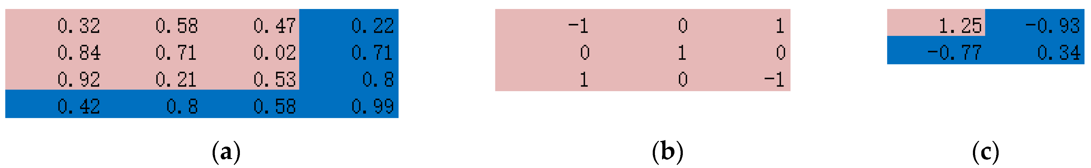Figure 1 displays an example of the convolution operation. A 3 × 3 filter is convolved through a 4 × 4 array and output a 2 × 2 array with values calculated by the dot product of the sliding filter and the original data value. If the input array has more than one channel, as in a natural image with RGB channels, there will be the 3rd dimension (depth) added to the previous two-dimension filer, and the output array will still be two-dimension with value summing over the depth dimensions. 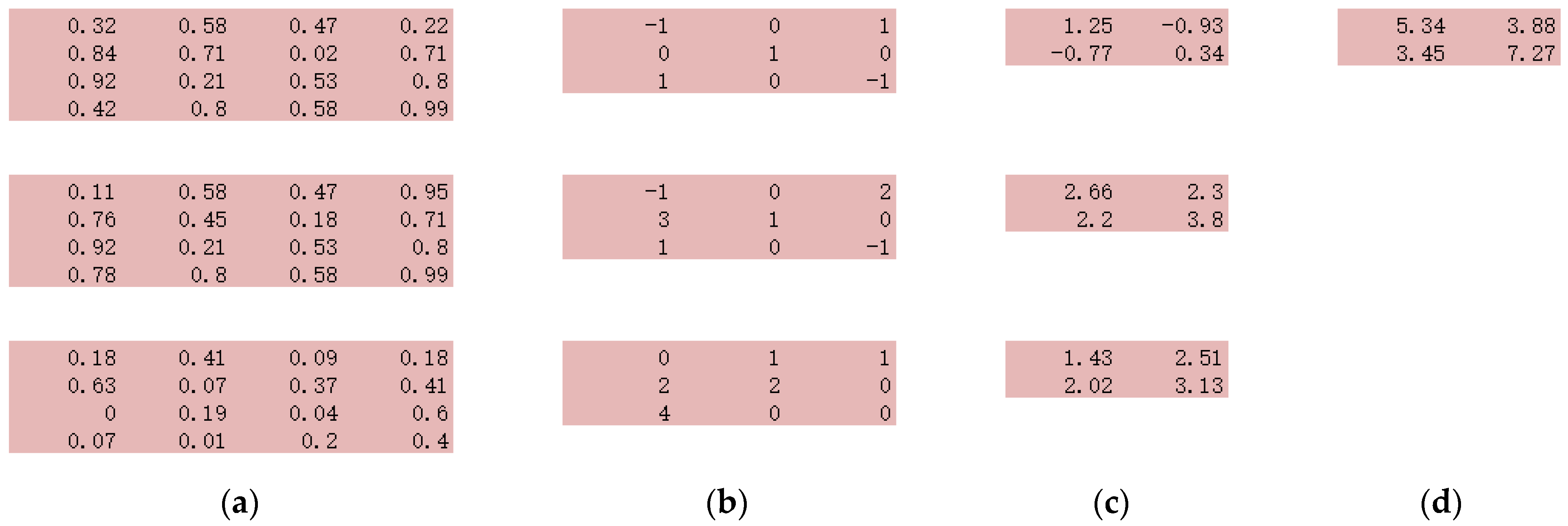Figure 2 shows a multi-channel example with a 4 × 4 image with three channels (Figure 2a). Three-dimension filters (Figure 2b) are designed, each one is applied to the corresponding channel, and the result will be 3 × 2 ×2 outputs (Figure 2c). Then these three outputs will be simply summed up together, leading to one 2 × 2 output (Figure 2d).

When the input is 3D arrays, the 3D filter, and its convolving operation are the same as that of 2D except that an additional dimension is added.

The above-described convolution procedure only extracts linear information, and for obtaining nonlinear information, an activation layer is introduced after each convolutional layer. Rectified Linear Units (ReLU) is the most commonly used activation function that maps negative values to 0, and keeps the positive values, respectively. This function will not affect the size of the data arrays and will be used in this work.

A pooling layer is usually applied after the convolution and activation transformation to reduce the input’s dimension in order to avoid overfitting, and unlike convolution, there is no overlap in pooling operations for each pooling layer. Max pooling is the most widely used pooling method, which selects the maximum value among all covered values as the output value.

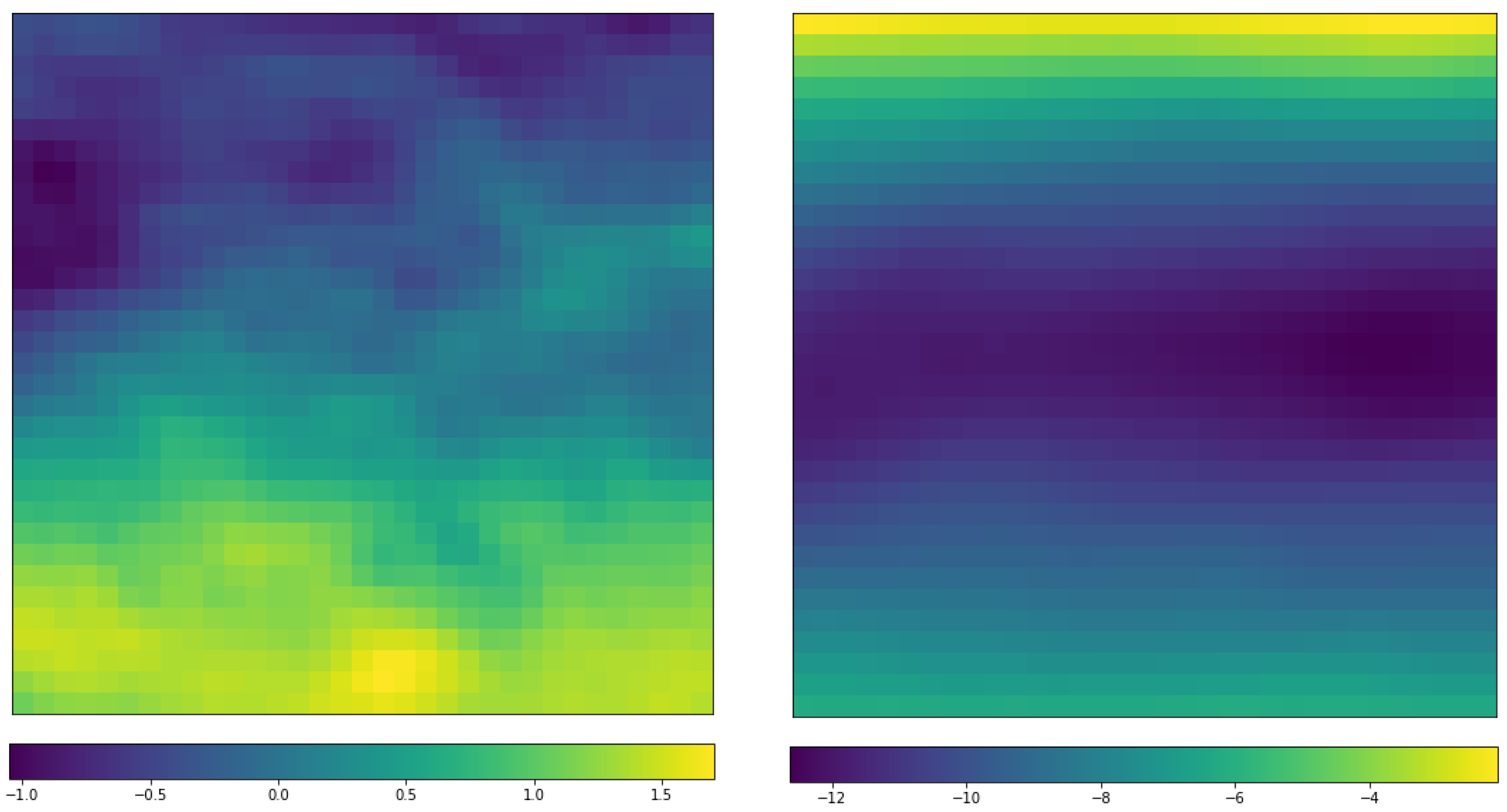
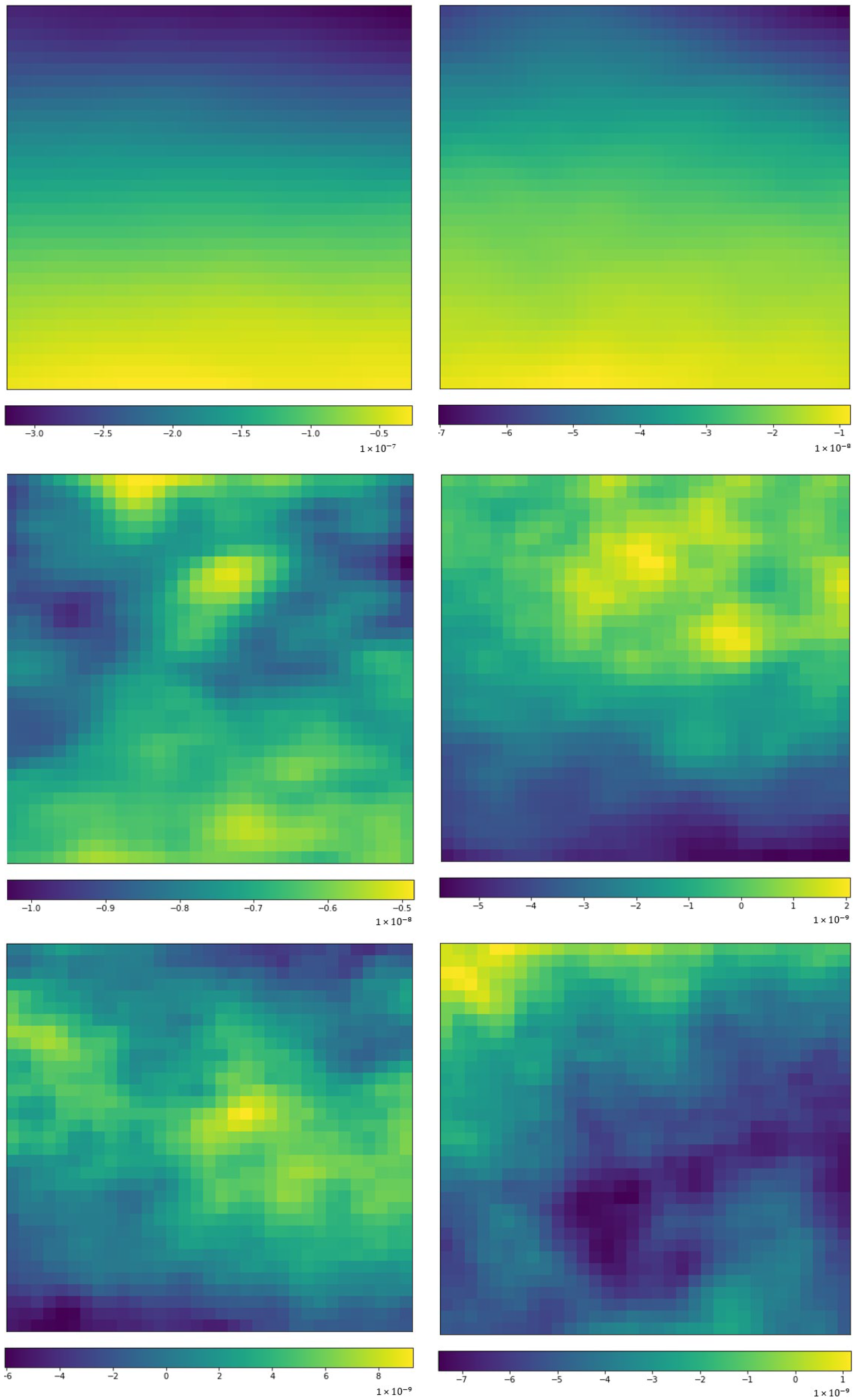
There are various types of deep learning models, and the most appropriate model for converting the gridded data into features for mining purposes is the auto-encoder network. Each auto-encoder network is composed of multiple deep learning layers, which is divided into two parts: an encoder represents a feature extraction process from the input and a decoder that reconstructs the input.

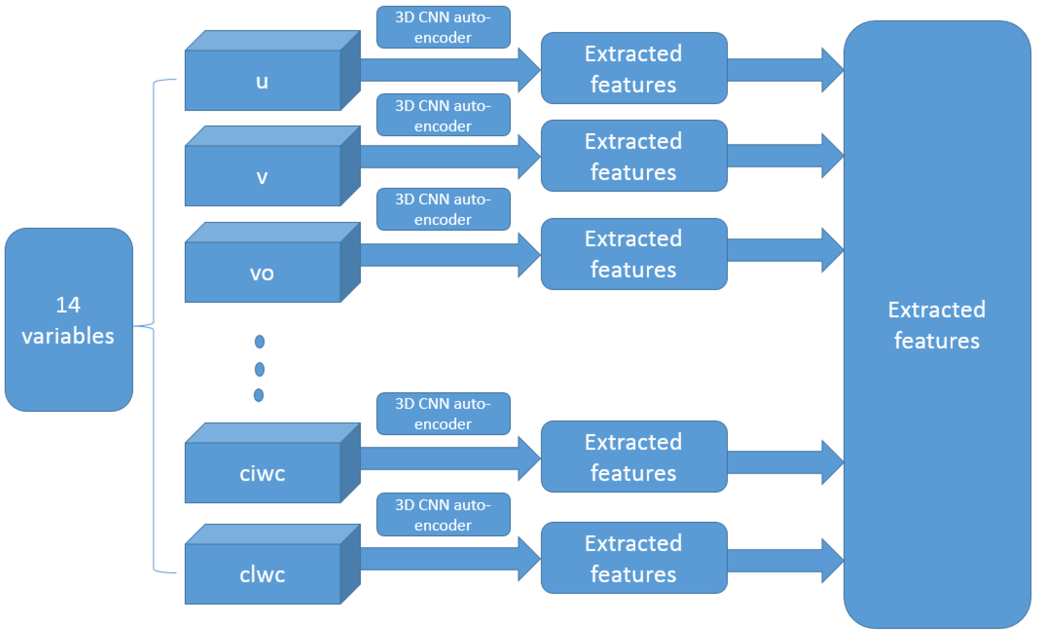
With the 14 × 4 × 37 × 33 × 33-dimensional ERA-Interim data, a more efficient auto-encoder network is a 3D Conv-auto-encoder. That is an auto-encoder with a group of 3D convolutional, activation (ReLU), and pooling layers. In each 3D convolutional layer, there are multiple 3D convolutional filters with learnable weights with an additional channel dimension on the input channels. Moreover, the 14 variables in ERA-Interim data are treated differently than the usual spatial or temporal dimension, and therefore, 14 different 3D Conv-auto-encoders are adopted to handle the ERA-Interim data.

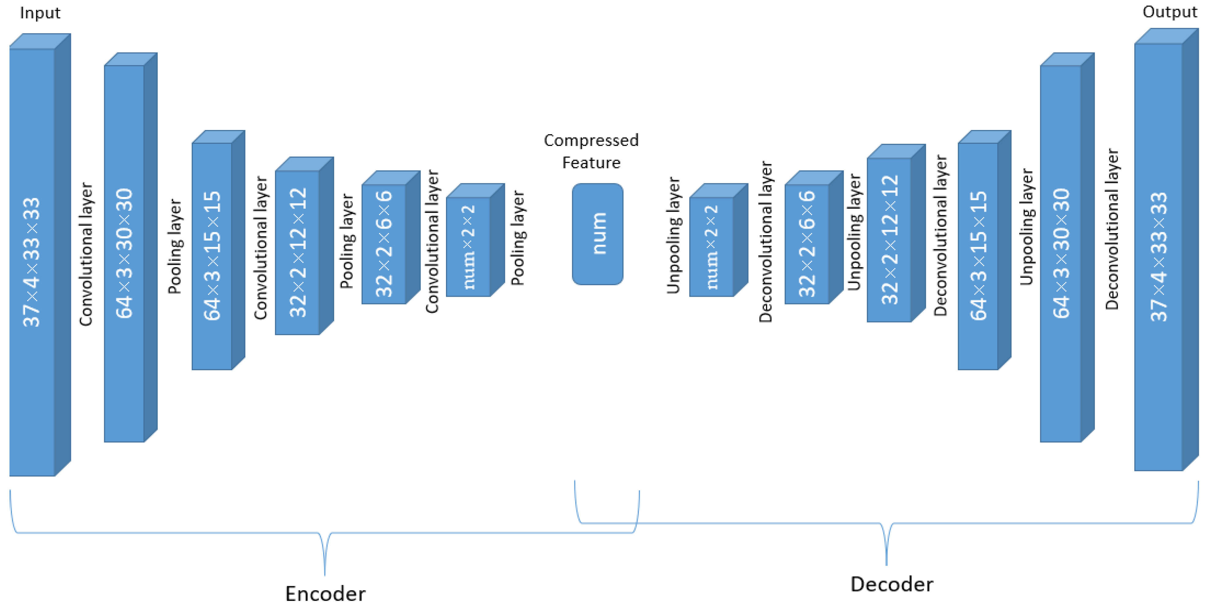
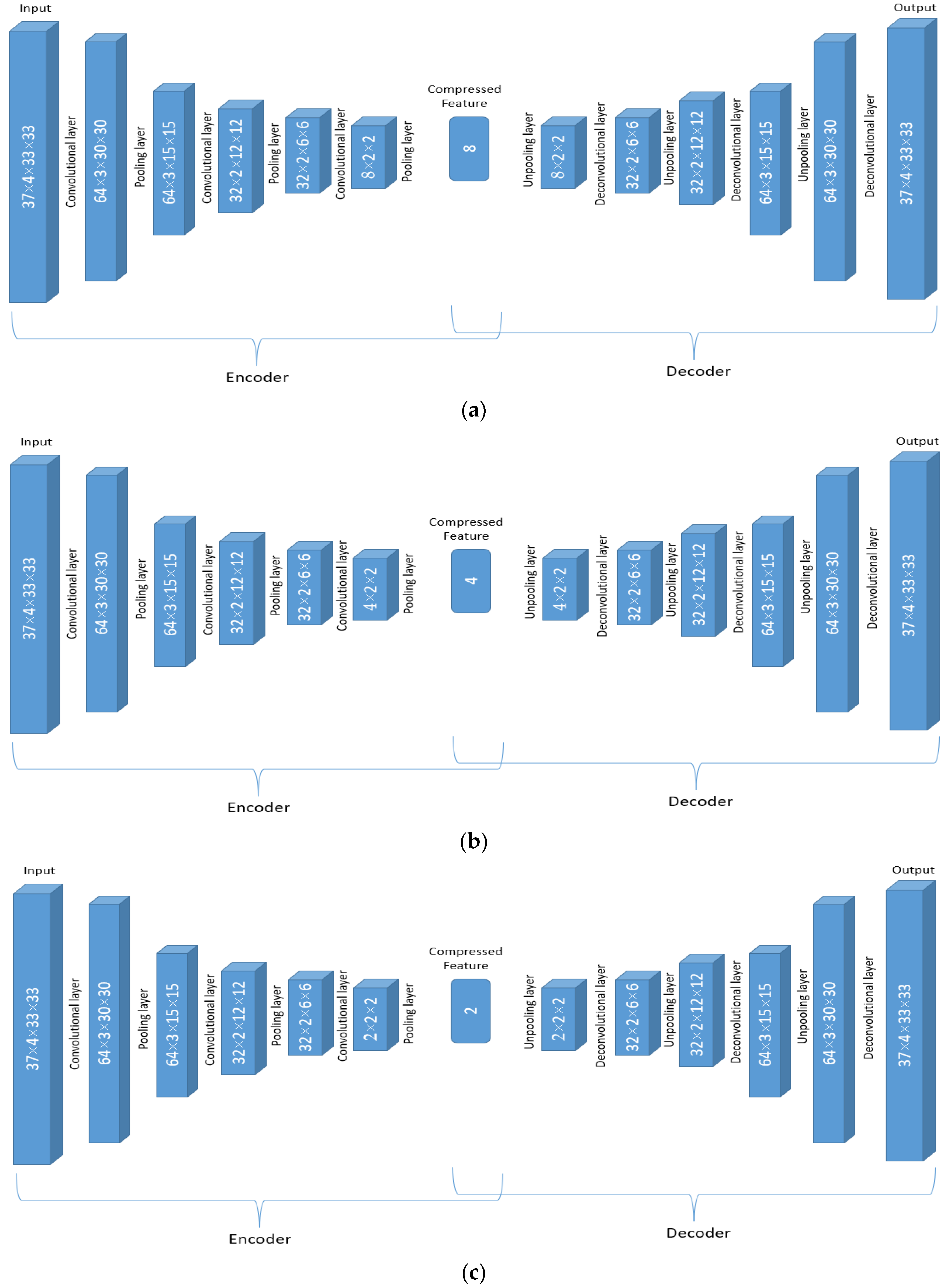
To be specific, the input of the encoder are observations with the dimension of 37 × 4 × 33 × 33, with pressure level (37) as its channel. There are 14 such auto-encoder networks. The network working on a single variable is elaborated below in detail, and the dimension changes in the data are displayed in Figure 3.

The first convolution layer is with 64 different 37 (channel) × 2 × 4 × 4 filters and converts the 37 × 4 × 33 × 33 array for one variable to 64 3 × 30 × 30 arrays. In other words, a 37 × 2 × 4 × 4 filter is applied, and the results are summed up in the channel dimension (37), and therefore the vertical pressure layer dimension number is reduced to 1. This procedure is repeated 64 times with different convolution weights. Therefore, after the first convolution layer, the original 37 × 4 × 33 × 33 array becomes 64 3 × 30 × 30 arrays. The activation applied after each filter in the convolution layer does not change the array size and therefore is not shown in Figure 3. After the convolution layer, A 1 × 2 × 2 pooling layer converts the 64 arrays with dimension 3 × 30 × 30 to 64 arrays with dimension 3 × 15 × 15.

The second convolution layer has 32 different filters with dimensions 64 × 2 × 4 × 4, and in this layer, the new dimension due to 64 different filters in the previous layer is considered to be “channels” and the filtered arrays will be summed over the channel dimension. As a result, each of the 32 filters converts the 64 × 3 × 15 × 15 array to 1 array with reduced dimensions 2 × 12 × 12 with the same operation as that of the first convolution layer, and finally, there are 32 such arrays. The same 1 × 2 × 2 pooling layer is then applied to the 32 2 × 12 × 12 arrays, and that results in 32 2 × 6 × 6 arrays. Similar to the previous two convolutional layers, the third convolution layer has num different convolution filters 32 × 2 × 5 × 5, and the dimension of 32 is treated as the channel again. The result after this filtering process is num arrays of dimension 1 × 2 × 2, where the num is a to-be-determined hyperparameter. Finally, the last 1 × 2 × 2 pooling layers will compress the arrays into num scalar features.

The decoder is the reverse of the encoder using the deconvolutional and unpooling layers in DeConvNet network [40,41,42] to reconstruct the convolutional networks, i.e., reverse the convolution and the pooling operations. More details about DeConvNet could be found in Zeiler et al. [40,41,42].

The network is trained through the backpropagation, where the mean square error [43] is used as the loss function, and Adam optimizer [44] is used as the optimizer to update the filter weights through backpropagation.

Fourteen separated networks with the same structure displayed in Figure 4 are trained separately for 14 different ERA-Interim variables. The compressed features from each of the networks are merged with filtered SHIPS variables and together used as the input of the GMM-SMOTE [27,28].

4. Results

4.1. Hyperparameters Tuning for the Autoencoder Structure

The framework of this study (TCNET) is almost the same as that for the LLE-SHIPS model, except that the ERA-Interim data are filtered with a CNN-based autoencoder network [28]. Unlike in the LLE-SHIPS model where all variables in the ERA-Interim data are treated together with only one dimension-reducing model for the feature extraction, one autoencoder network is trained to extract information from each of the 14 ERA-Interim variables. In other words, there are 14 different autoencoder networks in total for the 14 variables.

The to-be-determined hyperparameter, the dimension of the compressed feature (num) (see Figure 3), is preset as 8, and therefore, eight new variables are generated from each network, labeled as variable + order in the compressed feature layer (‘1’ to ‘8’). For example, v1 to v8 are new variables derived from the trained 3D CNN auto-encoder for variable v. The “num” is tuned in steps similar to the tuning process of SHIPS data filter [27].

First, train a separated 3D CNN auto-encoder for each of the 14 variables for 200 epochs. The training losses (mean square error) of 14 auto-encoder networks all converge after 100 epochs (not shown). Eight (num = 8) new variables are engineered from each ERA-interim variable first. Because of the characteristic of the auto-encoder, features with no information, i.e., zero feature, could be created, and those features are removed. A correlation check is conducted among the newly derived no-zero variables and against the 72 SHIPS variables [27], and highly correlated (r > 0.8) variables are also removed.

Second, the remaining output features of the ERA data filter (the auto-encoder with num = 8), and the output from SHIPS data filter (72 variables) [27] are concatenated together to form the input data set. Then the same Bayesian optimization (BO) with 40 iterations is used to tune hyperparameters for GMM-SMOTE and XGBoost together with no clustering and a preset 0.5 classification decision threshold [27,28]. Finally, the hyperparameter set with the highest 10-fold cross-validation is selected. Here, instead of kappa score used for COR-SHIPS and LLE-SHIPS, we use the importance score as a tuning criterion. The importance for each of the 14 variables is calculated as the sum of the importance scores of all components (up to 8) from the same variable. The final importance scores (IS), number of remaining features, and the specific removed features (for zero value and high correlation) are listed in

Table 1. The list of the 14 variables, their summed importance scores (IS), number of remaining features (Feature Number), and the specific removed variables due to all zero value and high correlation (bold font).

Variables	Name	IS	Feature Number	Removed Features
q	Specific humidity	0.065	5	q3, q8; q7
r	Relative humidity	0.064	7	r4
u	Horizontal wind	0.067	8
v	Meridional wind	0.062	7	v7
pv	Potential vorticity	0.056	6	pv7, pv8
vo	Relative vorticity	0.051	5	vo1, vo6, vo7
w	Vertical wind	0.043	5	w3, w4; w1
d	Divergence	0.042	3	d1, d4, d6; d2, d3
t	Temperature	0.024	4	t1, t2, t5, t6
z	Geopotential	0.020	3	z2, z3, z5, z7, z8
o3	mass mixing ratio	0.020	3	o31, o32, o33, o34, o36
clwc	Cloud liquid water content	0.013	2	clwc2, clwc4, clwc5, clwc6, clwc7, clwc8
cc	Fraction of cloud cover	0.017	1	cc2, cc4, cc5, cc6, cc7; cc3, cc8
ciwc	Cloud ice water content	0.011	1	ciwc2, ciwc3, ciwc4, ciwc5, ciwc6, ciwc7, ciwc8

.

As the summed importance score indicates how important the variable is, the more important variable (with a higher importance score) should be represented by more compressed features. Therefore, based on the summed importance scores, the 14 variables are categorized into three classes. If the IS is above 0.045, the dimension of the compressed feature (num) remains at 8. This is valid for variables q, r, u, v, pv, and vo and their corresponding auto-encoder is displayed in Figure 5a. If 0.02 < IS ≤ 0.045, num is set at 4. This is valid for variables, w, d, and t, and the corresponding auto-encoder structure is displayed in Figure 5b. For other variables with IS equal to or smaller than 0.02 (z, o3, cc, ciwc, and clwc), only two dimensions are selected (num = 2) as shown in Figure 5c.

After the new structures for DL Interim filters are derived, we retrain each network 200 times, although all the networks converge after 100 iterations. It should be emphasized that the randomness in the TCNET training process makes the training results different for different training sessions. However, the overall trends in the results should be similar if not the same. As same as being processed above, 19 variables, i.e., pv2, pv4, pv5, q1, u4, u7, v1, v2, vo2, vo7, w4, d1, d2, d4, t2, t3, t4, z1, and o32 are zero features, i.e., they contain all zeros, and are removed. cc2 is highly correlated (>0.8) with cc1, and w2 and w3 are highly correlated with w1. Hence cc2, w2, and w3 are removed. The remaining 48 (6 × 8 + 3 × 4 + 5 × 2 – 19 − 3) features are concatenated with the filtered SHIPS variables and are used as the input to the GMM-SMOTE.

4.2. Hyperparameters Tuning for GMM-SMOTE and XGBoost

After the hyperparameters in data filters are tuned, the hyperparameters for GMM-SMOTE and XGBoost still need to be tuned for the best results. The procedures are the same as those described in WY21 and WYK22 [27,28]. Therefore, without providing the tuning process, we report the values of the tuned parameters in

Table 2. Hyperparameters tuned for GMM-SMOTE and XGBoost. The Min and Max define the search ranges for each hyperparameter during the tuning processes. The initial value (before tuning, MB) and the final values (after tuning, MA) are given in the last two columns.

Hyperparameter	Component	Explanation	Min	Max	MB	MA
n_cluster	GMM-SMOTE	The maximum number of clusters in the Gaussian Mixture Model	1	10	1	3
m_neighbors	GMM-SMOTE	The number of nearest neighbors used to determine if a minority sample is in danger	3	10	10	10
k_neighbors	GMM-SMOTE	The number of nearest neighbors used to construct synthetic samples	3	14	5	9
shrinkage	XGBoost	Shrinkage ratio for each feature	0	0.3	0.1	0.19
n_estimator	XGBoost	The number of CART to grow	100	2000	100	2000
subsample	XGBoost	Subsample ratio of the training instances	0.5	1	1	0.5
colsample	XGBoost	Subsample ratio of columns for creating each classifier	0.5	1	1	1
reg_alpha	XGBoost	L1 regularization term on weights	0	20	0	0.5
reg_lambda	XGBoost	L2 regularization term on weights	0.5	20	1	20
gamma	XGBoost	Minimum loss reduction required to make a further partition on a leaf node of the CART	0	10	0	0
min_child_weight	XGBoost	Minimum sum of instance weight in a split	0.5	5	1	0.5
max_depth	XGBoost	Max depth of each CART model in XGBoost	3	10	3	3
decision threshold	XGBoost	Decision threshold on the XGBoost classifier output	0	1	0.5	0.2

. Readers interested in the details are referred to [13].

4.3. Model Results on Test Data

Similar to LLE-SHIPS model, the evaluation of the prediction for the TCNET model is on the test data only. The test confusion matrix for the model, before hyperparameter tuning (MB), and after hyperparameter tuning (MA) is displayed in

Table 3. Confusion matrix values after (before) hyperparameter tuning with the test data. The RI definition is the original definition by Kaplan and DeMaria (30 kt/day Vmax increase) [5].

	Predicted RI	Predicted Non-RI	Actual
Actual RI	48 (29)	47 (66)	95
Actual non-RI	37 (31)	1465 (1471)	1502
Total Predicted	85 (60)	1512 (1537)

. The increase of correctly predicted RI cases indicates that the hyperparameter tuning procedure does help the model performance.

Kappa, PSS (Peirce’s skill score), POD, and FAR are used here for the model evaluation, and their values for MB and MA are elaborated in

Table 4. Performance comparisons for the tuning benefit. MB and MA denote the models before and after the hyperparameters in GMM-SMOTE and XGBoost are tuned.

Model	Kappa	PSS	POD	FAR
MB	0.344	0.285	0.305	0.517
MA	0.506	0.481	0.505	0.435
Improvement	47.10%	68.80%	65.60%	−15.90%

. After tuning, POD increases 65.6% from 0.305 to 0.505, while FAR decreases from 0.517 to 0.435 (15.9%). The overall statistics PSS and Kappa score also increased from 0.285 to 0.481 (68.8%) and from 0.344 to 0.506 (47.1%), respectively, confirming the substantial improvement in RI prediction with the hyperparameter tuning procedure. Apparently, the model was overfitted before the tuning process with so many variables.

4.4. Performance Comparison

As in WYK22 [28], we aim to compare the performance of the TCNET model against the baseline COR-SHIPS first.

Table 5. Performance metric values for the COR-SHIPS, LLE-SHIPS, TCNET, Y16 and KRD15 models and the comparisons of TCNET model developed in this study vs. the baseline model, COR-SHIPS, Y16 and KRD15 represented by the improvement.

Model	Kappa	PSS	POD	FAR
COR-SHIPS	0.354	0.368	0.411	0.621
LLE-SHIPS	0.454	0.399	0.421	0.563
TCNET	0.506	0.481	0.505	0.435
Y16	0.275	NA	0.34	0.711
KRD15	NA	0.225	0.275	0.825
vs. COR-SHIPS	42.9%	30.7%	22.9%	−30.0%
vs. Y16	84.0%	NA	48.5%	−38.8%
vs. KRD15	NA	114.0%	83.6%	−47.3%

shows the values of Kappa, PSS, POD, and FAR for both models, with the values for the LLE-SHIPS model [28] as references. TCNET performs better than LLE-SHIPS, and the improvement over the baseline COR-SHIPS is substantial with 42.9%, 30.7%, 22.9%, and 30.0% in terms of kappa, PSS, POD, and FAR, respectively. It is worth noting that the 48 newly derived features in the TCNET model are almost half of the 90 variables generated by LLE [28], and this fact shows that using large-scale ERA variables provides much more information than incorporating near core ERA variables only in RI prediction. Of course, here, the structure of the data is partially preserved with the CNN framework but for the LLE process, the values in near center areas are averaged.

Two other works, i.e., the best results in RI prediction research by Yang [45] (hereafter, Y16) and Kaplan et al. [6] (hereafter, KRD15), which outperform almost all of the other works, are used to compare with the performance the newly developed RI prediction model, too. The corresponding valid values for the four performance measures are also listed in Table 5. The POD improvement is 48.5% and 83.6% over Y16 and KRD15, respectively while the FAR were reduced by 38.8% and 47.3%. Please note the ERA-Interim data are retrospectively generated with comprehensive data sources “after the fact”. Therefore, the model cannot be directly used for forecasting purposes, and it is not fair to compare with operational RI prediction models, which give much lower POD with comparable FAR (table 6 in [7]). Even with that limitation, the results here, in particular the newly identified RI impacting features, should shed a light on understanding of RI and potentially help the improvement of the statistical-dynamical-based RI predictions.

4.5. Feature Importance

Similar to the LLE-SHIPS model, the importance scores could be derived from XGBoost for the output of the data filters. However, in the TCNET model, since there are even significantly more variables (each grid in each variable could be regarded as a feature) than that of the input for the LLE data filter, it is even more computationally expensive and impossible to implement the same feature importance evaluation approach (permutation) as in LLE-SHIPS model. In other words, tracing back the importance of each ERA-Interim feature is almost impossible for the TCNET model. Therefore, although we can evaluate the importance of the output of data filters, how to evaluate the contribution from each of the original ERA-Interim variables is a notoriously difficult task for deep learning networks, a.k.a, the autoencoder network. Here we roughly evaluate the importance of the ERA-Interim variables by calculating their summed importance score derived from the XGBoost classifier for each of the 14 ERA-Interim variables, as well as the averaged individual score for parameters associated with each variable. In addition, for variables with a higher importance score, feature level information from the individual 3D auto-encoder is traced back based on the feature map [42], where the extracted information, for example, the geometric location, is visualized, and the maps of selected variables.

Table 6. The variables with top 10 importance scores (IS) in the TCNET model and their description.

Variable	IS	Description
BD12	0.019747	The past 12-h intensity change
VMAX	0.0176	Maximum Surface Wind
SHRD	0.01481	850–200 hPa shear magnitude
DTL	0.014381	The distance to nearest major land
IRM1_5	0.013737	Predictors from GOES data (not time dependent) for r = 100–300 km but at 1.5 h before initial time
o31	0.013308	1st variable in o3
G150	0.013093	Temperature perturbation at 150 hPa due to the symmetric vortex calculated from the gradient thermal wind. Averaged from r = 200 to 800 km centered on input lat/lon (not always the model/analysis vortex position)
q7	0.013093	7th variable in q
u3	0.012878	3rd variable in u
q4	0.012878	4th variable in q

displays the 10 most important variables among the 120 selected variables including 72 SHIPS variables, and the 48 variables extracted from the DL ERA-interim data filter. The importance scores of all the 120 variables are given in

Table A1. The importance scores of all of the 120 variables.

IS	Variable	Ranking	IS	Variable	Ranking	IS	Variable	Ranking
0.02	BD12	1	0.009	vo6	41	0.007	Z850	81
0.018	VMAX	2	0.009	MTPW_1	42	0.007	SHTD	82
0.015	SHRD	3	0.009	u2	43	0.007	NOHC	83
0.014	DTL	4	0.009	r4	44	0.007	OAGE	84
0.014	IRM1_5	5	0.009	pv7	45	0.006	XD18	85
0.013	o31	6	0.009	pv6	46	0.006	IR00_3	86
0.013	G150	7	0.009	PSLV_1	47	0.006	IRM1_16	87
0.013	q7	8	0.009	TADV	48	0.006	PSLV_4	88
0.013	u3	9	0.009	v8	49	0.006	NTFR	89
0.013	q4	10	0.009	HIST_2	50	0.006	HIST_9	90
0.013	G200	11	0.009	VMPI	51	0.006	ND20	91
0.013	vo3	12	0.009	V300	52	0.006	IR00_14	92
0.012	REFC	13	0.009	SHRS	53	0.006	IRM3_17	93
0.012	vo5	14	0.009	VVAC	54	0.006	EPSS	94
0.012	vo8	15	0.009	MTPW_19	55	0.006	clwc2	95
0.012	PEFC	16	0.009	v5	56	0.006	D200	96
0.012	d3	17	0.008	t1	57	0.006	V850	97
0.012	CFLX	18	0.008	RD26	58	0.006	PC00	98
0.012	PSLV_3	19	0.008	SDDC	59	0.006	r8	99
0.011	T150	20	0.008	q6	60	0.005	u5	100
0.011	jd	21	0.008	O500	61	0.005	NDFR	101
0.011	R000	22	0.008	v7	62	0.005	PCM1	102
0.011	TWXC	23	0.008	IRM3_11	63	0.005	NSST	103
0.011	u8	24	0.008	E000	64	0.005	PENV	104
0.011	PW08	25	0.008	PW14	65	0.005	TGRD	105
0.011	q3	26	0.008	z2	66	0.005	IRM3_14	106
0.011	XDTX	27	0.008	G250	67	0.005	IR00_20	107
0.011	CD26	28	0.008	pv1	68	0.005	T250	108
0.011	q8	29	0.008	cc1	69	0.005	RHMD	109
0.011	pv3	30	0.008	XDML	70	0.005	IRM1_14	110
0.011	v4	31	0.008	pv8	71	0.005	IRM1_17	111
0.011	r1	32	0.007	vo1	72	0.005	cc2	112
0.01	u1	33	0.007	ciwc1	73	0.003	NDTX	113
0.01	q5	34	0.007	v3	74	0.003	r7	114
0.01	IR00_12	35	0.007	SHTS	75	0.003	TLAT	115
0.01	vo4	36	0.007	v6	76	0.002	PCM3	116
0.01	HE07	37	0.007	ciwc2	77	0.002	HIST_16	117
0.01	u6	38	0.007	w1	78	0.0006	r2	118
0.01	q2	39	0.007	IRM3_19	79	0	r3	119
0.009	r6	40	0.007	IR00_17	80	0	r5	120

. We can find that among the top 10, there are six SHIPS variables and four DL variables. The importance score (IS) is scaled in such a way that the sum of all IS values is equal to one. We found that the total importance score for the 48 DL variables is 0.4119 and for the SHIPS variables, 0.5881. Therefore, the average score per SHIPS [ERA] variable is 0.0082 [0.0086]. The fact that the average score for the SHIPS variable is less than that of ERA variables indicates that the ERA-Interim data filter has a similar importance score compared to that of SHIPS variables; hence DL ERA-interim data filter is working efficiently.

Since the 3D auto-encoder model structure is different over 14 ERA-Interim variables, the summed importance scores as well as the average score per valid feature should be considered.

Table 7. Summed variable importance score and its ranking, the number of non-zero, non-correlated features, the feature-wise averaged importance score, and its ranking for each ERA-Interim variable.

Variables	Summed IS	Feature Number	IS Rank	Average IS	Average IS Rank
q	0.0759	7	1	0.0108	3
vo	0.0635	6	2	0.0106	4
u	0.0585	6	3	0.0098	5
v	0.0509	6	4	0.0085	7
pv	0.0441	5	5	0.0088	6
r	0.0387	8	6	0.0048	14
ciwc	0.0144	2	7	0.0072	10
o3	0.0133	1	8	0.0133	1
cc	0.0120	2	9	0.0060	12
d	0.0118	1	10	0.0118	2
t	0.0082	1	11	0.0082	8
z	0.0077	1	12	0.0077	9
w	0.0071	1	13	0.0071	11
clwc	0.0058	1	14	0.0058	13

displays the total scores and the average scores per feature for all the 14 variables. The specific humidity (q), relative vorticity (vo), and zonal component of wind (u) are scored in the top 5 in terms of both summed score and the average score.

The famous problem with DL is difficulties in the interpretation of the results. Here we try to shed lights on the learning process and the result explanation with more displays. The first group of displays consist of the feature maps showing the value distributions after the first layer in the auto-encoder network (referred to Figure 5).

Figure 6 shows the feature maps after the first convolutional layer of the network for variable q, the relative humidity, with the demonstrated structure in Figure 5a. The 64 × 3 × 30 × 30 information are presented in 64 × 3 30 × 30 maps, i.e., each tiny map is with 30 × 30 pixels, and 64 of them are grouped in one panel, and there are three such panels after the first convolutional layer. The maps conserve the relative locations after the original values are convoluted with local filters. However, the order in other dimensions is broken down but the corresponding positions are preserved with different instances through the same network.

From this figure, we find that the extracted feature maps are quite sparse with many empty maps. Careful checking of those maps reveals that there are roughly 22 to 24 non-empty feature maps in each 64-feature-map group. One apparent difference between the RI and non-RI instances is that the trained filter catches more information (more colored areas) in the non-RI case than that in the RI case. This possibly indicates that the q fields in non-RI cases are relatively more uniform than the corresponding fields of RI cases. Another observation is that most selected features for the RI instance concentrate in the southeast of the center (bottom right). Therefore, we can conclude that the specific humidity (q) in southeast of the center is more important in RI occurrence.

Another feature map group is displayed in Figure 7 for zonal component of wind (variable u). in this case, the non-zero feature maps are even fewer, only 11/64 non-empty features identified for both the non-RI and RI instances. For this variable, the major character of those displays is that features are mainly retrieved with north-south structures. The feature maps for relative vorticity (vo) are also checked (not shown). Only seven non-zero features are identified, and the features are of vertical structures across the north and south ends as well as the middle parts.

Although the feature maps demonstrated the feature retrieval procedure, they could not give much help on defining practical RI-related features based on the selected parameter (for q or u or any other variables). For this purpose, we need to go back to the physical variables and show the behaviors of RI instances and non-RI ones and compare the differences between them.

Figure 8 shows the distribution of average q for RI instances and non-RI instances. One can see that the high values are mainly concentrated in the southeastern corner as identified by the corresponding feature maps. As expected, in RI cases, the mean humidity is generally higher than that for the non-RI cases. However, the difference is not uniformly distributed around the TC centers. The differences between them are displayed in Figure 9. In SHIPS database, the humidity related parameters are those defined with relative humidity from 300 to 1000 hPa (RHHI, RHMD, RHLO, and R000), and most of time, RHLO is singled out for its deterministic impact on RI [5]. The displays in Figure 9 support the conclusions. However, SHIPS uses average values in 200–800 km circular bands around TC centers. The results displayed in Figure 9 demonstrated the differences between RI and non-RI averaged humidity is not uniformly distributed. In 1000 (not shown) to 700 hPa, the differences are the highest east of the TC centers but around the middle in the meridional direction. The difference is close to uniform at 500 hPa but becomes more concentrated at 300 hPa around the middle in the vertical direction but almost across all longitudes.

The selected displays of the distribution of the second important parameter vo, relative vorticity, are displayed in Figure 10. First, with the corresponding parameter in SHIPS database, the averaged 850 hPa vorticity in r = 0–1000 km area (Z850), we displayed the distribution of mean differences of relative vorticity between RI and non-RI samples at 850 hPa. It seems that it is hard to say the roles of this parameter at this level in the RI cases because the values are kind of randomly varying between positive and negative values. However, when we raise the level to 300 hPa, the difference field shows a clear pattern, positive differences in the south of the TC centers and negative differences far away from the centers in the north direction. The mean fields of the RI instances and non-RI instances obviously support the difference, although all relative vorticity values in this level are negative. The transition from lower random pattern to the organized pattern in higher layers takes place around 500 hPa.

The third important parameter identified via the TCNET is the u-component of the wind, and the selected distributions are demonstrated in Figure 11 and Figure 12 The field images in Figure 11 show that the overall patterns are similar for RI and non-RI means at 850 and 200 hPa although the details are different. The high wind is relatively concentrated in RI cases but more scattered in the non-RI cases at both 850 and 200 hPa levels. Actually, from the distribution, one can derive the commonly accepted conclusion that the vertical shear of the horizontal wind between 850 and 200 hPa levels is weaker in RI cases when compared with that of the non-RI cases. The wind difference between RI and non-RI cases is shown in Figure 12. At 850 hPa, the positive difference in the lower part may be simply interpreted by stronger TCs in general during RI, and the negative values at 200 hPa are related to stronger wind shear in the non-RI cases.

Figure 13 shows the differences of ozone mass mixing ratio (o3) between the RI cases and non-RI cases. Ozone concentration is highest between 10 to 20 km above the surface or around 200 to 50 hPa [46]. A strong upper tropospheric downward motion would make high ozone on top of TCs [47]. It is clear to see that the ozone difference is all negative in high layers (at 100, 200, and 300 hPa). This can be explained by the fact that RI TCs are usually higher in the vertical structure than those non-RI cases. This is not a surprise because a taller structure means more ventilation and more energy to the TCs. As we move the observations downward, we find that the difference is of mixed positive and negative values at 500 and 800 hPa, and the horizontal pattern is not evident. At the surface (1000 hPa), most of the differences are negative values with a little positive difference in the north-western corner. However, due to the relative smaller ozone values in lower layers, it is hard to say much about how the ozone impacts to the RI processes.

5. Conclusions and Discussion

To enhance RI prediction with modern machine learning techniques, we extended a well-tailored artificial intelligence (AI) system [27]. This system consists of four major components, data filters to remove variables unrelated to RI, reduce variables among highly correlated variables, screen out variables with high missing value rates, and engineer/extract a reduced set of variables from the high-dimensional variable space; a customized sampler to upsample the minority (RI) instances and downsample majority instances simultaneously by a GMM-SMOTE sampler; a very powerful state-of-the-art classifier, the XGBoost, to classify instances into RI and non-RI and to evaluate variable importance based on the information gain; a hyperparameter tuning procedure tweaking hyperparameters appearing in all of the three above components, within pre-defined value ranges.

The first implementation of the system is for COR-SHIPS, a model depending only on SHIPS data as a new ML-based RI prediction system as well as a baseline for other ML-enhanced RI predictions [27]. One step further, the ECMWF ERA-Interim reanalysis data were also included in this framework in the hope to derive RI impact features beyond SHIPS. A model based on local linear embedding (LLE) for feature extraction from data near TC centers (small scale), the LLE-SHIPS model, was created and the RI prediction power was improved with the introduction of new data [28].

In this study, we extended the DL framework further to use a CNN-based auto-encoder network (TCNET) to derive features from the large-scale environment around TCs within the ECMWF ERA-Interim reanalysis data. The so-called TCNET model was discussed in detail in terms of the learning structure and learning processes and results, and its performance in RI prediction was compared with the COR-SHIPS and LLE-SHIPS models. We used the same training/validation data splitting and reported the performance based on the validation/testing data only. Three models are selected for the comparisons, KRD15, Y16, and COR-SHIPS, and the most commonly used metrics, kappa, PSS, POD, and FAR are evaluated.

It was found that the TCNET model outperforms Y16 and COR-SHIPS by 84% and 43% in kappa, and KRD15 and COR-SHIPS by 114% and 31% in PSS. On the positive POD, the current model improved the three reference models, KRD15, Y16, and COR-SHIPS by 83.6%, 48.5%, and 22.9%, respectively. In the meantime, the negative FAR is reduced by 47.3%, 38.8%, and 30.0%, respectively.

Although the three models based on the ML framework, COR-SHIPS, LLE-SHIPS, and this TCNET, all substantially improve the prediction of RI compared with traditional statistical models (KRD15 and Y16), understanding the mechanism for the performance improvement is not easy because of the famous black-box issue with ML, deep learning. For that purpose, we investigated the relative importance scores among the original SHIPS variables and the corresponding variables in reanalysis data sets. Most of the findings with the gridded reanalysis data sets are consistent with those identified within SHIPS databases. Moreover, the detailed investigation guided by the learning results reveals that the impacts of certain variables on RI depend on not only the averages of the values but also the orientation of value distributions. For example, at 850 to 700 hPa, the differences between RI and non-RI specific humidity averages show the highest values east or northeast of the TC centers (refer to Figure 9). For the relative vorticity (vo), the RI/non-RI difference field at 300 hPa shows a clear pattern, positive differences in the south of the TC centers and negative differences far away from the centers in the north direction (Figure 10). The horizontal wind (u) also shows a clear south-north difference pattern instead of a pattern of circular shapes.

An interesting variable we discovered but was not included in SHIPS databases is the ozone mass mixing ratio (o3). The impact of ozone on RI may not be strong for most TCs except for those tall TCs because the difference fields below 300 hPa show complicated patterns. Therefore, in most composite analyses, usually on data below 200 hPa, it may be difficult to find any obviously distinguishable patterns between RI and non-RI cases. Ozone has been related to TC development for quite some time and was introduced in the TC simulations [48,49]. Ozone is closely related to potential vorticity (PV) in middle and high latitudes and reflects the top structure of TCs [47]. Here, we tried to attribute the ozone role in RI to its relationship to the height of TCs, consistent with [47].

This model (TCNET) as well as the other two models based on the same framework, COR-SHIPS and LLE-SHIPS, significantly improve the RI prediction based on traditional performance measures. However, the reanalysis is not available for real-time forecasting unless the general prediction models can provide the same quality of data for the future at the predicting time. At this moment, we intend to use the after-fact reanalysis data for helping us to understand the RI mechanism or to identify new impact factors.

In all the three models under this framework, the “negative” time is limited up to 18 h before RI onsets based on the selections of previous statistical analyses and models. Earlier warning on potential RI scenarios could be helpful for operational forecasting (we thank one anonymous reviewer for pointing this out). Therefore, extending the before RI time beyond −18 h could be helpful with TCNET because not much computing is involved in the ML procedure. In that way, the RI will not only be forecasted at onset but also warned some time before the onset. Of course, in those cases, the parameter investigation such as those via Figure 8, Figure 9, Figure 10, Figure 11, Figure 12 and Figure 13 should include the distribution of parameter values before the current time.

As for the ML part, one potential implementable improvement is to define convolution filters based on the TC shape, or filters with the circular, sectorial, and annulus shapes with variable radii and sectorial angles, which may be more effective and efficient for TCs. The difficult part is to uncover what is going on inside the DL black boxes, which seems almost impossible.