A Method for Assessing Background Concentrations near Sources of Strong CO₂ Emissions

Abstract

In the quantification model of emission intensity of emission sources, the estimation of the background concentration of greenhouse gases near an emission source is an important problem. The traditional method of estimating the background concentration of greenhouse gases through statistical information often results in a certain deviation. In order to solve this problem, we propose an adaptive estimation method of CO₂ background concentrations near emission sources in this work, which takes full advantage of robust local regression and a Gaussian mixture model to achieve accurate estimations of greenhouse gas background concentrations. It is proved by experiments that when the measurement error is 0.2 ppm, the background concentration estimation error is only 0.08 mg/m³, and even when the measurement error is 1.2 ppm, the background concentration estimation error is less than 0.4 mg/m³. The CO₂ concentration measurement data all show a good background concentration assessment effect, and the accuracy of top-down carbon emission quantification based on actual measurements should be effectively improved in the future.

1. Introduction

As CO₂ emissions from strong point sources account for more than 33% of all anthropogenic emissions [1], monitoring the emission rates of strong point sources is essential for evaluating climate change and energy use efficiency [2]. Currently, the estimation of strong sources mainly refers to inventories, which help us assess the general CO₂ emission characteristics of national scale [3]. However, emission inventories are updated slowly and with low accuracy [4]. Moreover, no self-reported emission inventories are publicly available in some developing countries. “Top-down” assessment based on real-time monitoring of greenhouse warming gas concentration data will provide us with fast and accurately reported CO₂ emissions data, which will help with the formulation of emission reduction policies [5].

With the development of measurement technologies for greenhouse warming gases, multiple measurement systems can rapidly target the distribution of greenhouse gas concentrations in the vicinity of emission sources with high spatial and temporal resolution [6,7,8]. High-precision and near-real-time assessment of the emission rate can be achieved by dispersion models [9,10,11]. In situ measurements based on mobile systems can collect surface greenhouse warming gas data around emission sources, and through the Gaussian dispersion model, the emission position and rate can be determined [12]. Vehicle-based different absorption LIDAR (DIAL) can measure the CO₂ profile concentration based on the Mies scattering of aerosols [13]. This can provide a large amount of CO₂ concentration data, which are beneficial for reassessing the dispersion characteristics of the emission source [14]. However, the construction of a DIAL system is complex and costly, which may not be acceptable in most application scenarios [15,16]. The Unmanned Aerial Vehicle-based AirCore system determines methane emissions from mine ventilation shafts by collecting concentrations in downwind cross-sections based on a Gaussian diffusion model or mass balance method [17,18]. Airborne-based spectrometers covering the short-wave infrared (SWIR) spectrum can retrieve gas emission data from multiple strong emission sources in regions by measuring the column concentrations of CO₂ and NOx gases [19,20]. The Orbiting Carbon Observatory-2 (OCO-2) monitors the distribution of CO₂ air dry concentration (XCO₂) globally. Its spatial resolution is 2.25 km × 1.29 km [21,22,23]. OCO-3 can also monitor the distribution of CO₂ air dry concentration (XCO₂) globally [24]. They can be used to evaluate CO₂ emissions from power plants based on the enhanced concentration modeled by a two-dimensional Gaussian diffusion model [25,26].

It should be noted that all “top-down” assessments define the background concentration of gases. The background concentration will determine the value of the enhanced concentration caused by the emission source, which will further cause an incorrect estimation of the emission rate [27]. Most background concentration determination methods are based on statistical methods. Nassar determined the background value by averaging sections of the OCO-2 swath in one of two directions from the plume. As the choice of region was somewhat subjective, Nassar determined the background uncertainty by selecting four different plausible background regions and taking the standard deviation of the emission estimates from this ensemble of different backgrounds [25]. In Andersen’s study, the background concentration of methane was regarded as the sampled concentration that was not affected by the plume, which refers to the minimum value of the gas collections [18]. Due to the AirCore only collecting gas concentrations on a small scale, it is very likely that the methane background would be overestimated. Pei proposed calculating the background concentration of a city’s emissions using the Lagrangian approach [27] and demonstrated this method by overpassing OCO-2 over Riyadh. However, the technical requirements of the Lagrangian approach are difficult for users to apply in a wide range of scenarios. Therefore, there is an urgent need to develop a practical, stable, and accurate background concentration determination method to further improve the accuracy of carbon emission assessment.

In the remaining parts of this work, we introduce the basic principles for rapidly extracting the background concentrations of greenhouse gases near strong emission sources in Section 2 and then introduce the basic principles of the Gaussian plume model in Section 3. Based on the model, the gas concentration is simulated. By retrieving the simulated values, the accuracy of our algorithm evaluated. At the same time, the background concentration of greenhouse gases is estimated via OCO-2 satellite XCO₂ observations and mobile equipment CO₂ concentration measurements to verify the algorithm’s performance on different measurement data. Finally, we discuss the impacts of different clustering algorithms on the estimation of GHG background concentrations.

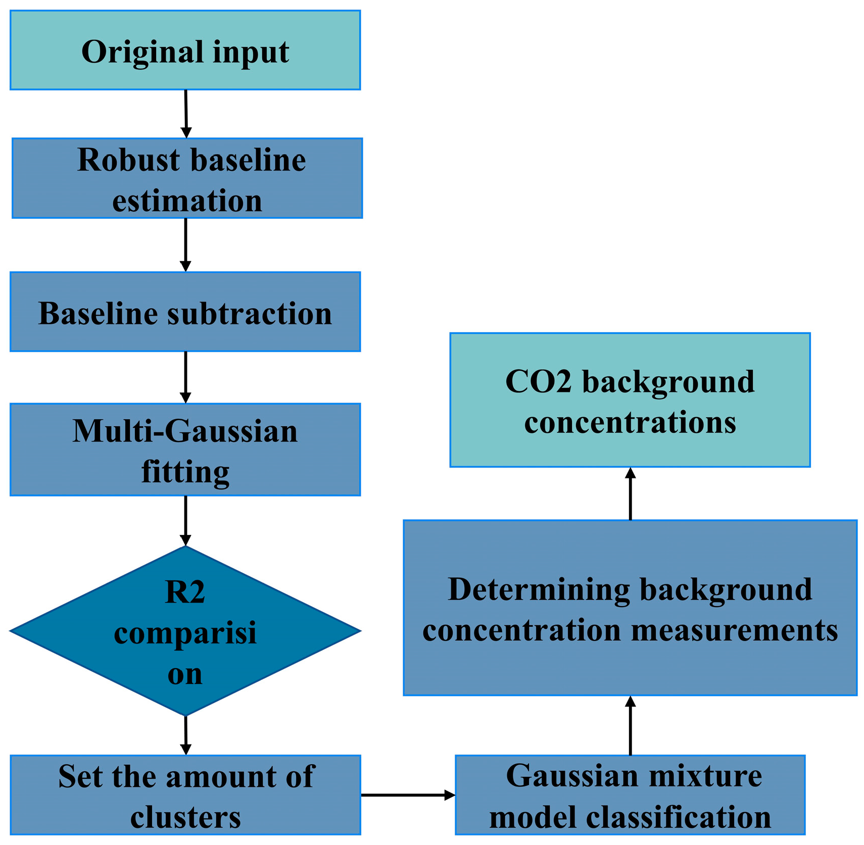
2. Methods

In this work, we divide the CO₂ concentration measurements into two parts, one for background concentrations that are less influenced by the source of strong CO₂ emissions and the other for enhanced CO₂ concentrations that are more influenced by the source of strong CO₂ emissions. In order to estimate the background concentration near the source of strong CO₂ emissions, we first roughly estimate the background concentration by means of robust local regression [28]. We then perform multivariate Gaussian fitting on the measurements subtracted from the roughly estimated background concentration to determine the number of peaks present in the measurements. Finally, we use the number of peaks, adding one as the number of Gaussian mixed model (GMM) clusters, and identify the measurements belonging to the background concentration. By averaging these measurements, we can obtain the background concentration near the source of strong CO₂ emissions. The steps are shown in the Figure 1.

2.1. Robust Local Regression

Obtaining the baseline in a signal through robust local regression is a common method that has been used for a long time, especially in relation to spectral signals. Compared with global regression, robust local regression reduces interference outside the background signal, making the final estimated background signal closer to the true background signal. In this study, we consider the CO₂ background concentration to be the baseline in the CO₂ concentration measurements, meaning we can express the CO₂ concentration measurements as in Equation (1), where $Y\left(x_i\right)$ is the observed CO₂ concentration at $x_i$, $b\left(x_i\right)$ is the background concentration, $s\left(x_i\right)$ is the CO₂ concentration enhancement due to the CO₂ emissions, and $e_i$ is the instrument measurement error. Under the basic assumption of robust local regression, $b\left(x\right)$ is sufficiently smoothing so that we can express it as a polynomial pair, $b\left(x\right)=b\left(x;\theta \right)$. Under this basic assumption, we can obtain the optimal estimate $\widehat{\theta }\left(x\right)$ at each point $x$ so as to obtain an estimate $b\left(x\right)$ by minimizing the loss function (Equation (2)).

$$Y\left(x_i\right)=b\left(x_i\right)+s\left(x_i\right)+e_i$$

(1)

$$Loss={\displaystyle \sum _{i=1}^n{w}_{\mathrm{s}}}\left(x_i\right)w_r\left(x_i\right)K\left(\frac{x_i-x}{h}\right){\left\{y_i-b\left(x_i;\theta \right)\right\}}^2$$

(2)

In Equation (2), n represents the number of observations of CO₂ concentration and $K\left(\frac{x_i-x}{h}\right)$ represents the number of measurements participating in the robust local regression to assess the background concentration at point $x$, which can be expressed as in Equation (3). $w_r\left(x_i\right)$ represents the proportion of the measurements participating in the regression that contain the enhanced concentration $s\left(x_i\right)$, which is small for background estimates when the proportion of enhanced concentration $s\left(x_i\right)$ is big. $w_r\left(x_i\right)$ can be expressed as in Equation (4). In Equation (4), $\widehat{b}\prime \left(x_i\right)$ is generally obtained by means of global least squares regression. $w_{\mathrm{s}}\left(x_i\right)$ denotes the measurement error at location $x_i$ [29]. By following the above steps, we can obtain the optimal background concentration estimation $\widehat{b}\left(x\right)$ at each point, and by averaging these estimations, we can obtain a preliminary estimate of the background CO₂ concentration near the source of strong CO₂ emissions. Although robust local regression treats the CO₂ concentration enhancements as outliers and reduces their weight in the regression, the regression process is still influenced by these measurements. Therefore, in this work, we calculate the CO₂ background concentration near the source of strong CO₂ emissions by using a multi-Gaussian fit and GMM to filter the observations that are less influenced by the source of strong CO₂ emissions. We then use these observations to calculate the CO₂ background concentration.

$$w_{\mathrm{r}}\left(x_i\right)=\{\begin{array}{ll}1\hfill & \mathrm{if} y_i-\widehat{b}\prime \left(x_i\right)<0\hfill \\ {\left[\max \left\{1-{\left((y_i-\widehat{b}\prime \left(x_i\right))/(g\ast \sigma )\right)}^2,0\right\}\right]}^2\hfill & \mathrm{otherwise} \hfill \end{array}$$

(3)

$$\sigma =\mathrm{median}\left(\sqrt{w_s\left(x_i\right)}\left|y_i-\widehat{b}\prime \left(x_i\right)\right|\right)/0.6745$$

(4)

2.2. Multivariate Gaussian Function Fitting

By using robust local regression, we can obtain an estimate of the background concentration $\widehat{b}\left(x\right)$ at each point $x$. By subtracting the original observations from the background concentration estimate $\widehat{b}\left(x\right)$, we can obtain observations $s\left(x_i\right)$ that are more affected by CO₂ emissions, where $s\left(x_i\right)=Y\left(x_i\right)-\widehat{b}\left(x_i\right)$. Since the distribution of $[x_i,s\left(x_i\right)]$ is consistent with the assumptions of the Gaussian plume model, we can use the Gaussian function, which has a distribution similar to the Gaussian plume model, to fit $[x_i,s\left(x_i\right)]$. Based on the number of Gaussian functions used, we can determine the number of peaks contained in $[x_i,s\left(x_i\right)]$. More specifically, we use multivariate Gaussian functions (Equation (5)) with different numbers of Gaussian functions to fit $[x_i,s\left(x_i\right)]$, and the maximum number of Gaussian functions used to fit is generally set to three.

$${\widehat{S}}_K\left(x_i\right)={\displaystyle \sum _{j=1}^K{a}_j}\times e^{-{\left(\frac{x_i-b_j}{g}\right)}^2},K<=3$$

(5)

In particular, the process of determining the number of peaks in the measurements can be summarized as follows. When we obtain the measurements $[x_i,s\left(x_i\right)]$, we can obtain the optimal estimate ${\widehat{S}}_K\left(x_i\right)$ for different numbers ($K=1,2,3$) by minimizing the loss function (Equation (6)). We can determine the accuracy of the fit of the multivariate Gaussian function to $[x_i,s\left(x_i\right)]$ through calculating $R_K{}^2$, and when the accuracy of the fit is similar, we choose the smallest number as the number of peaks present in the measurements.

$$Loss2={\displaystyle \sum _{i=1}^n{\left({\widehat{s}}_K\left(x_i\right)-s\left(x_i\right)\right)}^2}$$

(6)

$$R_K{}^2=1-\frac{{\displaystyle \sum _i{\left({\widehat{s}}_K\left(x_i\right)-s\left(x_i\right)\right)}^2}}{{\displaystyle \sum _i{\left(s\left(x_i\right)-\overline{s}\left(x_i\right)\right)}^2}}$$

(7)

2.3. Gaussian Mixture Model Clustering

In general, the clustering algorithm can divide the original datasets into n sub-datasets based on the similarity between the elements in the datasets. Depending on the different ideas behind clustering algorithms, they can be divided into supervised and unsupervised clustering methods. Supervised clustering algorithms usually require a large number of datasets with annotated information for training, and the quality of the clustering results often depends on the quality of the dataset and the assumption of the algorithm. Unsupervised clustering algorithms tend to focus on the similarity between data elements and do not require large amounts of data with annotated information for training. As CO₂ concentration measurements are often collected by different sensors and methods, and as the quality and unit of these data vary greatly, we believe that unsupervised clustering algorithms are likely to be more robust in separating the enhanced and background measurements within CO₂ concentration measurements collected by different sensors. Traditional unsupervised clustering algorithms include kmeans [30], spectral co-clustering [31], agglomerative clustering [32], the Gaussian mixture model (GMM) [33], etc. In this work, we use the GMM to separate the background concentration from the measurements.

The initial background subtraction allows us to obtain the set $\mathcal{X}=\left\{\left(x_1,s\left(x_1\right)\right),\dots ,\left(x_i,s\left(x_i\right)\right)\right\}$ of measurements that contain the information with a greater proportion of CO₂ emissions, and to differentiate more between the background concentration measurements and the emission enhancement measurements, we multiply the set of measurements that contain the information with a greater proportion of CO₂ emissions by 10 to obtain the new set $\mathcal{X}’=\left\{\left(x_1,s\left(x_1\right)*10\right),\dots ,\left(x_i,s\left(x_i\right)*10\right)\right\}$. Next, the set $\mathcal{X}’$ is divided into k classes according to the GMM’s hypothesis, where ${\displaystyle \underset{j=1}{\overset{k}{\cup }}\mathcal{X}{’}_j}=\mathcal{X}’$(${\displaystyle \underset{j=1}{\overset{k}{\cup }}\mathcal{X}{’}_j}$ represents the union of the classes). In the GMM’s hypothesis, each of the subclass clusters conforms to a Gaussian distribution, and the Gaussian distribution of the subclass clusters can be determined by three parameters ${\theta }_j=\left\{{\pi }_j,{\mu }_j,{\Sigma }_j\right\}$, where ${\pi }_j$ is the mixing probability, ${\mu }_j$ is the mean, and ${\Sigma }_j$ is the covariance of the Gaussian distribution. Based on this assumption, the cumulative Gaussian distribution of the K subclass clusters $\mathcal{X}{’}_j$ describes the density distribution of $\mathcal{X}’$ (Equation (8)).

$$p({\mathcal{X}}^{\prime }\mid \theta )={\displaystyle \sum _{j=1}^k{\pi }_j}\mathcal{N}\left({\mathcal{X}}^{\prime }\mid {\mu }_j,{\Sigma }_j\right),where{\displaystyle \sum _{j=1}^k{\pi }_j}=1$$

(8)

Based on these assumptions, when we know the parameters of each cluster ${\theta }_j=\left\{{\pi }_j,{\mu }_j,{\Sigma }_j\right\}$, we can obtain the probability that each data element belongs to each cluster and thus achieve clustering. Fortunately, the expectation-maximization (EM) algorithm [34] can determine the parameters of each cluster very well with a given number of clusters. Given an initial parameter $\theta$, the expectation-maximization (EM) algorithm aims to estimate a new $\overline{\theta }$; if $p({\mathcal{X}}^{\prime }\mid \overline{\theta })\ge p({\mathcal{X}}^{\prime }\mid \theta )$, then the new parameter replaces the old one and continues to iterate until it stops. When the final optimal estimate is obtained, the probability that each point belongs to a certain class of clusters is obtained (Equation (9)). In this work, we usually set the number of clusters as the number of peaks present in the measurements plus one.

$$\mathrm{Pr}\left(\left(x^i,y^i\right)\in {\mathcal{X}}_j\mid {\theta }_j\right)=\frac{{\pi }_j\mathcal{N}\left({\mathcal{X}}_j\mid {\mu }_j,{\Sigma }_j\right)}{{\displaystyle \sum _{j=1}^k{\pi }_j}\mathcal{N}\left({\mathcal{X}}_j\mid {\mu }_j,{\Sigma }_j\right)}$$

(9)

3. Results

3.1. Estimated CO₂ Concentration Background Measurement with 1.2 ppm Measurement Error

In this work, we use a Gaussian plume model to simulate measurements near the source of strong CO₂ emissions. Based on the assumption that CO₂ emissions from the point source are Gaussian distributed under the wind field, we can simulate the measured CO₂ concentrations on a given path with given atmospheric stability, background CO₂ concentration, and the intensity of the point source CO₂ emissions (Equation (9)). Here, $C(x,y,z)$ is the CO₂ concentration measured at position (x,y,z), $u$ is the wind speed at the measurement location, ${\sigma }_y$ and ${\sigma }_z$ are the horizontal and vertical diffusion parameters, respectively, $H$ is the effective height of the CO₂ emission source, $B$ is the background concentration of CO₂, and $q$ is the CO₂ emission rate of the emission source.

$$C(x,y,z)=\frac{q}{2\pi u{\sigma }_y{\sigma }_z}\exp \left(\frac{-{(y)}^2}{2{\sigma }_y^2}\right)\left\{\exp \left(\frac{-{(z-H)}^2}{2{\sigma }_z^2}\right)+\alpha \cdot \exp \left(\frac{-{(z+H)}^2}{2{\sigma }_z^2}\right)\right\}+B$$

(10)

$${\sigma }_y=a\cdot x^b$$

(11)

$${\sigma }_z=c\cdot x^d$$

(12)

$$\mathrm{mg}/{\mathrm{m}}^3=(\mathrm{M}/22.4)\times [273/(273+\mathrm{T})]\times [\mathrm{P}/101325]\times \mathrm{ppm}$$

(13)

In this work, we simulate measurements of CO₂ concentrations with different numbers of peaks at a background concentration of 785 mg/m³ and a measurement error of 1.2 ppm. Moreover, the spatial resolution is 10 m, the distance between the track and the source is 200 m, a is 0.3, b is 0.9, c is 0.1, and d is 0.9. The height of the sampled concentration of the vehicle-based system is 2.4 m. ppm and mg/m³ can be converted by Equation (13), where $\mathrm{M}$ is the molecular weight of gas, $\mathrm{T}$ is temperature, and P is pressure. According to the method in this work, we first estimated the background CO₂ concentration for different CO₂ concentration measurements. The initial estimate of the background CO₂ concentration for measurements with one peak was 785.8609 mg/m³, the initial estimate of the background CO₂ concentration for measurements with two peaks was 785.936 mg/m³, and the initial estimate of the background CO₂ concentration for measurements with three peaks was 785.936 mg/m³. With the initial estimated background concentrations removed, we fitted the three simulated measurements with multivariate Gaussian functions containing different numbers of Gaussian functions, as shown in Figure 2. Figure 2a–c are the pseudo values with one peak, Figure 2d–e are the pseudo values with two peaks, and Figure 2f–g are the pseudo values with three peaks. The blue line in Figure 2 represents the fitting results. The first column in Figure 2 represents the fit with only one Gaussian function, the second column represents the fit with two Gaussian functions, and the third column represents the fit with three Gaussian functions.

From Figure 2a–c, we can see that multivariate Gaussian functions with different numbers of Gaussian functions fit the pseudo measurements well. Therefore, according to the assumptions in the method, we consider the number of peaks contained in these pseudo measurements to be one. From Figure 2d–f, the function is poorly fitted when the number of Gaussian functions is one (r2 = 0.48), while the accuracy of the fit is better when the number of Gaussian functions is two or three; therefore, we consider the number of peaks in the second pseudo measurements to be two. In Figure 2g–i, the number of Gaussian functions is one or two, and the fitting effect is much lower than when the number of Gaussian functions is three, leading us to think that the number of peaks in the third pseudo measurements is three. From the experimental results, it seems that the number of peaks contained in the observed values can be accurately determined by the Gaussian function fitting. Once we have determined the number of peaks contained in the measured values, we can use the GMM to cluster the measurements and final calculated CO₂ background concentration. The clustering results are shown in Figure 3.

After clustering by means of the GMM, we can obtain an optimal estimate of the CO₂ background concentration by averaging the measured values that were fitted to the CO₂ background concentration. Compared to the predetermined value of 785 mg/m³ for the real CO₂ background concentration in the simulation, the optimal estimate of the CO₂ background concentration for the pseudo measurements with a single peak is 784.7485 mg/m³. Compared to the initial estimate of 785.8609 mg/m³, the optimal estimate of the CO₂ background concentration for the pseudo measurements with two peaks is 785.32 mg/m³. Moreover, compared to the initial estimate of 785.93 mg/m³, the optimal estimate of the CO₂ background concentration for the pseudo measurements with three peaks is 785.53 mg/m³. It is clear that the accuracy of the CO₂ background concentration estimate was greatly improved by our method.

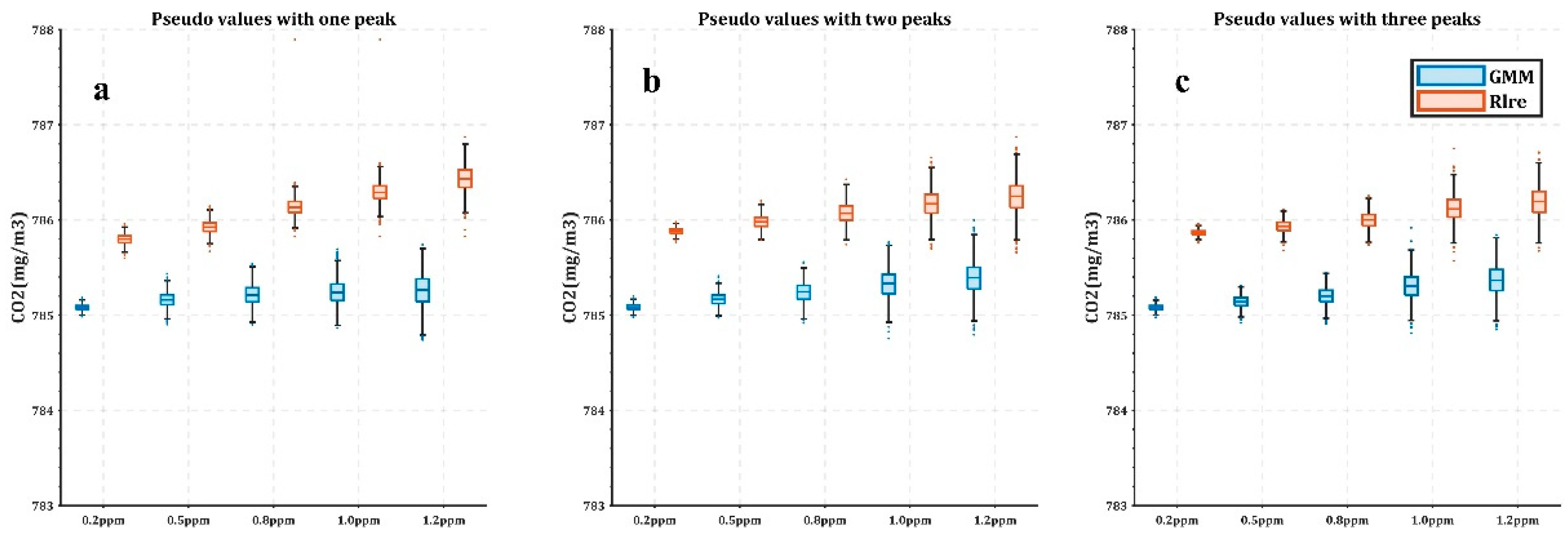
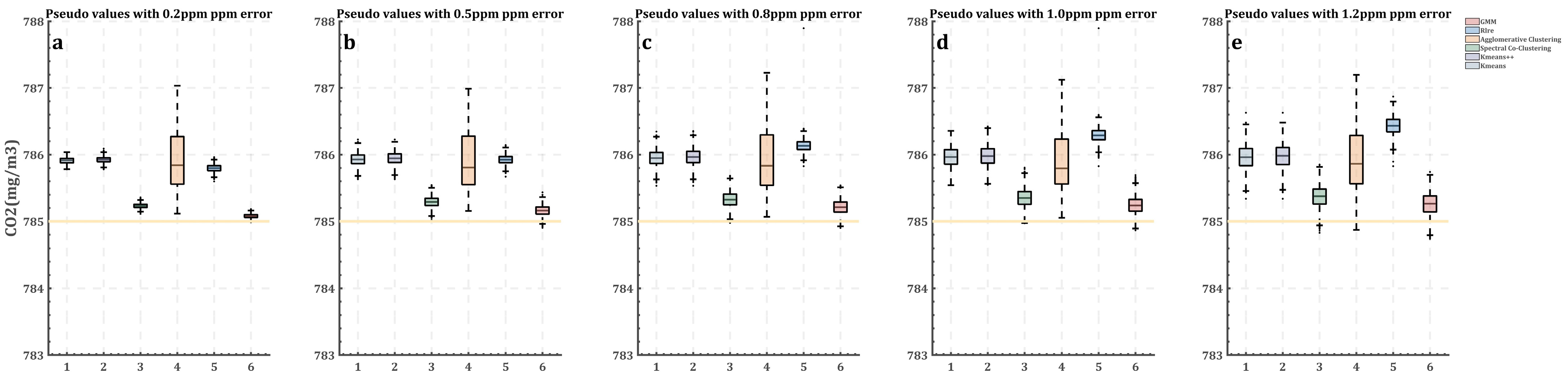
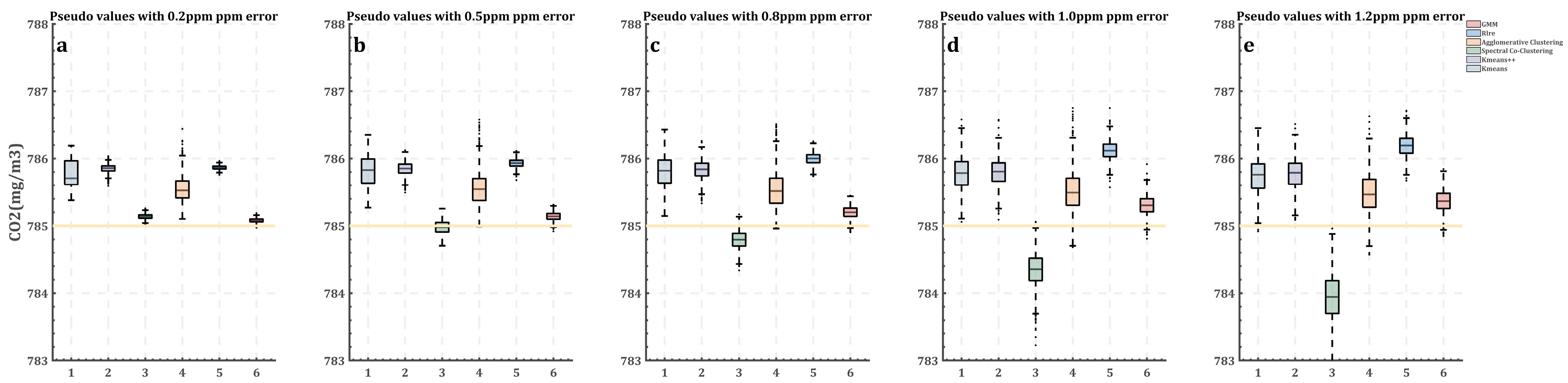
3.2. Multiple Simulation Results

To verify the validity of our method, we estimated the background CO₂ concentration for pseudo measurements containing different numbers of peaks with multiple measurement error cases (0.2 ppm, 0.5 ppm, 0.8 ppm, 1.0 ppm, 1.2 ppm). We repeated the experiment 1000 times for each set of estimates. The results of the experiments are shown in Figure 4.

Figure 4a–c represent the results of the experimental estimation of the CO₂ background concentration for pseudo measurements containing different numbers of peaks. The blue wire rod diagram represents the results of the estimation of the background concentration by the GMM in 1000 repetitions of the experiment with different measurement errors. The orange wire rod diagram represents the estimation of the CO₂ background concentration by robust local regression. We can clearly see that the GMM and robust local regression show a similar pattern for the estimation of the background concentrations, regardless of the number of peaks in the measurements. As the measurement error increases, the estimate of the background concentration deviates more from the true background concentration value. More specifically, for measurements with an error of 0.2 ppm, when using the GMM, the highest mean estimate of the background concentration is 785.08 mg/m³, which is only 0.08 mg/m³ higher than the true background concentration, while for measurements with an error of 1.2 ppm, the highest mean estimate of the background concentration is 785.39 mg/m³, which is 0.39 mg/m³ higher than the true background concentration. From this set of experiments, we can conclude that as the measurement error increases, the background observations and enhanced values fluctuate more. Some of the increased background observations caused unreasonable CO₂ enhanced values, which were not affected by the emission source, to be incorrectly considered as background measurements. Furthermore, it affects the estimation of both the robust local regression and the GMM to explain that the deviation of the background concentration from the actual value estimated by the two methods increases with the measurements error. By contrast, as the GMM estimated the background concentration in comparison to the robust local regression, the effect of more augmented values is stripped away through classification, and therefore, the GMM outperforms robust local regression in terms of the estimation.

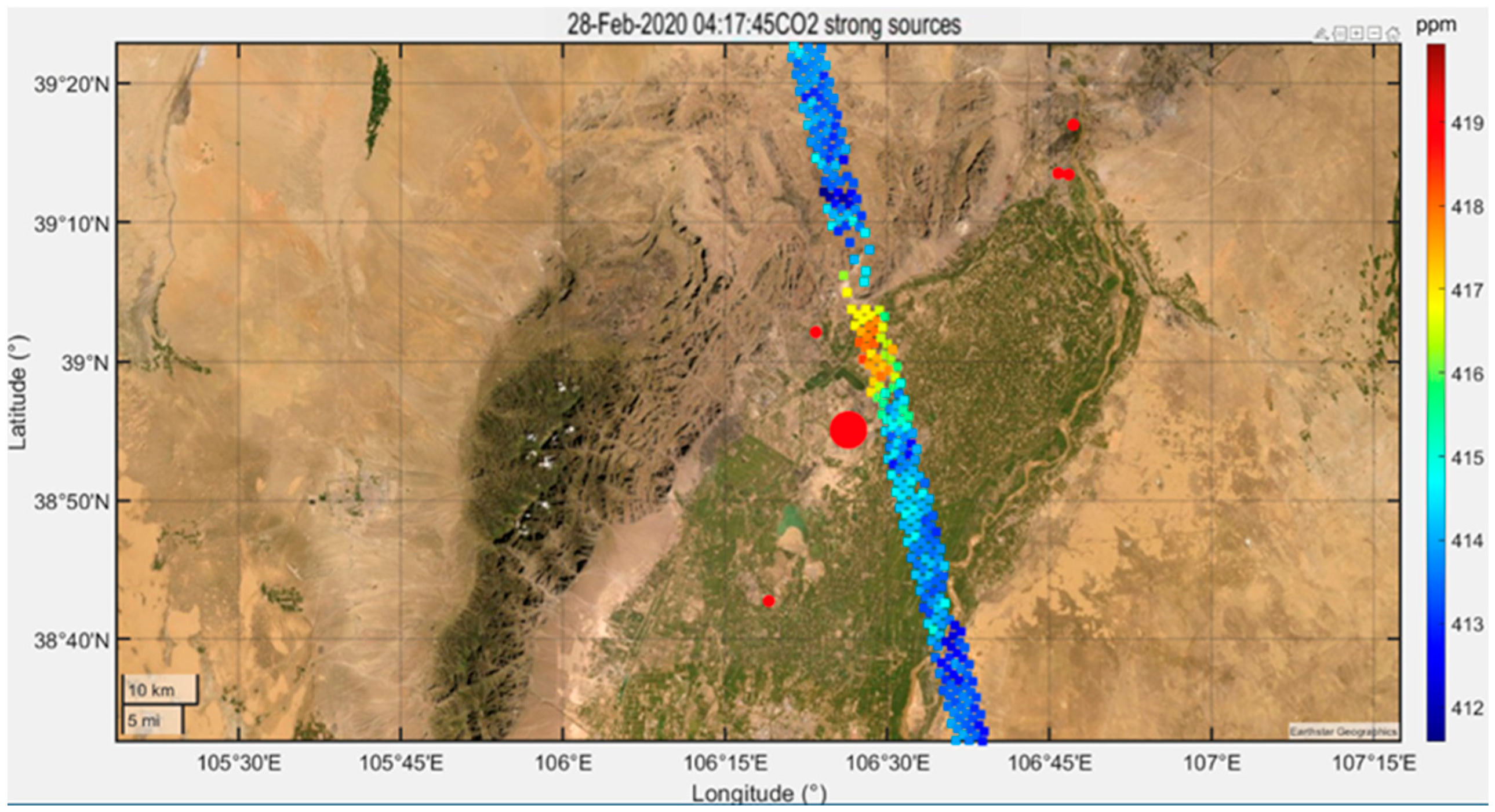
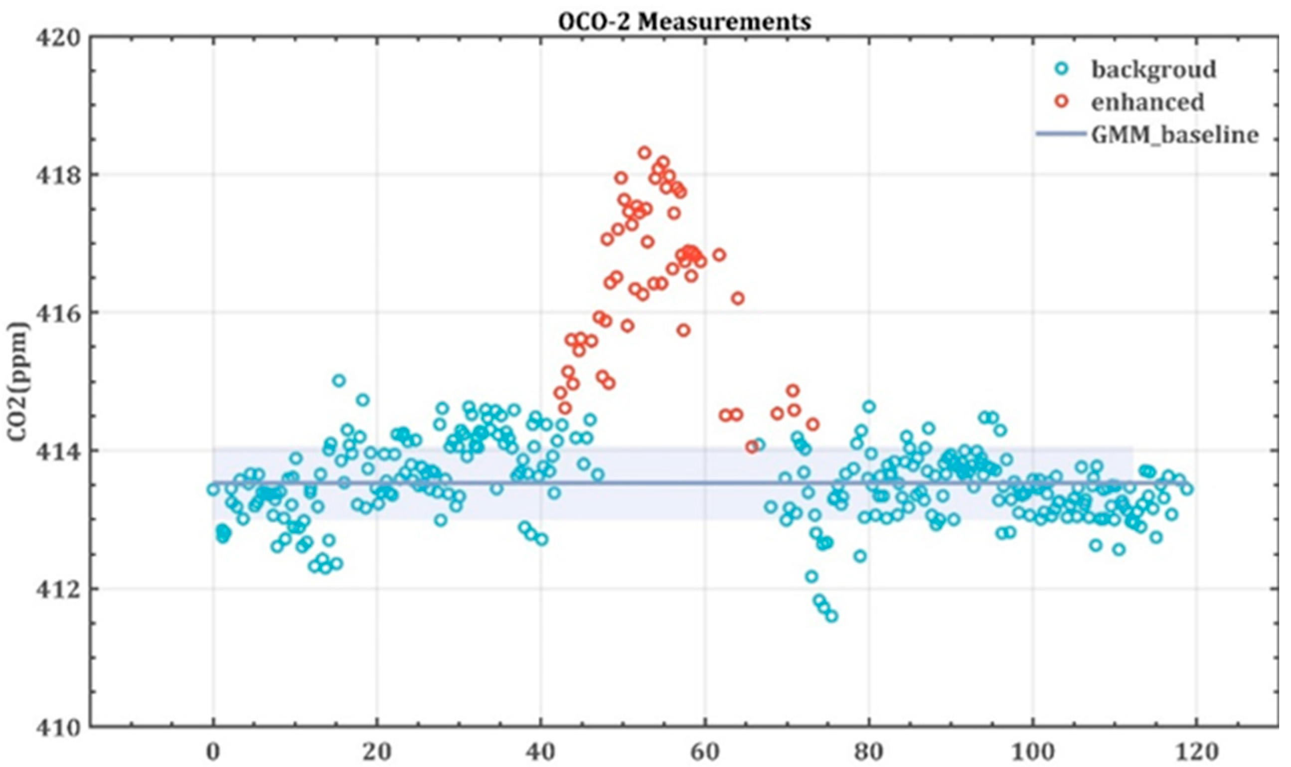
3.3. Real Experiments

To demonstrate the robustness of our algorithm, we used our method to estimate CO₂ background concentrations in different observations. The data in Figure 5 are derived from observations from the OCO-2 satellite, which quantifies the CO₂ column concentration on a given footprint by means of spectrometer observations in the O₂ band (0.758–0.772 µm), the weak CO₂ absorption band (1.594–1.619 µm), and the strong CO₂ absorption band (2.042–2.082 µm). We screened the OCO-2 observations near strong CO₂ emission sources as experimental data on 28 February 2020, where the version was v10r, the longitude was 106°15′ E to 106°40′ E, the latitude was 38°30′ N to 39°22′ N, the direction perpendicular to the wind direction was used as the positive direction of the x-axis, and the coordinates of the OCO-2 observations changed. The measurement trajectory of the data is shown in Figure 5. From Figure 6, we can clearly see that our method well separates the background concentration measurements near the strong point sources.

The data in Figure 6 were obtained from the CO₂ concentration measurements on a certain path near the source of strong CO₂ emissions using mobile equipment. The vehicle-based GHG emission monitoring system (VGMS) contains three parts: an in situ sensor (PICARRO G2201-i), a meteorological instrument, and a global positioning system (GPS). PICARRO G2201-i can sample CO₂ and CH4 simultaneously (as shown in Figure 7). For CO₂, the accuracy of the samples is ±0.2 parts per million (ppm). The meteorological instrument collects the ambient temperature, ambient pressure, ambient relative humidity, wind speed, and wind direction. The GPS records the location of the sample points on the measured track. The mobile equipment analyzes the gas along a certain path through the on-board in situ measuring instrument, and it can obtain the CO₂ concentration at a certain time. By matching with the GPS data, the CO₂ concentration in the specified geographic location can be obtained. In Figure 8, compared with the column concentration observed by satellite, the CO₂ emissions near the strong point source captured by the mobile equipment are more intense and the stripping of the background concentration from the measurements is more obvious.

4. Discussion

A variety of clustering algorithms can be used to divide observations into enhanced values and background values, such as kmeans, the spectral co-clustering algorithm, agglomerative clustering algorithm, etc. Kmeans uses the distance from the data element to the cluster center as the criterion for clustering, while kmeans++ is optimized on the basis of kmeans. The initial clustering center is determined by the principle that the clustering centers are far apart. The spectral co-clustering algorithm is an algorithm developed from graph theory. The difference between the data points is used as the weight between the data points to construct a topological network for clustering. The agglomerative clustering algorithm is a hierarchical clustering algorithm, which treats each data point as an independent cluster and continuously fuses it to the specified number of clusters. The design ideas behind these clustering algorithms are different, so their effects on classification are also quite different. Figure 9, Figure 10, and Figure 11 represent the estimation of the CO₂ background concentration by different algorithms in the case of pseudo measurements with one peak, two peaks, and three peaks, respectively, with a–e representing pseudo measurements with different observation errors, respectively. We find that, except for the agglomerative clustering algorithm, when the algorithms estimate the CO₂ background concentration, the error between the estimated value and the real value increases with the increase in the measurement error. We believe that methods of hierarchical clustering may be less applicable to such observational data. In terms of estimation performance, the GMM shows its superior ability to estimate the CO₂ background concentration, as both the absolute deviation and the root mean squared error (RMSE) exhibit good performance. Although the spectral co-clustering algorithm also delivers better estimation of the CO₂ background, it is clear that the accuracy of the estimated results degrades considerably as the number of peaks in the measurements increases. We believe this may be caused by the fact that, in the case of multiple peaks, as the measurement error increases, more biased measurements are misclassified, so the estimation of the background concentration in the final classification result only selects the value of the observation that falls. However, kmeans and kmeans++ are roughly similar in terms of their specific performance, and the performance of the CO₂ background concentration estimation is slightly better than that of the robust local regression. We believe that the reason for this phenomenon may be that, in the distance-based clustering process, some observation points with small enhancement values are also judged to be background concentration observation points, so the overall estimated effect is higher than the real background concentration value.

5. Conclusions

In this work, we propose a method that combines robust local regression and Gaussian mixture models to estimate the CO₂ background concentrations near emission sources. The method fully considers the distribution of CO₂ concentration near the emission source, so it shows a good background concentration evaluation effect in different types of CO₂ concentration measurement data. Through simulation experiments, we verified that even when the CO₂ concentration measurement error is 1.2 ppm, the CO₂ background concentration estimation error is only 0.39 mg/m³. Due to the effectiveness and simplicity of this method, the accuracy of top-down carbon emission quantification will be effectively improved in the future.

References

- Shi, T.; Han, G.; Ma, X.; Zhang, M.; Pei, Z.; Xu, H.; Qiu, R.; Zhang, H.; Gong, W. An inversion method for estimating strong point carbon dioxide emissions using a differential absorption Lidar. J. Clean. Prod. 2020, 271, 122434. [Google Scholar] [CrossRef]
- Zheng, B.; Chevallier, F.; Ciais, P.; Broquet, G.; Wang, Y.; Lian, J.; Zhao, Y. Observing carbon dioxide emissions over China’s cities and industrial areas with the Orbiting Carbon Observatory-2. Atmos. Chem. Phys. 2020, 20, 8501–8510. [Google Scholar] [CrossRef]
- Stocker, T.; Qin, D.; Plattner, G.; Tignor, M.; Allen, S.; Boschung, J.; Nauels, A.; Xia, Y.; Bex, B.; Midgley, B. Climate Change 2013: The Physical Science Basis. Contribution of Working Group I to the Fifth Assessment Report of the Intergovernmental Panel on Climate Change; IPCC: Geneva, Switzerland, 2013. [Google Scholar] [CrossRef] [Green Version]
- Wang, S.; Zhang, Y.; Hakkarainen, J.; Ju, W.; Liu, Y.; Jiang, F.; He, W. Distinguishing Anthropogenic CO2 Emissions From Different Energy Intensive Industrial Sources Using OCO-2 Observations: A Case Study in Northern China. J. Geophys. Res. Atmos. 2018, 123, 9462–9473. [Google Scholar] [CrossRef]
- Bovensmann, H.; Buchwitz, M.; Burrows, J.P.; Reuter, M.; Krings, T.; Gerilowski, K.; Schneising, O.; Heymann, J.; Tretner, A.; Erzinger, J. A remote sensing technique for global monitoring of power plant CO2 emissions from space and related applications. Atmos. Meas. Tech. 2010, 3, 781–811. [Google Scholar] [CrossRef] [Green Version]
- Cai, M.; Mao, H.; Chen, C.; Wei, X.; Shi, T. Measuring Greenhouse Gas Emissions from Point Sources with Mobile Systems. Atmosphere 2022, 13, 1249. [Google Scholar] [CrossRef]
- Shi, T.; Han, Z.; Han, G.; Ma, X.; Chen, H.; Andersen, T.; Mao, H.; Chen, C.; Zhang, H.; Gong, W. Retrieving CH 4-emission rates from coal mine ventilation shafts using UAV-based AirCore observations and the genetic algorithm–interior point penalty function (GA-IPPF) model. Atmos. Chem. Phys. 2022, 22, 13881–13896. [Google Scholar] [CrossRef]
- Cai, M.; Han, G.; Ma, X.; Pei, Z.; Gong, W. Active–passive collaborative approach for XCO2 retrieval using spaceborne sensors. Opt. Lett. 2022, 47, 4211–4214. [Google Scholar] [CrossRef]
- Shi, T.Q.; Han, G.; Ma, X.; Gong, W.; Chen, W.B.A.; Liu, J.Q.; Zhang, X.Y.; Pei, Z.P.; Gou, H.L.; Bu, L.B. Quantifying CO2 Uptakes Over Oceans Using LIDAR: A Tentative Experiment in Bohai Bay. Geophys. Res. Lett. 2021, 48, e2020GL091160. [Google Scholar] [CrossRef]
- Andersen, T.; Scheeren, B.; Peters, W.; Chen, H. A UAV-based active AirCore system for measurements of greenhouse gases. Atmos. Meas. Tech. 2018, 11, 2683–2699. [Google Scholar] [CrossRef]
- Messerschmidt, J.; Geibel, M.C.; Blumenstock, T.; Chen, H.; Deutscher, N.M.; Engel, A.; Feist, D.G.; Gerbig, C.; Gisi, M.; Hase, F.; et al. Calibration of TCCON column-averaged CO2: The first aircraft campaign over European TCCON sites. Atmos. Chem. Phys. 2011, 11, 10765–10777. [Google Scholar] [CrossRef] [Green Version]
- Kumar, P.; Broquet, G.; Caldow, C.; Laurent, O.; Gichuki, S.; Cropley, F.; Yver-Kwok, C.; Fontanier, B.; Lauvaux, T.; Ramonet, M.; et al. Near-field atmospheric inversions for the localization and quantification of controlled methane releases using stationary and mobile measurements. Q. J. R. Meteorol. Soc. 2022, 148, 1886–1912. [Google Scholar] [CrossRef]
- Liu, B.; Ma, X.; Ma, Y.; Li, H.; Jin, S.; Fan, R.; Gong, W. The relationship between atmospheric boundary layer and temperature inversion layer and their aerosol capture capabilities. Atmos. Res. 2022, 271, 106121. [Google Scholar] [CrossRef]
- Shi, T.; Han, Z.; Gong, W.; Ma, X.; Han, G. High-precision methodology for quantifying gas point source emission. J. Clean. Prod. 2021, 320, 128672. [Google Scholar] [CrossRef]
- Shi, T.Q.; Ma, X.; Han, G.; Xu, H.; Qiu, R.N.; He, B.; Gong, W. Measurement of CO2 rectifier effect during summer and winter using ground-based differential absorption LiDAR. Atmos. Environ. 2020, 220, 10. [Google Scholar] [CrossRef]
- Luo, B.; Yang, J.; Song, S.; Shi, S.; Gong, W.; Wang, A.; Du, L. Target Classification of Similar Spatial Characteristics in Complex Urban Areas by Using Multispectral LiDAR. Remote Sens. 2022, 14, 238. [Google Scholar] [CrossRef]
- Nathan, B.J.; Golston, L.M.; O’Brien, A.S.; Ross, K.; Harrison, W.A.; Tao, L.; Lary, D.J.; Johnson, D.R.; Covington, A.N.; Clark, N.N.; et al. Near-Field Characterization of Methane Emission Variability from a Compressor Station Using a Model Aircraft. Environ. Sci. Technol. 2015, 49, 7896–7903. [Google Scholar] [CrossRef]
- Andersen, T.; Vinkovic, K.; de Vries, M.; Kers, B.; Necki, J.; Swolkien, J.; Roiger, A.; Peters, W.; Chen, H.L. Quantifying methane emissions from coal mining ventilation shafts using an unmanned aerial vehicle (UAV)-based active AirCore system. Atmos. Environ.-X 2021, 12, 100135. [Google Scholar] [CrossRef]
- Fujinawa, T.; Kuze, A.; Suto, H.; Shiomi, K.; Kanaya, Y.; Kawashima, T.; Kataoka, F.; Mori, S.; Eskes, H.; Tanimoto, H. First Concurrent Observations of NO2 and CO2 From Power Plant Plumes by Airborne Remote Sensing. Geophys. Res. Lett. 2021, 48, e2021GL092685. [Google Scholar] [CrossRef]
- Xu, W.; Wang, W.; Wang, N.; Chen, B. A New Algorithm for Himawari-8 Aerosol Optical Depth Retrieval by Integrating Regional PM2.5 Concentrations. IEEE Trans. Geosci. Remote Sens. 2022, 60, 1–11. [Google Scholar] [CrossRef]
- Wunch, D.; Wennberg, P.O.; Toon, G.C.; Connor, B.J.; Fisher, B.; Osterman, G.B.; Frankenberg, C.; Mandrake, L.; O’Dell, C.; Ahonen, P.; et al. A method for evaluating bias in global measurements CO2 Total Columns Space. Atmos. Chem. Phys. 2011, 11, 12317–12337. [Google Scholar] [CrossRef] [Green Version]
- Qiu, R.; Li, X.; Han, G.; Xiao, J.; Ma, X.; Gong, W. Monitoring drought impacts on crop productivity of the US Midwest with solar-induced fluorescence: GOSIF outperforms GOME-2 SIF and MODIS NDVI, EVI, and NIRv. Agric. For. Meteorol. 2022, 323, 109038. [Google Scholar] [CrossRef]
- Qiu, R.N.; Han, G.; Ma, X.; Xu, H.; Shi, T.Q.; Zhang, M. A Comparison of OCO-2 SIF, MODIS GPP, and GOSIF Data from Gross Primary Production (GPP) Estimation and Seasonal Cycles in North America. Remote Sens. 2020, 12, 258. [Google Scholar] [CrossRef] [Green Version]
- Nassar, R.; Moeini, O.; Mastrogiacomo, J.-P.; O’Dell, C.W.; Nelson, R.R.; Kiel, M.; Chatterjee, A.; Eldering, A.; Crisp, D. Tracking CO2 emission reductions from space: A case study at Europe’s largest fossil fuel power plant. Front. Remote Sens. 2022, 3. [Google Scholar] [CrossRef]
- Nassar, R.; Mastrogiacomo, J.P.; Bateman-Hemphill, W.; McCracken, C.; MacDonald, C.G.; Hill, T.; O’Dell, C.W.; Kiel, M.; Crisp, D. Advances in quantifying power plant CO2 emissions with OCO-2. Remote Sens. Environ. 2021, 264, 112579. [Google Scholar] [CrossRef]
- Nassar, R.; Hill, T.G.; McLinden, C.A.; Wunch, D.; Jones, D.B.A.; Crisp, D. Quantifying CO2 Emissions From Individual Power Plants From Space. Geophys. Res. Lett. 2017, 44, 10045–10053. [Google Scholar] [CrossRef] [Green Version]
- Pei, Z.P.; Han, G.; Ma, X.; Shi, T.Q.; Gong, W. A Method for Estimating the Background Column Concentration of CO2 Using the Lagrangian Approach. IEEE Trans. Geosci. Remote Sens. 2022, 60, 1–12. [Google Scholar] [CrossRef]
- Pei, Z.P.; Han, G.; Ma, X.; Su, H.; Gong, W. Response of major air pollutants to COVID-19 lockdowns in China. Sci. Total Environ. 2020, 743, 140879. [Google Scholar] [CrossRef]
- Ruckstuhl, A.F.; Jacobson, M.P.; Field, R.W.; Dodd, J.A. Baseline subtraction using robust local regression estimation. J. Quant. Spectrosc. Radiat. Transf. 2001, 68, 179–193. [Google Scholar] [CrossRef]
- Krishna, K.; Murty, M.N. Genetic K-means algorithm. IEEE Trans. Syst. Man Cybern. Part B Cybern. 1999, 29, 433–439. [Google Scholar] [CrossRef]
- Dhillon, I.S. Co-clustering documents and words using bipartite spectral graph partitioning. In Proceedings of the Seventh ACM SIGKDD International Conference on Knowledge Discovery and Data Mining, San Francisco, CA, USA, 26–29 August 2001; pp. 269–274. [Google Scholar]
- Murtagh, F.; Legendre, P. Ward’s hierarchical agglomerative clustering method: Which algorithms implement Ward’s criterion? J. Classif. 2014, 31, 274–295. [Google Scholar] [CrossRef] [Green Version]
- Reynolds, D.A. Gaussian mixture models. Encycl. Biom. 2009, 741, 827–832. [Google Scholar]
- Moon, T.K. The expectation-maximization algorithm. IEEE Signal Process. Mag. 1996, 13, 47–60. [Google Scholar] [CrossRef]
Disclaimer/Publisher’s Note: The statements, opinions and data contained in all publications are solely those of the individual author(s) and contributor(s) and not of MDPI and/or the editor(s). MDPI and/or the editor(s) disclaim responsibility for any injury to people or property resulting from any ideas, methods, instructions or products referred to in the content. |
© 2023 by the authors. Licensee MDPI, Basel, Switzerland. This article is an open access article distributed under the terms and conditions of the Creative Commons Attribution (CC BY) license (https://creativecommons.org/licenses/by/4.0/).
Share and Cite
Sun, Q.; Chen, C.; Wang, H.; Xu, N.; Liu, C.; Gao, J. A Method for Assessing Background Concentrations near Sources of Strong CO2 Emissions. Atmosphere 2023, 14, 200. https://doi.org/10.3390/atmos14020200
Sun Q, Chen C, Wang H, Xu N, Liu C, Gao J. A Method for Assessing Background Concentrations near Sources of Strong CO2 Emissions. Atmosphere. 2023; 14(2):200. https://doi.org/10.3390/atmos14020200
Chicago/Turabian StyleSun, Qingfeng, Cuihong Chen, Hui Wang, Ningning Xu, Chao Liu, and Jixi Gao. 2023. "A Method for Assessing Background Concentrations near Sources of Strong CO2 Emissions" Atmosphere 14, no. 2: 200. https://doi.org/10.3390/atmos14020200