Computation of the Attenuated Backscattering Coefficient by the Backscattering Lidar Signal Simulator (BLISS) in the Framework of the CALIOP/CALIPSO Observations

Abstract

This paper presents the Backscattering Lidar Signal Simulator (BLISS), an end-to-end lidar simulator developed by the Centre National d’Etudes Spatiales (CNES). We computed the constant multiple-scattering (MS) coefficient of BLISS with a Monte Carlo (MC) code in the framework of CALIOP/CALIPSO observations for different homogeneous and plane-parallel stratocumulus and cirrus cloud geophysical scenes. The MS coefficient varies from 0.46 to 0.63. Then we evaluated the Level 1 products of BLISS. Above and in-cloud relative difference between the attenuated backscattering coefficient vertical profile simulated by BLISS and by the MC code is smaller than 0.5% under single-scattering regime and smaller than 10% (30% if optical depth of cirrus is large) under multiple-scattering regime, thus confirming the robustness of BLISS.

1. Introduction

Clouds play a major role in the Earth climatic system energy balance [1]. For example, liquid and opaque low-level clouds (i.e., stratocumulus) efficiently reflect solar radiation back to space and contribute to cooling the Earth’s surface whereas iced and transparent high-level clouds (cirrus) strongly absorb surface thermal radiation and re-emit it back to the ground, leading to warming [2]. Overall, clouds contribute to cooling the Earth’s climatic system [3,4]. In the context of climate change, it is important to know accurately the spatio-temporal distribution of clouds [5], especially since their feedback, positive, is always quite uncertain [6].

Spaceborne sensors are suitable tools to infer clouds properties at the global scale [7,8,9]. Among the remote sensing techniques, active sounding plays an important role because it allows access to the vertical distribution of cloud properties [10]. Over the last decade, the Cloud–Aerosol Lidar and Infrared Pathfinder Satellite Observations (CALIPSO) [11] have improved our understanding of the spatial distribution of microphysical and optical properties of clouds and aerosols [12]. Future missions are planned to pursue those observations. For example, the Earth Clouds, Aerosol, and Radiation Explorer (EarthCARE) [13] scheduled for 2023 will deploy a high spectral resolution (HSR) lidar in space [14].

Evaluating the performance of lidar systems [15,16], developing cloud products retrieval algorithms [17,18,19,20,21], or assimilating lidar observations [22,23,24] is generally based on the direct simulation of the lidar signal. Such a lidar forward operator must consider all the technical characteristics of the lidar system, the microphysical and optical properties of the cloudy geophysical scenes, and the multiple-scattering (MS) radiative process [25]. Monte Carlo (MC) calculations are rather straightforward, and were widely used to investigate the MS effects on lidar signal [25,26,27,28]. Nevertheless, MC calculation of MS lidar signals are slow and time-consuming. Therefore, a lidar forward operator based on MS approximate models are widely employed in the operational context. For example, in the DARDAR (for liDAR/raDAR) cloud retrieval algorithm [19], the fast approximate model of [29] can be referenced. In the Z (reflectivity) Model for Variational assimilation (ZmVar) of the European Centre for Medium Range Weather Forecasts (ECMWF) the Photon Variance–Covariance (PVC) method [30] or the “Platt approximation” [31] can be chosen [32]. The “Platt approximation” is also used in the lidar simulator [33,34] of the Cloud Feedback Model Intercomparison Project (CFMIP) Observation Simulator Package (COSP) [35,36] and in the CALIOP cloud products [20,21]. The “Platt approximation” is one of the easiest methods to implement [30]. Indeed, it only requires defining a multiple-scattering coefficient to be assigned in the single-scattering lidar equation. At the same time, this multiple-scattering coefficient is a function of the multitude of parameters (system lidar technical characteristics, optical and geometrical properties of cloudy geophysical scenes) and need to be carefully evaluated [28].

The main purpose of this paper is to present the Backscattering Lidar Signal Simulator (BLISS), an end-to-end simulator developed by the Centre National d’Etudes Spatiales (CNES), which simulates the return signal received by a backscattering airborne or spaceborne lidar and its associated retrieved products for a given geophysical scene defined by the user. MS is based on the “Platt approximation”. Computation of the MS coefficient of BLISS and validation of outputs of BLISS in the framework of the CALIOP/CALIPSO framework for different cloudy (stratocumulus and cirrus) scenes were performed with the help of the Monte Carlo Radar Lidar (McRALI) software developed at the Laboratoire de Météorologie Physique [37,38].

The organization of this paper is as follows: The methodology, the BLISS simulator, and conditions of simulation are presented in Section 2. The McRALI simulator is briefly presented as well. Section 3 is devoted to the main results. In the first part, the multiple-scattering coefficient is computed with the McRALI simulator. Then, in the second part outputs of BLISS and McRALI simulators for identical cloudy geophysical scenes are compared. Finally, in Section 4 we discuss the validation of the BLISS simulator and future research directions are highlighted.

2. Materials and Methods

2.1. General Principles for Computation of Lidar Backscatterred Signal under Multiple-Scattering Regime

The basic lidar equation under the single-scattering condition can be written as [39]:

$$p\left(r\right)=\frac{K\left(r\right)}{r^2}\beta \left(r\right)\exp \left[-2{{\displaystyle \int }}_0^r\alpha \left(r\right)dr\right]$$

(1)

where $p$ is the received power on the detector from range $r$ (in m), $K$ is the instrument function, $\alpha$ (in m⁻¹) is the extinction, and $\beta$ (in m⁻¹ sr⁻¹) is the backscattering coefficient defined as $\beta =P\left(\pi \right){\sigma }_s$ where $P\left(\pi \right)$ (in sr⁻¹) is the scattering phase function in the backward direction and ${\sigma }_s$ (in m⁻¹) is the scattering coefficient.

We use the notations of the work by [28], the function $S_1\left(r\right)$ characterizes lidar signals in the single-scattering (SS) approximation (corrected for the offset and instrumental factors):

$$S_1\left(r\right)=\left[{\beta }_p\left(r\right)+{\beta }_m\left(r\right)\right]·T^2\left(r\right)$$

(2)

where ${\beta }_p\left(r\right)$ and ${\beta }_m\left(r\right)$ represent the backscattering coefficient of particles and atmospheric molecules; $T^2\left(r\right)=T_m^2\left(r\right)·T_p^2\left(r\right)$ is the two-way transmittance from the lidar to the range $r$, $T_m^2\left(r\right)$ and $T_p^2\left(r\right)$ are the molecular and the particulate transmittances, respectively.

The term “apparent attenuated backscatter” or the term “apparent backscatter” (see, e.g., [30,40]) is employed for lidar signals $S_{MS}\left(r\right)$ computed in multiple-scattering conditions (corrected for the offset and instrumental factors). It is also called the attenuated backscattering coefficient, hereafter also denoted as ATB. It can be written as

$$S_{MS}\left(r\right)=G_{MS}\left(r\right)·\left[{\beta }_p\left(r\right)+{\beta }_m\left(r\right)\right]·T_m^2\left(r\right)·T_p^2\left(r\right)$$

(3)

where the multiple-scattering (MS) function $G_{MS}\left(r\right)$ is the ratio

$$G_{MS}\left(r\right)=\frac{S_{MS}\left(r\right)}{S_1\left(r\right)}$$

(4)

employed as a factor that corrects the lidar of the SS approximation. In that case, according to [31,41], lidar signals can be written [42] as

$$S_{MS}\left(r\right)=\left[{\beta }_p\left(r\right)+{\beta }_m\left(r\right)\right]·T_m^2\left(r\right)·T_p^2\left(r\right)·\exp \left\{2\left[1-{\eta }_{MS}\left(r\right)\right]{\tau }_p\left(r\right)\right\}$$

(5)

where ${\tau }_p\left(r\right)$ is the in-cloud optical depth. ${\eta }_{MS}\left(r\right)$ is the multiple-scattering function that can be rewritten [42]

$${\eta }_{MS}\left(r\right)=1-\frac{1}{2·{\tau }_p\left(r\right)}·\ln \left[G_{MS}\left(r\right)\right]$$

(6)

The constant multiple-scattering coefficient ${\eta }_{MS}$ was proposed by [31] to account for “secondary scattering or higher order processes”. In the work [41], ${\eta }_{MS}\left(r\right)$ was defined as the factor that multiplies the optical depth. It has a value less than unity and may vary with altitude. However, a constant coefficient ${\eta }_{MS}$ is largely used in works where profiles of cloud parameters are retrieved from lidar data (see e.g., [20]). Accordingly, computation of the ATB by BLISS (see below) is based on the use of ${\eta }_{MS}=const$. Values of ${\eta }_{MS}$ are estimated using computations of $G_{MS}$ by McRALI as a function of cloudy geophysical scenes.

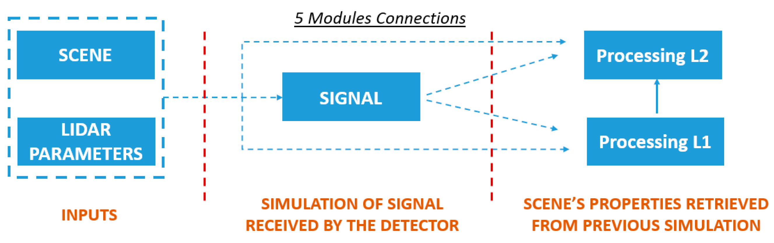
2.2. Presentation of BLISS

BLISS is an end-to-end simulator developed by CNES. We talk about end-to-end simulation because it allows the simulation of the measurements (i.e., Level 0 and Level 1 products) and the retrieval (i.e., Level 2) with dedicated data management systems. An end-to-end simulator can build a virtual observing system. It is also able to retrieve geophysical properties from its synthetic observations or from real observations. Such an end-to-end simulator leads to test the processor chain from Level 0 to Level 2, to assess the performance of the measurement system with respect to random and systematic error, to perform sensitivity studies to optimize instrumentation setting and retrieval algorithms and, more generally, to validate measurements of the scientific mission. BLISS simulates the backscattered signal received by a backscattering airborne or spaceborne lidar and the associated retrieved products for a given geophysical scene defined by the user. It enables quick assessment of expected performances of future spaceborne lidar missions. The instrument radiometric noise is modeled with a normal law. Simple backscattering lidars, polarization measurements, and high spectral resolution lidars (HSRL) can be modeled. The software outputs consist of Level 1 products (attenuated backscatter or ATB and scattering ratio profiles) and Level 2 products (extinction and backscattering profiles, depolarization, and lidar ratio depending on the modeled lidar system).

BLISS consists of five different and interconnected modules: the lidar parameters, the scene, the signal, the processing L1 and the processing L2 modules. Figure 1 shows their connections. The lidar parameters module allows defining transmitter, receiver, and detector characteristics, as well as mission specificities (altitude, line of sight and so on). The Scene module allows defining the scene observed by the lidar (atmosphere, aerosols, clouds, and surface characteristics). Aerosols and clouds properties can either be defined by the user or chosen in an internal database based on the Optical Properties of Aerosols and Clouds (OPAC) database as described in [43]. Some oceanic properties can also be defined [44]. The signal module computes and bins optical powers backscattered towards the detector using the lidar equations described in [39]. In a simple backscatter lidar configuration, the power $p\left(r\right)$ simulated at range $r$ by the BLISS simulator is provided by:

$$p\left(r\right)=\frac{K\left(r\right)}{r^2}\left[{\beta }_{mol}\left(r\right)+{\beta }_{part}\left(r\right)\right]\exp \left\{-2{{\displaystyle \int }}_0^r\left[{\alpha }_{mol}\left(r\right)+\epsilon \ast {\alpha }_{part}\left(r\right)\right]dr\right\}$$

(7)

where $K$ is the instrument function (depending on the laser energy, the receiver telescope surface or the instrumental transmission for instance), ${\beta }_{mol}$ is the molecular backscattering coefficient, ${\beta }_{part}$ is the particle backscattering coefficient, ${\alpha }_{mol}$ is the molecular extinction, ${\alpha }_{part}$ is the particulate extinction and $\epsilon$ is the multiple-scattering coefficient for particles. In the version of BLISS used for this paper, this coefficient is constant over the range considered for a given view. Then, $p\left(r\right)$ is converted into the number of photoelectrons measured by the detector, depending on the lidar optical transmission and detector efficiency. This module also allows to compute the solar background and radiometric noises (though these quantities were not used in this study and are therefore not be further developed here). The processing L1 module computes Level 1 products, which are the direct measurements corrected for the instrument characteristics, from the powers computed in the signal module. Depending on the lidar type, these can be the ATB or the Attenuated Molecular Backscatters (AMBs) and the Attenuated Particular Backscatter (APB). They can also depend on the polarization. These products are all described in [39]. The formula for the ATB is provided hereafter:

$$ATB\left(r\right)=p\left(r\right)\frac{r^2}{K\left(r\right)}=\left[{\beta }_{mol}\left(r\right)+{\beta }_{part}\left(r\right)\right]\exp \left\{-2{{\displaystyle \int }}_0^r\left[{\alpha }_{mol}\left(r\right)+\epsilon \ast {\alpha }_{part}\left(r\right)\right]dr\right\}$$

(8)

This module also computes the value of AMB using theoretical values of ${\beta }_{mol}\left(r\right)$. In the BLISS simulator, this calculation can be performed either by using the same molecular profile, which has been used in the scene module, or by using a different profile for the inversion. Finally, the processing L2 module computes the Level 2 products depending on the lidar type selected (simple backscattering lidar or HSR lidar). These products can be scattering and depolarizing ratios, optical depths and backscattering, extinction and depolarization coefficient profiles. For the simple backscattering lidar, the retrieval algorithm is based on Klett approach as described in [39]. In this case, it is necessary to provide the vertical profile of lidar ratio as an input characteristic. The BLISS version used in this document is the V2.8.

2.3. Presentation of McRALI

We briefly recall the functional characteristics of McRALI. The lidar signals $S_{MS}\left(r\right)$ and $S_1\left(r\right)$ are computed with the McRALI software developed at the Laboratoire de Météorologie Physique [37,38]. The software employs a forward MC approach along with the locate estimate method to simulate propagation of radiation (see, e.g., [45]). McRALI is based on the 3DMCPOL model [46]. The polarization state of the radiation is computed using Stokes vectors and scattering matrices of atmospheric compounds. It takes into account molecular scattering. McRALI is a fully 3D software. Values of the extinction coefficients, the single-scattering albedos, and the scattering matrices are assigned in 3D-space. The position of a lidar can be anywhere within or outside of the atmosphere, that is spaceborne-, airborne-, and ground-based measurement conditions can be simulated [28]. A user can assign a lidar beam direction, a receiver field-of-view (FOV), a Stokes vector, and a divergence for the emitted light.

2.4. Conditions of Simulations

In order to simulate the ATB as measured by CALIOP/CALIPSO, the lidar altitude, the full FOV, and the full laser divergence are assigned in the McRALI to 705 km, 130 µrad, and 100 µrad, respectively. The lidar beam direction is nadir-viewing. The vertical spatial resolution is 20 m, which is close to the smallest vertical resolution (30 m) of the CALIOP Level 1 data product [47].

Vertical molecular extinction ${\alpha }_m$ is computed on the base of the work by [48] and is provided by ${\alpha }_m\left(z\right)=\left[{\tau }_m\left(z\right)-{\tau }_m\left(z+\Delta z\right)\right]/\mathsf{\Delta }z$ where $z$ is the altitude, $\Delta z$ the vertical spatial resolution and ${\tau }_m$ is the molecular optical depth provided by ${\tau }_{mol}\left(z\right)={\tau }_{mol}\left(0\right)P\left(z\right)/P\left(0\right)$ where $P\left(z\right)$ is the vertical profile of pressure. Optical depth at $z=0$ is provided by ${\tau }_{mol}\left(0\right)=c_1\left(1.0+c_2/{\lambda }^2+c_3/{\lambda }^4\right)/{\lambda }^4$ where $c_1=0.008569$, $c_2=0.0113$ and $c_3=0.00013$. $\lambda$ is the wavelength in μm. The vertical profile of pressure is provided by $P\left(z\right)=P\left(0\right)\exp \left(-z/8\right)$ where $P\left(0\right)=1013.25$ hPa.

Simulations of this work were performed for four types of particles, namely two types of warm and liquid cloud (stratocumulus) and two types of cold and iced cloud (cirrus) with different effective radius ($R_{eff}$) and extinction coefficient. Because Monte Carlo methods are very time consuming, our study was restricted to the case of the plane-parallel homogenous layer placed within the altitude range of 1.0–1.3 km for stratocumulus cloud and 8.0–11.0 km for the cirrus cloud.

Optical properties of particles (phase function, extinction, single-scattering albedo) were computed at the wavelength 0.532 µm. Stratocumulus phase functions were computed according to the Mie theory for water spheres having gamma size distributions with $R_{eff}=3.0 \mathsf{\mu }\mathrm{m}$ and $R_{eff}=9.0 \mathsf{\mu }\mathrm{m}$ (the standard deviation is 0.3 µm). Cirrus optical properties are those used in the work of [28]. They were computed using the Improved Geometric Optics Method [49], assuming that cirrus have gamma size distribution; the particles are assumed to be hexagonal ice crystals having deeply rough surface of the facets, representative of a jet-stream cirrus with $R_{eff}=28.4$ µm (the standard deviation is 10.05 µm) and of a cirrus cloud with $R_{eff}=40.0$ µm (the standard deviation is 12.25 µm). Figure 2 shows the four phase functions used in this study. Their different behaviours at forward and backward angles can be seen in the insets.

Simulations were performed for four values of the extinction (1, 3, 5, and 10 km⁻¹) for stratocumulus and three values of the extinction (0.05, 0.2, 1.0 km⁻¹) for cirrus clouds.

3. Results

3.1. Estimation of the BLISS Multiple-Scattering Coefficient with McRALI

Computation of the ATB by BLISS is based on the use of ${\eta }_{MS}\left(d\right)$ (see Equation (6)) where $d$ is the in-cloud distance from the top of clouds. Figure 3 shows ${\eta }_{MS}\left(d\right)$ estimated by McRALI for all the geophysical scenes. Concerning stratocumulus fields, ${\eta }_{MS}$ varies from 0.45 to 0.65. ${\eta }_{MS}$ is approximately 0.1 smaller for an effective radius of 3 µm than for an effective radius of 9 µm meaning that multiple scattering is more important for small particles. ${\eta }_{MS}$ decreases (increases) slightly by about 0.05 with $d$ if extinction is larger (smaller) than about 3 to 5 km⁻¹. Concerning cirrus fields, ${\eta }_{MS}$ varies from 0.3 to 0.65. ${\eta }_{MS}$ is slightly smaller by about 0.05 for effective radius of 40.0 µm than for an effective radius of 28.4 µm. ${\eta }_{MS}$ increases with $d$ but no larger than 0.2. One can note that values of ${\eta }_{MS}\left(d\right)$ computed in this work are consistent with those found in [28].

The multiple-scattering coefficient ${\eta }_{MS}\left(d\right)$ is a function of the in-cloud distance $d$ (see Figure 3a,b). However, the multiple-scattering coefficient value is assumed to be constant in BLISS. To define the multiple-scattering coefficient to be used in BLISS, we define the error function $f\left(\eta \right)$ between ATB simulated by BLISS and McRALI as follows:

$$f\left(\eta \right)={\displaystyle \sum }_{i=1}^N\left|1-\frac{AT{B}_{BLISS}\left(\eta ,d_i\right)}{AT{B}_{McRALI}\left(d_i\right)}\right|$$

(9)

where the in-cloud distance $d_i=i·\mathsf{\Delta }h$ with the step $\Delta h=20$ m for stratocumulus and $\Delta h=100$ m for cirrus and $i=1,\dots ,N$ with $i=1$ the first layer and $i=N$ the last layer. The value ${\eta }_0$ that minimizes Equation (9) is the (constant) multiple-scattering coefficient value used in BLISS. The values of ${\eta }_0$ are shown in

Table 1. Multiple-scattering coefficient ${\eta }_0$ used in BLISS for stratocumulus and cirrus clouds.

Stratocumulus Cloud				Cirrus Cloud
Extinction (km−1)	Optical Depth	${\mathit{\eta }}_0$ (${\mathit{R}}_{\mathit{e}\mathit{f}\mathit{f}}=3$ μm)	${\mathit{\eta }}_0$ (${\mathit{R}}_{\mathit{e}\mathit{f}\mathit{f}}=9$ μm)	Extinction (km−1)	Optical Depth	${\mathit{\eta }}_0$ (${\mathit{R}}_{\mathit{e}\mathit{f}\mathit{f}}=28.4$ μm)	${\mathit{\eta }}_0$ (${\mathit{R}}_{\mathit{e}\mathit{f}\mathit{f}}=40.0$ μm)
1	0.3	0.56	0.63	0.05	0.15	0.57	0.52
3	0.9	0.54	0.61	0.2	0.6	0.55	0.53
5	1.5	0.51	0.56	1.0	3.0	0.53	0.48
10	3.0	0.46	0.53

.

For stratocumulus, the values of ${\eta }_0$ are between 0.46 and 0.63 and increase about 0.06 with effective radius from 3 µm to 9 µm. For cirrus, the values of ${\eta }_0$ are between 0.48 and 0.57 but decrease about 0.04 with effective radius increasing from 28.4 µm to 40 µm. Both cirrus and stratocumulus ${\eta }_0$ decreases with the cloud vertical optical depth.

3.2. Comparison of ATB Simulated by BLISS and McRALI in Multiple-Scattering Regime

Vertical profiles of ATB computed by BLISS and by McRALI in the SS and MS regimes for stratocumulus ($R_{eff}=9$ µm) and cirrus clouds ($R_{eff}=28.4$ µm) are shown in Figure 4 and Figure 5, respectively. The vertical profiles of the ATB relative error, defined as $\left(AT{B}_{McRALI}-AT{B}_{BLISS}\right)/AT{B}_{BLISS}$ between ATB computed by BLISS and McRALI in SS and MS regimes for all geophysical scenes are shown in Figure 6. We note that for BLISS simulations in SS regime, ${\eta }_0$ value is always set to 1, whereas in MS regime ${\eta }_0$ values are set according to values presented in Table 1.

In SS regime, vertical profiles of ATB computed by BLISS and by McRALI are very close for all geophysical scenes, although BLISS and McRALI use fundamentally different computation methods. ATB relative error is smaller than 0.5% above and within the cloud, and smaller than 3% under the cloud.In MS regime and for stratocumulus cloud, vertical profiles of ATB computed by BLISS and by McRALI are very close above and within the cloud. ATB relative error is smaller than 3%. Below the cloud, larger ATB relative errors are visible leading to relative errors up to 100% for the largest extinction coefficient. For cirrus cloud, ATB maximal relative error is 10% for extinction smaller than 0.2 km⁻¹ (i.e., optical depth smaller than 0.6) and 30 % for the large extinction (optical depth around 3). As shown in Section 3.1, ${\eta }_{MS}$ varies within a range of 0.05 and 0.2 with the in-cloud distance for stratocumulus and cirrus, respectively. This is consistent with the fact that the ATB relative error is larger for cirrus clouds than for stratocumulus clouds. Under the cirrus clouds, ATB relative error can greatly exceed 100% and is not shown in the figure.

4. Discussion

We investigated the performance of BLISS to simulate, in multiple-scattering regime, the vertical profile of the ATB in the framework of CALIOP/CALIPSO observations. The simulation experiments were carried out with a homogeneous plane-parallel cloud. Because MC computations are very time-consuming, we restricted our study to stratocumulus and cirrus with a typical thickness of 300 m and 3 km but with optical properties (optical depth, effective radius, and phase function) varying sufficiently so that they are representative of wide range of clouds.

In the first step, the multiple-scattering coefficient ${\eta }_{MS}$ were computed with the help of the McRALI lidar code. As expected, ${\eta }_{MS}$ is the function of the in-cloud depth and of the effective radius [28,34]. ${\eta }_{MS}$ varies from 0.45 to 0.65 and from 0.3 to 0.65 for stratocumulus and cirrus, respectively. In the version V2.8 of BLISS, the multiple-scattering coefficient is assumed to be constant. We defined the constant multiple-scattering coefficient ${\eta }_0$ in such a way that the in-cloud vertically integrated relative difference between the ATB computed by BLISS and McRALI is minimal. We found that ${\eta }_0$ varies from 0.46 to 0.63 and from 0.48 to 0.57 for stratocumulus and cirrus, respectively, and that ${\eta }_0$ decreases with vertical optical depth for both. ${\eta }_0$ increases (decreases) by about 0.05 with effective radius for stratocumulus (cirrus) varying from 3 to 9 µm (to 28.4 to 40 µm).

In the second step, we analyzed the vertical profiles of the relative difference between ATB computed by BLISS with the new multiple-scattering coefficient and by McRALI. First, we confirmed the robustness of the BLISS simulator in SS regime. Indeed, for all cloudy geophysical scenes, maximal ATB relative error is smaller than 0.5% above and within the cloud, and smaller than 3% under the cloud. Afterward, we highlighted that, in MS regime, BLISS simulator is very efficient. Indeed, the maximal in-cloud ATB relative error is smaller than 3% for stratocumulus and 10% for cirrus (30% if optical depth of cirrus is very large, around 3). At the same time, it should be noted that ATB relative error under clouds can be very large.

Several studies have already indicated values for the constant multiple-scattering coefficient $\eta$ to be used for cirrus cloud in the framework of CALIOP observations. Based on Monte Carlo analysis, the value of $\eta$ is suggested to be between 0.6 and 0.8 in the work [42]. COSP simulator is based on the lidar simulator ActSim, for which the works [50] and [51] proposed $\eta =0.5$. In COSP1 and COSP2 [35,36], $\eta$ is assigned to 0.7 [33] but [34] showed that a value of $\eta$ between 0.5 and 0.6 is better. Based on infrared sounder and CALIPSO data, the work [52] proposed $\eta$ between 0.35 and 0.55 depending on cloud emissivity. From combined radar and CALIOP data, the work [53] found $\eta$ values around 0.61. In CALIOP cloud products up to version 3, $\eta$ is set to 0.6, whereas for version 4 a temperature-dependent coefficient is used, as suggested by [54], which varied in between 0.46 and 0.78 [20,21,55]. Based on the PVC approximation to account for MS, [32] also estimated that $\eta$ increases with temperature, from 0.55 at 220 K to 0.75 at 290 K. For warm liquid cloud, [34] showed that a value of $\eta$ between 0.4 and 0.6 is a good candidate, depending of optical depth and effective radius. Based on detailed and accurate Monte Carlo analysis, [28] provided an estimation of the multiple-scattering coefficient that varies from 0.25 to 0.75 as a function of in-cloud depth.

Although all these studies indicate that the multiple-scattering coefficient can vary in a wide range, the constant multiple-scattering coefficient ${\eta }_0$ estimated in our work is rather consistent with previous published values. According to [21,32] it should be better to parametrize ${\eta }_0$ as a function of temperature. In order to make the BLISS lidar forward operator more accurate, the multiple-scattering coefficient should also be function of the in-cloud depth $d$, of optical depth, and effective radius. Such parametrization is difficult to obtain. It would be easier to implement the expression of multiple-scattering coefficient ${\eta }_{MS}\left(d\right)$ provided in [28]. This aspect will be studied in future work with the version V2.12 of BLISS, which is planned to take into account the variation in the multiple-scattering coefficient with the in-cloud depth.

Another point must also be addressed: as noted in this study the ATB relative error under clouds can be larger than 100%. As it can impact the signal in case of multi-layer clouds, it is important to evaluate the MS effects on lidar signal in these cases. Finally, as noted in the Section 2.2, BLISS can deal with some application for inferring cloud properties (i.e., Level 2 products). This topic will be the purpose of another paper.

5. Conclusions

This paper presents BLISS, an end-to-end simulator developed by the CNES which simulates the return signal received by a backscattering airborne or spaceborne lidar and its associated retrieved products for a given geophysical scene defined by the user. The software outputs consist of Level 1 products (attenuated backscatter or ATB and scattering ratio profiles) and Level 2 products (extinction and backscattering profiles, depolarization, and lidar ratio depending on the modeled lidar system).

According to several simulations for different cloudy geophysical scenes, the MC code McRALI is used to set up the MS coefficient of the BLISS lidar forward model. The MS coefficient varies from 0.46 to 0.63. Above and in-cloud relative difference between the ATB vertical profile simulated by BLISS and by the MC code is smaller than 0.5% under SS regime and smaller than 10% (30% if optical depth of cirrus is large) under MS, thus confirming the robustness of BLISS.

References

1. Ramanathan, V. The Role of Earth Radiation Budget Studies in Climate and General Circulation Research. J. Geophys. Res. 1987, 92, 4075. [Google Scholar] [CrossRef]
2. Ramanathan, V.; Cess, R.D.; Harrison, E.F.; Minnis, P.; Barkstrom, B.R.; Ahmad, E.; Hartmann, D. Cloud-Radiative Forcing and Climate: Results from the Earth Radiation Budget Experiment. Science 1989, 243, 57–63. [Google Scholar] [CrossRef] [Green Version]
3. Forster, P.; Storelvmo, T.; Armour, K.; Collins, W.; Dufresne, J.-L.; Frame, D.; Lunt, D.J.; Mauritsen, T.; Palmer, M.D.; Watanabe, M.; et al. The Earth’s Energy Budget, Climate Feedbacks, and Climate Sensitivity. In Climate Change 2021: The Physical Science Basis. Contribution of Working Group I to the Sixth Assessment Report of the Intergovernmental Panel on Climate Change; University Press: Cambridge, UK; New York, NY, USA, 2021; pp. 923–1054. ISBN 978-1-00-915789-6. [Google Scholar]
4. Wild, M.; Hakuba, M.Z.; Folini, D.; Dörig-Ott, P.; Schär, C.; Kato, S.; Long, C.N. The Cloud-Free Global Energy Balance and Inferred Cloud Radiative Effects: An Assessment Based on Direct Observations and Climate Models. Clim. Dyn. 2019, 52, 4787–4812. [Google Scholar] [CrossRef] [Green Version]
5. Bony, S.; Stevens, B.; Frierson, D.M.W.; Jakob, C.; Kageyama, M.; Pincus, R.; Shepherd, T.G.; Sherwood, S.C.; Siebesma, A.P.; Sobel, A.H.; et al. Clouds, Circulation and Climate Sensitivity. Nat. Geosci. 2015, 8, 261–268. [Google Scholar] [CrossRef] [Green Version]
6. Zelinka, M.D.; Myers, T.A.; McCoy, D.T.; Po-Chedley, S.; Caldwell, P.M.; Ceppi, P.; Klein, S.A.; Taylor, K.E. Causes of Higher Climate Sensitivity in CMIP6 Models. Geophys. Res. Lett. 2020, 47, e2019GL085782. [Google Scholar] [CrossRef] [Green Version]
7. Rossow, W.B. Measuring Cloud Properties from Space: A Review. J. Clim. 1989, 2, 201–213. [Google Scholar] [CrossRef]
8. Stubenrauch, C.J.; Rossow, W.B.; Kinne, S.; Ackerman, S.; Cesana, G.; Chepfer, H.; Di Girolamo, L.; Getzewich, B.; Guignard, A.; Heidinger, A.; et al. Assessment of Global Cloud Datasets from Satellites: Project and Database Initiated by the GEWEX Radiation Panel. Bull. Am. Meteorol. Soc. 2013, 94, 1031–1049. [Google Scholar] [CrossRef]
9. Heidinger, A.K.; Foster, M.J.; Walther, A.; Zhao, X.T. The Pathfinder Atmospheres–Extended AVHRR Climate Dataset. Bull. Am. Meteorol. Soc. 2014, 95, 909–922. [Google Scholar] [CrossRef]
10. Stephens, G.L.; Vane, D.G.; Boain, R.J.; Mace, G.G.; Sassen, K.; Wang, Z.; Illingworth, A.J.; O’Connor, E.J.; Rossow, W.B.; Durden, S.L.; et al. The Cloudsat Mission and the A-Train: A New Dimension of Space-Based Observations of Clouds and Precipitation. Bull. Am. Meteorol. Soc. 2002, 83, 1771–1790. [Google Scholar] [CrossRef] [Green Version]
11. Winker, D.M.; Pelon, J.; Coakley, J.A.; Ackerman, S.A.; Charlson, R.J.; Colarco, P.R.; Flamant, P.; Fu, Q.; Hoff, R.M.; Kittaka, C.; et al. The CALIPSO Mission: A Global 3D View of Aerosols and Clouds. Bull. Am. Meteorol. Soc. 2010, 91, 1211–1230. [Google Scholar] [CrossRef]
12. Stephens, G.; Winker, D.; Pelon, J.; Trepte, C.; Vane, D.; Yuhas, C.; L’Ecuyer, T.; Lebsock, M. CloudSat and CALIPSO within the A-Train: Ten Years of Actively Observing the Earth System. Bull. Am. Meteorol. Soc. 2018, 99, 569–581. [Google Scholar] [CrossRef] [Green Version]
13. Illingworth, A.J.; Barker, H.W.; Beljaars, A.; Ceccaldi, M.; Chepfer, H.; Clerbaux, N.; Cole, J.; Delanoë, J.; Domenech, C.; Donovan, D.P.; et al. The EarthCARE Satellite: The Next Step Forward in Global Measurements of Clouds, Aerosols, Precipitation, and Radiation. Bull. Am. Meteorol. Soc. 2015, 96, 1311–1332. [Google Scholar] [CrossRef] [Green Version]
14. Do Carmo, J.P.; de Villele, G.; Wallace, K.; Lefebvre, A.; Ghose, K.; Kanitz, T.; Chassat, F.; Corselle, B.; Belhadj, T.; Bravetti, P. ATmospheric LIDar (ATLID): Pre-Launch Testing and Calibration of the European Space Agency Instrument That Will Measure Aerosols and Thin Clouds in the Atmosphere. Atmosphere 2021, 12, 76. [Google Scholar] [CrossRef]
15. Lieber, M.; Weimer, C.; Stephens, M.; Demara, R. Development of a Validated End-to-End Model for Space-Based Lidar Systems; Singh, U.N., Ed.; SPIE: San Diego, CA, USA, 2007; p. 66810F. [Google Scholar]
16. Reitebuch, O.; Marksteiner, U.; Rompel, M.; Meringer, M.; Schmidt, K.; Huber, D.; Nikolaus, I.; Dabas, A.; Marshall, J.; de Bruin, F.; et al. Aeolus End-To-End Simulator and Wind Retrieval Algorithms up to Level 1B. EPJ Web Conf. 2018, 176, 02010. [Google Scholar] [CrossRef] [Green Version]
17. Voors, R.; Donovan, D.; Acarreta, J.; Eisinger, M.; Franco, R.; Lajas, D.; Moyano, R.; Pirondini, F.; Ramos, J.; Wehr, T. ECSIM: The Simulator Framework for EarthCARE; Meynart, R., Neeck, S.P., Shimoda, H., Habib, S., Eds.; SPIE: Florence, Italy, 2007; p. 67441Y. [Google Scholar]
18. Donovan, D.; Voors, R.; van Zadelhoff, G.-J.; Acarreta, J.-R. ECSIM Model and Algorithms Document; ECSIM-KNMI-TEC-MAD01-R 2008 KNMI Tech. Rep.: Utrecht, The Netherlands, 2008. [Google Scholar]
19. Delanoë, J.; Hogan, R.J. A Variational Scheme for Retrieving Ice Cloud Properties from Combined Radar, Lidar, and Infrared Radiometer. J. Geophys. Res. 2008, 113, D07204. [Google Scholar] [CrossRef] [Green Version]
20. Young, S.A.; Vaughan, M.A. The Retrieval of Profiles of Particulate Extinction from Cloud-Aerosol Lidar Infrared Pathfinder Satellite Observations (CALIPSO) Data: Algorithm Description. J. Atmos. Ocean. Technol. 2009, 26, 1105–1119. [Google Scholar] [CrossRef]
21. Young, S.A.; Vaughan, M.A.; Garnier, A.; Tackett, J.L.; Lambeth, J.D.; Powell, K.A. Extinction and Optical Depth Retrievals for CALIPSO’s Version 4 Data Release. Atmos. Meas. Tech. 2018, 11, 5701–5727. [Google Scholar] [CrossRef] [Green Version]
22. Janisková, M. Assimilation of Cloud Information from Space-borne Radar and Lidar: Experimental Study Using a 1D+4D-Var Technique. Q. J. R. Meteorol. Soc. 2015, 141, 2708–2725. [Google Scholar] [CrossRef]
23. Janisková, M.; Fielding, M.D. Direct 4D-Var Assimilation of Space-borne Cloud Radar and Lidar Observations. Part II: Impact on Analysis and Subsequent Forecast. Q. J. R. Meteorol. Soc. 2020, 146, 3900–3916. [Google Scholar] [CrossRef]
24. Fielding, M.D.; Janisková, M. Direct 4D-Var Assimilation of Space-borne Cloud Radar Reflectivity and Lidar Backscatter. Part I: Observation Operator and Implementation. Q. J. R. Meteorol. Soc. 2020, 146, 3877–3899. [Google Scholar] [CrossRef]
25. Bissonnette, L.R. Lidar and Multiple Scattering. In Lidar; Weitkamp, C., Ed.; Springer Series in Optical Sciences; Springer-Verlag: New York, NY, USA, 2005; Volume 102, pp. 43–103. ISBN 978-0-387-40075-4. [Google Scholar]
26. Hu, Y.; Liu, Z.; Winker, D.; Vaughan, M.; Noel, V.; Bissonnette, L.; Roy, G.; McGill, M. Simple Relation between Lidar Multiple Scattering and Depolarization for Water Clouds. Opt. Lett. 2006, 31, 1809. [Google Scholar] [CrossRef] [PubMed]
27. Donovan, D.P. The Expected Impact of Multiple Scattering on ATLID Signals. EPJ Web Conf. 2016, 119, 01006. [Google Scholar] [CrossRef] [Green Version]
28. Shcherbakov, V.; Szczap, F.; Alkasem, A.; Mioche, G.; Cornet, C. Empirical Model of Multiple-Scattering Effect on Single-Wavelength Lidar Data of Aerosols and Clouds. Atmos. Meas. Tech. 2022, 15, 1729–1754. [Google Scholar] [CrossRef]
29. Hogan, R.J. Fast Approximate Calculation of Multiply Scattered Lidar Returns. Appl. Opt. 2006, 45, 5984. [Google Scholar] [CrossRef] [PubMed]
30. Hogan, R.J. Fast Lidar and Radar Multiple-Scattering Models. Part I: Small-Angle Scattering Using the Photon Variance–Covariance Method. J. Atmos. Sci. 2008, 65, 3621–3635. [Google Scholar] [CrossRef] [Green Version]
31. Platt, C.M.R. Lidar and Radioinetric Observations of Cirrus Clouds. J. Atmos. Sci. 1973, 30, 1191–1204. [Google Scholar] [CrossRef]
32. Di Michele, S.; Martins, E.; Janisková, M. Observation Operator and Observation Processing for Cloud Lidar; WP-1200 Report for the ESA Project Support-to-Science-Element STSE Study—EarthCARE Assimilation; ECMWF: Reading, UK, 2014. [Google Scholar]
33. Chepfer, H.; Bony, S.; Winker, D.; Chiriaco, M.; Dufresne, J.-L.; Sèze, G. Use of CALIPSO Lidar Observations to Evaluate the Cloudiness Simulated by a Climate Model. Geophys. Res. Lett. 2008, 35, L15704. [Google Scholar] [CrossRef] [Green Version]
34. Reverdy, M.; Chepfer, H.; Donovan, D.; Noel, V.; Cesana, G.; Hoareau, C.; Chiriaco, M.; Bastin, S. An EarthCARE/ATLID Simulator to Evaluate Cloud Description in Climate Models: AN EARTHCARE/ATLID SIMULATOR. J. Geophys. Res. Atmos. 2015, 120, 113. [Google Scholar] [CrossRef]
35. Bodas-Salcedo, A.; Webb, M.J.; Bony, S.; Chepfer, H.; Dufresne, J.-L.; Klein, S.A.; Zhang, Y.; Marchand, R.; Haynes, J.M.; Pincus, R.; et al. COSP: Satellite Simulation Software for Model Assessment. Bull. Am. Meteorol. Soc. 2011, 92, 1023–1043. [Google Scholar] [CrossRef]
36. Swales, D.J.; Pincus, R.; Bodas-Salcedo, A. The Cloud Feedback Model Intercomparison Project Observational Simulator Package: Version 2. Geosci. Model Dev. 2018, 11, 77–81. [Google Scholar] [CrossRef] [Green Version]
37. Alkasem, A.; Szczap, F.; Cornet, C.; Shcherbakov, V.; Gour, Y.; Jourdan, O.; Labonnote, L.C.; Mioche, G. Effects of Cirrus Heterogeneity on Lidar CALIOP/CALIPSO Data. J. Quant. Spectrosc. Radiat. Transf. 2017, 202, 38–49. [Google Scholar] [CrossRef]
38. Szczap, F.; Alkasem, A.; Mioche, G.; Shcherbakov, V.; Cornet, C.; Delanoë, J.; Gour, Y.; Jourdan, O.; Banson, S.; Bray, E. McRALI: A Monte Carlo High-Spectral-Resolution Lidar and Doppler Radar Simulator for Three-Dimensional Cloudy Atmosphere Remote Sensing. Atmos. Meas. Tech. 2021, 14, 199–221. [Google Scholar] [CrossRef]
39. Weitkamp, C. (Ed.) Lidar Range-Resolved Optical Remote Sensing of the Atmosphere; Springer Series in Optical Sciences; Springer: Berlin/Heidelberg, Germany, 2005. [Google Scholar]
40. Chepfer, H.; Pelon, J.; Brogniez, G.; Flamant, C.; Trouillet, V.; Flamant, P.H. Impact of Cirrus Cloud Ice Crystal Shape and Size on Multiple Scattering Effects: Application to Spaceborne and Airborne Backscatter Lidar Measurements during LITE Mission and E LITE Campaign. Geophys. Res. Lett. 1999, 26, 2203–2206. [Google Scholar] [CrossRef]
41. Platt, C.M.R. Remote Sounding of High Clouds: I. Calculation of Visible and Infrared Optical Properties from Lidar and Radiometer Measurements. J. Appl. Meteorol. 1979, 18, 1130–1143. [Google Scholar] [CrossRef]
42. Winker, D.M. Accounting for Multiple Scattering in Retrievals from Space Lidar; Werner, C., Oppel, U.G., Rother, T., Eds.; SPIE: Oberpfaffenhofen, Germany, 2003; p. 128. [Google Scholar]
43. Hess, M.; Koepke, P.; Schult, I. Optical Properties of Aerosols and Clouds: The Software Package OPAC. Bull. Am. Meteorol. Soc. 1998, 79, 831–844. [Google Scholar] [CrossRef]
44. Behrenfeld, M.J.; Hu, Y.; Hostetler, C.A.; Dall’Olmo, G.; Rodier, S.D.; Hair, J.W.; Trepte, C.R. Space-Based Lidar Measurements of Global Ocean Carbon Stocks: Space Lidar Plankton Measurements. Geophys. Res. Lett. 2013, 40, 4355–4360. [Google Scholar] [CrossRef]
45. Marchuk, G.I.; Mikhailov, G.A.; Nazareliev, M.A.; Darbinjan, R.A.; Elepov, B.S. The Monte Carlo Method in Atmospheric Optics; Series in Optical Science; Springer: Berlin/Heidelberg, Germany, 1980; Volume 12. [Google Scholar]
46. Cornet, C.; C-Labonnote, L.; Szczap, F. Three-Dimensional Polarized Monte Carlo Atmospheric Radiative Transfer Model (3DMCPOL): 3D Effects on Polarized Visible Reflectances of a Cirrus Cloud. J. Quant. Spectrosc. Radiat. Transf. 2010, 111, 174–186. [Google Scholar] [CrossRef]
47. Winker, D.M.; Vaughan, M.A.; Omar, A.; Hu, Y.; Powell, K.A.; Liu, Z.; Hunt, W.H.; Young, S.A. Overview of the CALIPSO Mission and CALIOP Data Processing Algorithms. J. Atmos. Ocean. Technol. 2009, 26, 2310–2323. [Google Scholar] [CrossRef]
48. Hansen, J.E.; Travis, L.D. Light Scattering in Planetary Atmospheres. Space Sci. Rev. 1974, 16, 527–610. [Google Scholar] [CrossRef]
49. Yang, P.; Liou, K.N. Geometric-Optics–Integral-Equation Method for Light Scattering by Nonspherical Ice Crystals. Appl. Opt. 1996, 35, 6568. [Google Scholar] [CrossRef]
50. Chiriaco, M.; Vautard, R.; Chepfer, H.; Haeffelin, M.; Dudhia, J.; Wanherdrick, Y.; Morille, Y.; Protat, A. The Ability of MM5 to Simulate Ice Clouds: Systematic Comparison between Simulated and Measured Fluxes and Lidar/Radar Profiles at the SIRTA Atmospheric Observatory. Mon. Weather. Rev. 2006, 134, 897–918. [Google Scholar] [CrossRef] [Green Version]
51. Chepfer, H.; Chiriaco, M.; Vautard, R.; Spinhirne, J. Evaluation of MM5 Optically Thin Clouds over Europe in Fall Using ICESat Lidar Spaceborne Observations. Mon. Weather. Rev. 2007, 135, 2737–2753. [Google Scholar] [CrossRef] [Green Version]
52. Lamquin, N.; Stubenrauch, C.J.; Pelon, J. Upper Tropospheric Humidity and Cirrus Geometrical and Optical Thickness: Relationships Inferred from 1 Year of Collocated AIRS and CALIPSO Data. J. Geophys. Res. 2008, 113, D00A08. [Google Scholar] [CrossRef] [Green Version]
53. Josset, D.; Pelon, J.; Garnier, A.; Hu, Y.; Vaughan, M.; Zhai, P.-W.; Kuehn, R.; Lucker, P. Cirrus Optical Depth and Lidar Ratio Retrieval from Combined CALIPSO-CloudSat Observations Using Ocean Surface Echo: Cirrus Optical Depth Using Ocean Surface. J. Geophys. Res. 2012, 117, D05207. [Google Scholar] [CrossRef] [Green Version]
54. Garnier, A.; Pelon, J.; Vaughan, M.A.; Winker, D.M.; Trepte, C.R.; Dubuisson, P. Lidar Multiple Scattering Factors Inferred from CALIPSO Lidar and IIR Retrievals of Semi-Transparent Cirrus Cloud Optical Depths over Oceans. Atmos. Meas. Tech. 2015, 8, 2759–2774. [Google Scholar] [CrossRef] [Green Version]
55. Young, S.A.; Vaughan, M.A.; Kuehn, R.E.; Winker, D.M. The Retrieval of Profiles of Particulate Extinction from Cloud–Aerosol Lidar and Infrared Pathfinder Satellite Observations (CALIPSO) Data: Uncertainty and Error Sensitivity Analyses. J. Atmos. Ocean. Technol. 2013, 30, 395–428. [Google Scholar] [CrossRef]
56. Luebke, A.E.; Delanoë, J.; Noel, V.; Chepfer, H.; Stevens, B. A Workshop on Remote Sensing of the Atmosphere in Anticipation of the EarthCARE Satellite Mission. Bull. Am. Meteorol. Soc. 2018, 99, ES195–ES198. [Google Scholar] [CrossRef]
Figure 1. Schematic presentation of BLISS simulator (see the text for more details).
Atmosphere 14 00249 g001
Figure 2. Normalized phase function: stratocumulus ( R e f f = 3 µm—red line; R e f f = 9 µm—blue line) and cirrus ( R e f f = 28.4 µm—black line; R e f f = 40 µm—green line).
Atmosphere 14 00249 g002
Figure 3. Multiple-scattering coefficient η M S ( d ) as a function of the in-cloud distance d from the top of clouds. (a) Stratocumulus cloud with R e f f = 3 µm (full curves) and R e f f = 9 µm (dotted curves); stratocumulus extinction is 1 km−1 (red), 3 km−1 (blue), 5 km−1 (green), and 10 km−1 (black). (b) Cirrus cloud with R e f f = 28.4 µm (full curves) and R e f f = 40 µm (dotted curves); cirrus extinction is 0.05 km−1 (blue), 0.2 km−1 (red), and 1.0 km−1 (black).
Atmosphere 14 00249 g003
Figure 4. Vertical profiles of ATB computed by BLISS (red curves) and McRALI (blue curves) for stratocumulus clouds with R e f f = 9 µm in single (dotted curves) and multiple (full curves) scattering regimes. Stratocumulus extinction α p a r t and BLISS multiple-scattering coefficient η 0 are (a) 1 km−1 and 0.63, (b) 3 km−1 and 0.61, (c) 5 km−1 and 0.56, and (d) 10 km−1 and 0.53.
Atmosphere 14 00249 g004
Figure 5. Vertical profiles of ATB computed by BLISS (red curves) and McRALI (blue curves) for cirrus clouds in single (dotted curves) and multiple (full curves) scattering regimes with R e f f = 28.4 µm. Cirrus extinction α p a r t and BLISS multiple-scattering coefficient η 0 are (a) 0.05 km−1 and 0.57, (b) 0.2 km−1 and 0.55 and, (c) 1 km−1 and 0.53.
Atmosphere 14 00249 g005
Figure 6. Vertical profiles of the relative error (in %) between the ATB computed by BLISS and McRALI in the single (grey curves) and multiple-scattering regime. (a) Stratocumulus clouds with R e f f = 3 µm (full curves) and R e f f = 9 µm (dotted curves). Stratocumulus extinction α p a r t is 1 km−1 (blue), 3 km−1 (red), 5 km−1 (black), and 10 km−1 (green). (b) Cirrus cloud with R e f f = 28.4 µm (full curves) and R e f f = 40 µm (dotted curves). Cirrus extinction α p a r t is 0.05 km−1 (blue), 0.2 km−1 (red) and 1 km−1.
Atmosphere 14 00249 g006