
Initial Conditions and Resilience in the Atmospheric Boundary Layer of an Urban Basin


Abstract
:1. Introduction
1.1. Resilience
1.2. Cities and Risk
1.3. Entropy
1.4. Kolmogorov Entropy and Its Relation to Information Loss
2. Materials and Methods
2.1. Materials
2.2. Methods
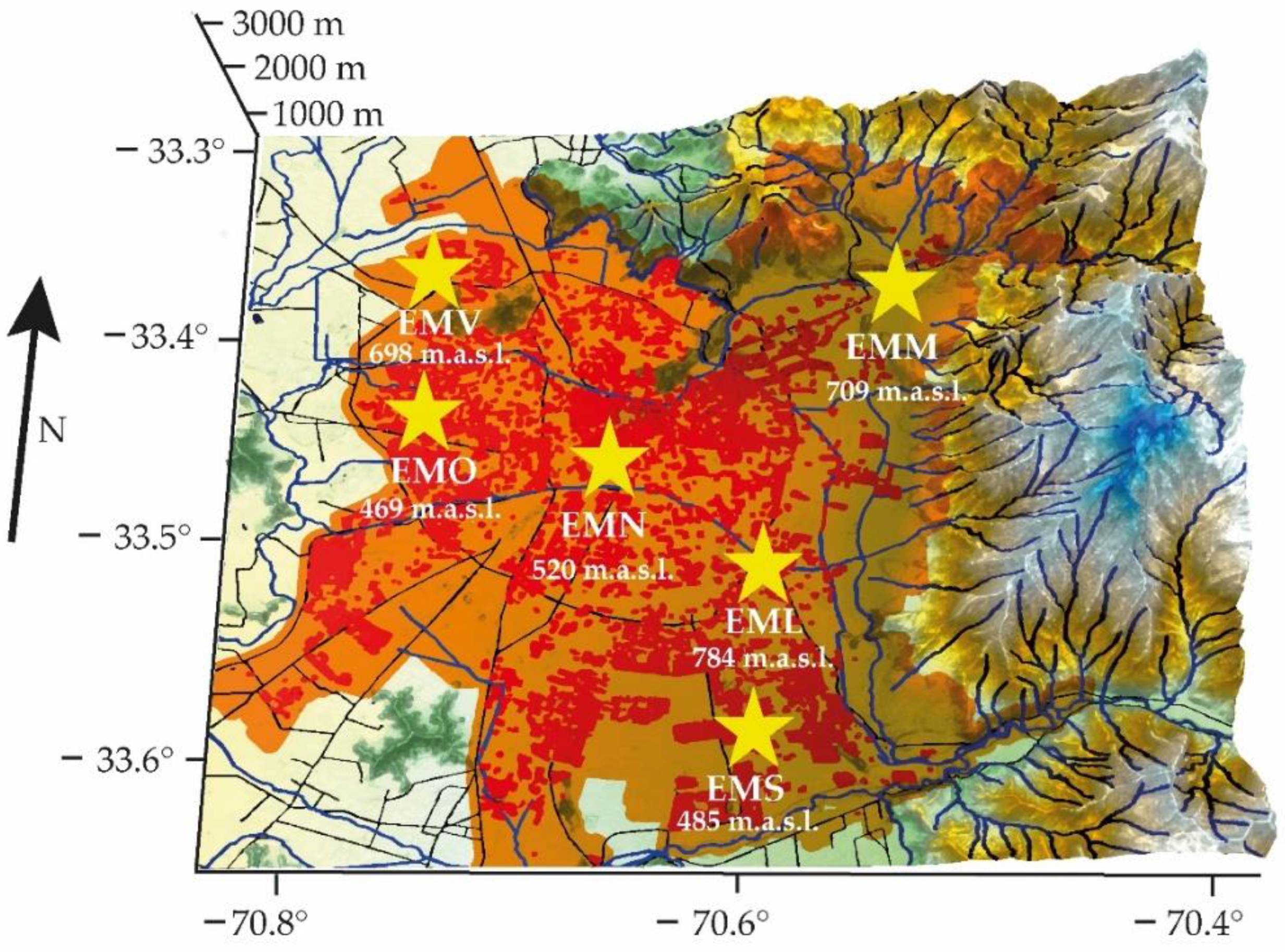
2.3. Study Area
3. Results
3.1. Meteorological Variables
3.2. Pollutants
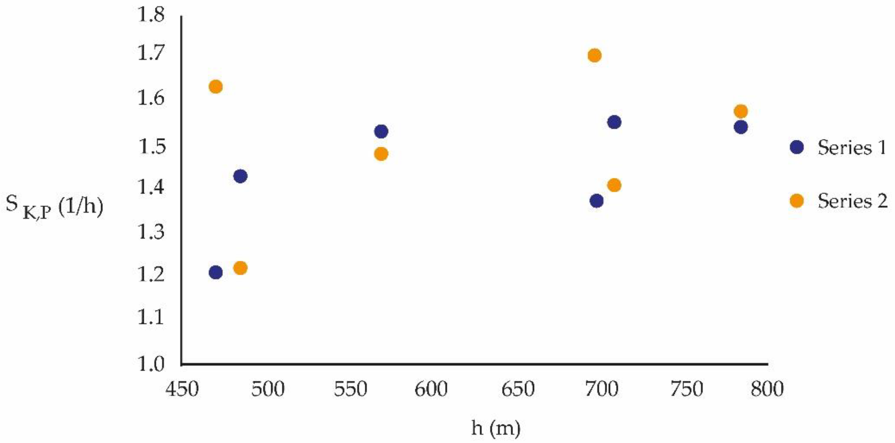
3.3. Relationship between SK,MV and SK,P
4. Discussion
5. Conclusions
Author Contributions
Funding
Institutional Review Board Statement
Informed Consent Statement
Data Availability Statement
Acknowledgments
Conflicts of Interest
Appendix A

| PM10 | PM2.5 | CO | T | HR | WV | ||
|---|---|---|---|---|---|---|---|
| EML | 2010–2013 | ||||||
| H | 0.967 | 0.973 | 0.959 | 0.989 | 0.991 | 0.976 | |
| D | 1.033 | 1.027 | 1.041 | 1.011 | 1.009 | 1.024 | |
| 2017–2020 | |||||||
| H | 0.922 | 0.963 | 0.933 | 0.915 | 0.942 | 0.975 | |
| D | 1.078 | 1.037 | 1.067 | 1.085 | 1.058 | 1.025 | |
| EMM | 2010–2013 | ||||||
| H | 0.972 | 0.977 | 0.981 | 0.991 | 0.990 | 0.980 | |
| D | 1.028 | 1.023 | 1.019 | 1.009 | 1.010 | 1.02 | |
| 2017–2020 | |||||||
| H | 0.906 | 0.983 | 0.933 | 0.917 | 0.941 | 0.976 | |
| D | 1.094 | 1.017 | 1.067 | 1.083 | 1.059 | 1.024 | |
| EMN | 2010–2013 | ||||||
| H | 0.972 | 0.974 | 0.953 | 0.989 | 0.991 | 0.968 | |
| D | 1.028 | 1.026 | 1.047 | 1.011 | 1.009 | 1.032 | |
| 2017–2020 | |||||||
| H | 0.929 | 0.960 | 0.933 | 0.916 | 0.942 | 0.973 | |
| D | 1.071 | 1.04 | 1.067 | 1.084 | 1.058 | 1.027 | |
| EMO | 2010–2013 | ||||||
| H | 0.965 | 0.955 | 0.937 | 0.992 | 0.989 | 0.968 | |
| D | 1.035 | 1.045 | 1.063 | 1.008 | 1.011 | 1.032 | |
| 2017–2020 | |||||||
| H | 0.936 | 0.925 | 0.933 | 0.919 | 0.942 | 0.974 | |
| D | 1.064 | 1.075 | 1.067 | 1.081 | 1.058 | 1.026 | |
| EMS | 2010–2013 | ||||||
| H | 0.969 | 0.973 | 0.953 | 0.990 | 0.992 | 0.957 | |
| D | 1.031 | 1.027 | 1.047 | 1.010 | 1.008 | 1.043 | |
| 2017–2020 | |||||||
| H | 0.921 | 0.975 | 0.933 | 0.915 | 0.942 | 0.976 | |
| D | 1.079 | 1.025 | 1.067 | 1.085 | 1.058 | 1.024 | |
| EMV | 2010–2013 | ||||||
| H | 0.967 | 0.970 | 0.952 | 0.989 | 0.989 | 0.956 | |
| D | 1.033 | 1.03 | 1.048 | 1.011 | 1.011 | 1.044 | |
| 2017–2020 | |||||||
| H | 0.931 | 0.966 | 0.933 | 0.919 | 0.942 | 0.975 | |
| D | 1.069 | 1.034 | 1.067 | 1.081 | 1.058 | 1.025 | |
| Stations | EML | EMM | EMV | EMN | EMS | EMO |
|---|---|---|---|---|---|---|
| Periods | H; LZ | H; LZ | H; LZ | H; LZ | H; LZ | H; LZ |
| 2010–2013 | 0.976; 0.320 | 0.980; 0.558 | 0.956; 0.325 | 0.968; 0.286 | 0.957; 0.293 | 0.968; 0.538 |
| 2017–2020 | 0.975 (=); 0.551 (>) | 0.976 (=); 0.557 (=) | 0.975 (>); 0.544 (>) | 0.973 (>);0.539 (>) | 0.976 (>); 0.556 (>) | 0.974 (>); 0.537 (=) |
References
- Cox, D.T.C.; Gaston, K.J. Human–nature interactions and the consequences and drivers of provisioning wildlife. Phil. Trans. R. Soc. B 2018, 373, 20170092. [Google Scholar] [CrossRef] [PubMed]
- Holling, C.S. Resilience and Stability of Ecological Systems. Annu. Rev. Ecol. Syst. 1973, 4, 1–23. [Google Scholar] [CrossRef]
- Morrison, H.; Gijs de Boer, G.; Feingold, G.; Feingold, G.; Harrington, J.; Shupe, M.D.; Sulia, K. Resilience of persistent Arctic mixed-phase clouds. Nat. Geosci. 2012, 5, 11–17. [Google Scholar] [CrossRef]
- González, J.E.; Ramamurthy, P.; Bornstein, R.D.; Chen, F.; Bou-Zeid, E.R.; Ghandehari, M.; Luvall, J.; Mitra, C.; Niyogi, D. Urban climate and resiliency: A synthesis report of state of the art and future research directions. Urban Clim. 2021, 38, 100858. [Google Scholar] [CrossRef]
- Figueiredo, L.; Honiden, T.; Schumann, A. Indicators for Resilient Cities. In OECD Regional Development Working Papers; No. 2018/02; OECD Publishing: Paris, France, 2018. [Google Scholar] [CrossRef]
- Travaglini, S.; Noble, J.; Ross, P.G.; Dharan, C.K.H. Mycology Matrix Composites. In Proceedings of the American Society for Composites—Twenty-Eighth Technical Conference (Annual Technical Conference 28th, American Society for Composites), State College, PA, USA, 9–11 September 2013; Curran Associates, Inc., Red Hook: New York, NY, USA, 2013; pp. 517–535, ISBN 9781629931432. (British Library Conference Proceedings). [Google Scholar]
- Mauree, D.; Coccolo, S.; Deschamps, L.; Loesch, P.; Becquelin, P.; Scartezzini, J.L. Mobile Urban Micrometeorological Monitoring (MUMiM). J. Phys. Conf. Ser. 2019, 1343, 012014. [Google Scholar] [CrossRef]
- Foken, T. Micrometeorology; Springer: Berlin/Heidelberg, Germany, 2008. [Google Scholar]
- Stull, R.B. Introduction to Boundary Layer Meteorology; Kluwer Academic: Alphen aan den Rijn, The Netherlands, 1988; 666p. [Google Scholar]
- Klausner, Z.; Ben-Efraim, M.; Arav, Y.; Tas, E.; Fattal, E. The Micrometeorology of the Haifa Bay Area and Mount Carmel during the summer. Atmosphere 2021, 12, 354. [Google Scholar] [CrossRef]
- Garratt, J.R.; Pearman, G.I. Retrospective Analysis of Micrometeorological Observations Above an Australian Wheat Crop. Bound.-Layer Meteorol. 2020, 177, 613–641. [Google Scholar] [CrossRef]
- Landsberg, H.E. Micrometeorological temperature differentiation through urbanization. In Urban Ctimates, Technical Note, No. 108; World Meteorologicai Organization: Geneva, Switzerland, 1970; pp. 129–136. [Google Scholar]
- Landsberg, H.E.; Maisel, T.N. Micrometeorological observations in an area of urban growth. Bound.-Layer Meteorol. 1972, 2, 365–370. [Google Scholar] [CrossRef]
- Bénard, H. Les tourbillons cellulaires dans une nappe liquide propageant de la chaleur par convection en régime permanent. Ann. Chim. Phys. 1901, 23, 62–164. [Google Scholar] [CrossRef]
- Brillouin, L. Science and Information Theory, 2nd ed.; Academic Press: New York, NY, USA, 1962; 304p. [Google Scholar]
- Haddad, W. Thermodynamics: The Unique Universal Science. Entropy 2017, 19, 621. [Google Scholar] [CrossRef]
- Prigogine, I. Introduction to Thermodynamics of Irreversible Processes; Thomas, C.C., Ed.; ACS Publications: Springfield, IL, USA, 1955; 115p. [Google Scholar]
- Sinai, Y.G. On the concept of entropy of a dynamical system. Dokl. Akad. Nauk SSSR 1959, 124, 768–777. [Google Scholar]
- Dewar, R.C. Maximum entropy production and the fluctuation theorem. J. Phys. A Math. Gen. 2005, 38, 1371–1381. [Google Scholar] [CrossRef]
- Bengtsson, I.; Życzkowski, K. Geometry of Quantum States: An Introduction to Quantum Entanglement, 301, 2nd ed.; Cambridge University Press: Cambridge, UK, 2017. [Google Scholar]
- Parker, D. The H-Theorem, Molecular Disorder and Probability: Perspectives from Boltzmann’s Lectures on Gas Theory PhilSci Arch 2009, OAI–Open Archives Initiative. Available online: http://philsci-archive.pitt.edu/id/eprint/5005 (accessed on 26 November 2020).
- Shannon, C. A mathematical theory of communication. Bell Syst. Tech. 1948, 27, 379–423. [Google Scholar] [CrossRef]
- Sprott, J.C. Chaos and Time-Series Analysis; Oxford University Press: Oxford, UK, 2003; 528p. [Google Scholar]
- Ruelle, D.P. Extending the definition of entropy to nonequilibrium steady states. Proc. Natl. Acad. Sci. USA 2003, 100, 3054–3058. [Google Scholar] [CrossRef]
- Lin, Y.; Lin, C.; Wang, D. Understanding Atmospheric Behaviour in Terms of Entropy: A Review of Applications of the Second Law of Thermodynamics to Meteorology. Entropy 2011, 13, 211–240. [Google Scholar] [CrossRef]
- Farmer, J.D. Chaotic attractors of an infinite dimensional dynamical system. Physica D 1982, 4, 366–393. [Google Scholar] [CrossRef]
- Farmer, J.D.; Otto, E.; Yorke, J.A. The dimension of chaotic attractors. Physica D 1983, 7, 153–180. [Google Scholar] [CrossRef]
- Kolmogorov, A.N. On Entropy per unit Time as a Metric Invariant of Automorphisms. Dokl. Akad. Nauk SSSR 1959, 124, 754–755. [Google Scholar]
- Martínez, J.A.; Vinagre, F.A. La Entropía de Kolmogorov; su Sentido Físico y su Aplicación al Estudio de Lechos Fluidizados 2D. Departamento de Química Analítica e Ingeniería Química, Universidad de Alcalá, Alcalá de Henares, Madrid, España. Available online: https://www.academia.edu/247937219/07/2019 (accessed on 20 September 2020).
- Pacheco, P.; Mera, E. Relations between Urban Entropies, Geographical Configurations, Habitability and Sustainability. Atmosphere 2022, 13, 1639. [Google Scholar] [CrossRef]
- Shaw, R. Strange attractors, chaotic behavior and information flow. Z. Naturforsch. A 1981, 36, 80–112. [Google Scholar] [CrossRef]
- Cohen, A.; Procaccia, I. Computing the Kolmogorov entropy from time signals of dissipative and conservative dynamical systems. Phys. Rev. A Gen. Phys. 1985, 31, 1872–1882. [Google Scholar] [CrossRef] [PubMed]
- MMA, Sistema de Información Nacional de Calidad del Aire (Ministerio del Medioambiente de Chile). Available online: https://sinca.mma.gob.cl/index.php (accessed on 23 April 2022).
- Takens, F. Detecting Strange Attractors in Turbulence. In Dynamical Systems and Turbulence, Warwick 1980; Rand, D., Young, L.S., Eds.; Springer: Berlin, Germany, 1981; pp. 366–381. [Google Scholar] [CrossRef]
- Eckmann, J.P.; Oliffson, S.; Kamphorst, S.; Ruelle, D.; Ciliberto, C. Lyapunov exponents from time series. Phys. Rev. A 1986, 34, 4971–4979. [Google Scholar] [CrossRef] [PubMed]
- Grassberger, P.; Procaccia, L. Characterization of strange attractors. Phys. Rev. Lett. 1983, 50, 346–349. [Google Scholar] [CrossRef]
- Wolf, A.; Swift, J.B.; Swinney, H.L.; Vastano, J.A. Determining Lyapunov exponents from a time series. Physica D 1985, 16, 285–317. [Google Scholar] [CrossRef]
- Gao, J.; Cao, Y.; Hu, J. Multiscale Analysis of Complex Time Series; Wiley and Sons Interscience: Hoboken, NJ, USA, 2007; 368p. [Google Scholar]
- Chelani, A.; Devotta, S. Nonlinear analysis and prediction of coarse particulate matter concentration in ambient air. J. Air Waste Manag. Asoc. 2006, 56, 78–84. [Google Scholar] [CrossRef]
- Horna Mercedes, J.; Dionicio Vereau, J.; Martínez Zocón, R.; Zavaleta Quipuscoa, A.; Brenis Delgado, Y. Dinámica Simbólica y Algunas Aplicaciones. Sel. Matemáticas 2016, 3, 101–106. [Google Scholar] [CrossRef]
- Kantz, H.; Schreiber, T. Nonlinear Time Series Analysis, 2nd ed.; Cambridge University Press: Cambridge, UK, 2004; 387p. [Google Scholar]
- Sivakumar, B.; Wallender, W.; Horwath, W.; Mitchell, J. Nonlinear deterministic analysis of air pollution dynamics in a rural and agricultural setting. Adv. Complex Syst. 2007, 10, 581–597. [Google Scholar] [CrossRef]
- Lee, C.K.; Lin, S.C. Chaos in air pollutant concentration (APC) time series. Aerosol Air Qual. Res. 2008, 8, 381–391. [Google Scholar] [CrossRef]
- Kumar, U.; Prakash, A.; Jain, V.K. Characterization of chaos in air pollutants: A Volterra-Wiener-Korenberg series and numerical titration approach. Atmos. Environ. 2008, 42, 1537–1551. [Google Scholar] [CrossRef]
- Fraser, A.M.; Swinney, H.L. Independent coordinates for strange attractors from mutual information. Phys. Rev. A 1986, 33, 1134–1140. [Google Scholar] [CrossRef]
- Malyutina, E.I.; Shiryaev, V.I. Time Series Forecasting Using Nonlinear Dynamic Methods and Identification of Deterministic Chaos. Procedia Comput. Sci. 2014, 31, 1022–1103. [Google Scholar] [CrossRef]
- Salini, G.; Pérez, P. A study of the dynamic behavior of fine particulate matter in Santiago, Chile. Aerosol Air Qual. Res. 2015, 15, 154–165. [Google Scholar] [CrossRef]
- Pacheco, P.R.; Parodi, M.C.; Mera, E.M.; Salini, G.A. Variables meteorológicas y niveles de concentración de material particulado de 10 μm en Andacollo, Chile: Un estudio de dispersión y entropías. Inf. Tecnológica 2020, 31, 171–182. [Google Scholar] [CrossRef]
- Pacheco, P.R.; Salini, G.A.; Mera, E.M. Entropía y Neguentropía: Una aproximación al proceso de difusión de contaminantes y su sostenibilidad. Rev. Int. Contam. Ambient. 2021, 37, 167–185. [Google Scholar] [CrossRef]
- Salini, G.A.; Pacheco, P.R.; Mera, E.; Parodi, M.C. Probable Relationship between COVID-19, Pollutants and Meteorology: A Case Study at Santiago, Chile. Aerosol Air Qual. Res. 2021, 21, 200434. [Google Scholar] [CrossRef]
- Pacheco, P.; Mera, E.; Salini, G. Urban Densification Effect on Micrometeorology in Santiago, Chile: A Comparative Study Based on Chaos Theory. Sustainability 2022, 14, 2845. [Google Scholar] [CrossRef]
- Norazian, M.N.; Shruki, Y.A.; Azam, R.M.; Mustafa Al Bakri, A.M. Estimation of missing values in air pollution data using single imputation techniques. ScienceAsia 2008, 34, 341–345. [Google Scholar] [CrossRef]
- Junninen, H.; Niska, H.; Tuppurainen, K.; Ruuskanen, J.; Kolehmainen, M. Methods for imputation of missing values in air quality data sets. Atmos. Environ. 2004, 38, 2895–2907. [Google Scholar] [CrossRef]
- Asa, E.; Saafi, M.; Membah, J.; Billa, A. Comparison of linear and nonlinear Kriging methods for characterization and interpolation of soil data. J. Comput. Civil Eng. 2012, 26, 11–18. [Google Scholar] [CrossRef]
- Emery, X. Simple and ordinary multigaussian Kriging for estimating recoverable reserves. Math. Geol. 2005, 37, 295–319. [Google Scholar] [CrossRef]
- Kyriakidis, P.; Journel, A. Geostatistical space-time models: A review. Math. Geol. 1999, 6, 651–684. [Google Scholar] [CrossRef]
- Rutland, J.; Garreaud, R. Meteorological air pollution for Santiago, Chile: Towards an objective episode forecasting. Environ. Monit. Assess. 1995, 34, 223–244. [Google Scholar] [CrossRef] [PubMed]
- Rubio, M.A.; Fuenzalida, I.; Salinas, E.; Lissi, E.; Kurtenbach, R.; Wiesen, P. Carbon monoxide and carbon dioxide concentrations in Santiago de Chile associated with traffic emissions. Environ. Monit. Assess. 2010, 162, 209–217. [Google Scholar] [CrossRef] [PubMed]
- Livert Aquino, F.; Gainza, X. Understanding Density in an Uneven City, Santiago de Chile:Implications for Social and Environmental Sustainability. Sustainability 2014, 6, 5876–5897. [Google Scholar] [CrossRef]
- Vicuña, M. Density and its Effects on the Spatial Transformation of the Contemporary City: Five Typologies to Understand Residential Densification in Santiago Metropolitan Area. Revista 180 2020, 45, 112–126. [Google Scholar] [CrossRef]
- Saaroni, H.; Baruch Ziv, B. Estimating the Urban Heat Island Contribution to Urban and Rural Air Temperature Differences over Complex Terrain: Application to an Arid City. J. Appl. Meteorol. Climatol. 2010, 49, 2159–2166. [Google Scholar] [CrossRef]
- Tursilowati, L.; Sumantyo, J.T.S.; Kuze, H.; Adiningsih, E.S. The integrated wrf/urban modeling system and its application to monitoring urban heat island in Jakarta, indonesia. J. Urban Environ. Eng. 2012, 6, 1–9. [Google Scholar] [CrossRef]
- Lee, S.H.; Kim, S.W.; Angevine, W.; Bianco, L.; McKeen, S.; Senff, C.; Trainer, M.; Tucker, S.; Zamora, R. Evaluation of urban surface parameterizations in the WRF model using measurements during the Texas air quality study 2006 field campaign. Atmos. Chem. Phys. 2011, 11, 2127–2143. [Google Scholar] [CrossRef]
- Chen, Y.-C.; Fröhlich, D.; Matzarakis, A.; Ping Lin, T. Urban Roughness Estimation Based on Digital Building Models for Urban Wind and Thermal Condition Estimation—Application of the SkyHelios Model. Atmosphere 2017, 8, 247. [Google Scholar] [CrossRef]
- Vergara, J.E. Verticalización. La Edificación en Altura en la Región Metropolitana de Santiago (1990–2014), Revista INVI 2017, 32, 9–49. [Google Scholar]
- Craig, S.; Grinham, J. Breathing walls: The design of porous materials for heat exchange and decentralized ventilation. Energy Build. 2017, 149, 246–259. [Google Scholar] [CrossRef]


| Station | m.a.s.l. (m) | Series 1 | Series 2 |
|---|---|---|---|
| 2010–2013 | 2017–2020 | ||
| SK,MV (1/h) | SK,MV (1/h) | ||
| EML | 784 | 1.334 | 1.284 |
| EMM | 709 | 1.452 | 1.205 |
| EMO | 469 | 1.197 | 0.993 |
| EMS | 698 | 1.289 | 1.250 |
| EMV | 485 | 1.202 | 0.994 |
| EMN | 570 | 1.262 | 1.145 |
| Station | m.a.s.l. (m) | Series 1 | Series 2 |
|---|---|---|---|
| 2010–2013 | 2017–2020 | ||
| SK,P (1/h) | SK,P (1/h) | ||
| EML | 784 | 1.542 | 1.577 |
| EMM | 709 | 1.550 | 1.406 |
| EMO | 469 | 1.210 | 1.630 |
| EMS | 698 | 1.377 | 1.702 |
| EMV | 485 | 1.431 | 1.220 |
| EMN | 570 | 1.531 | 1.479 |
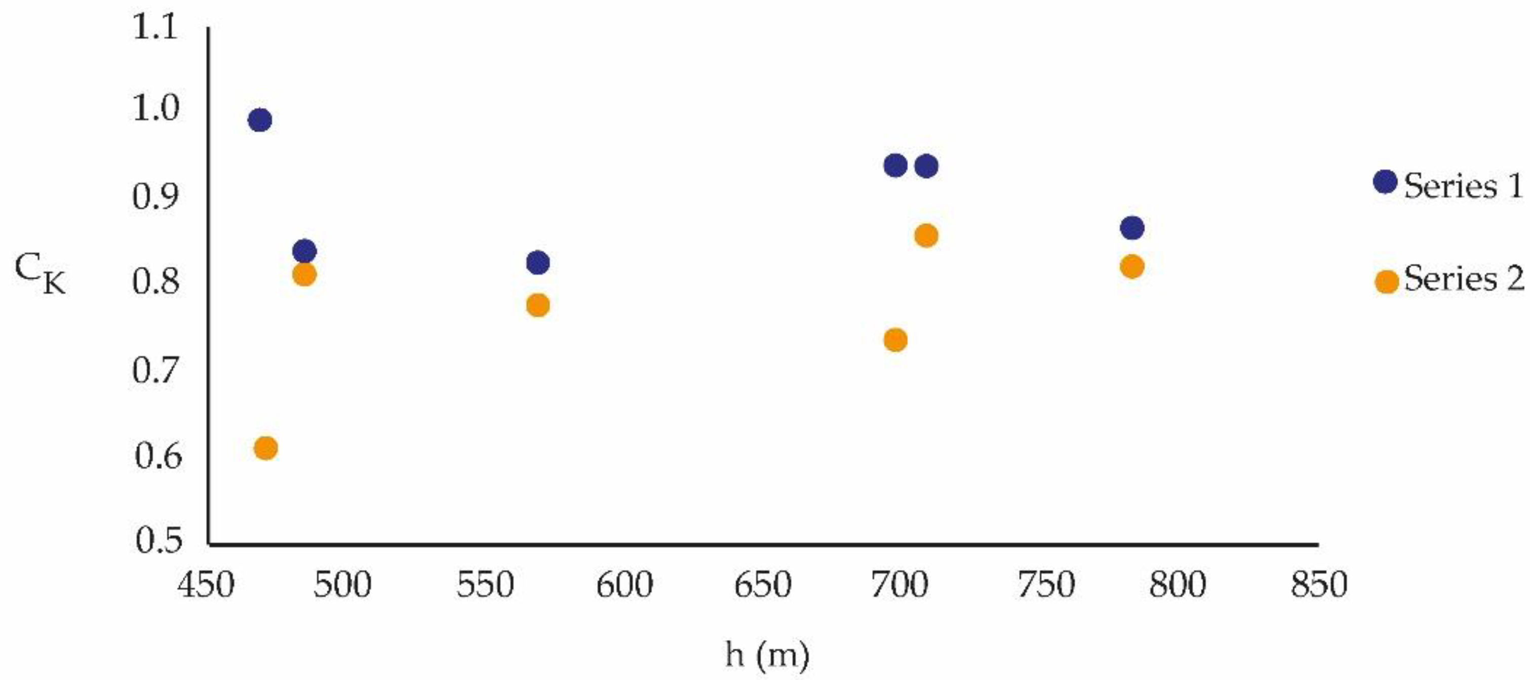
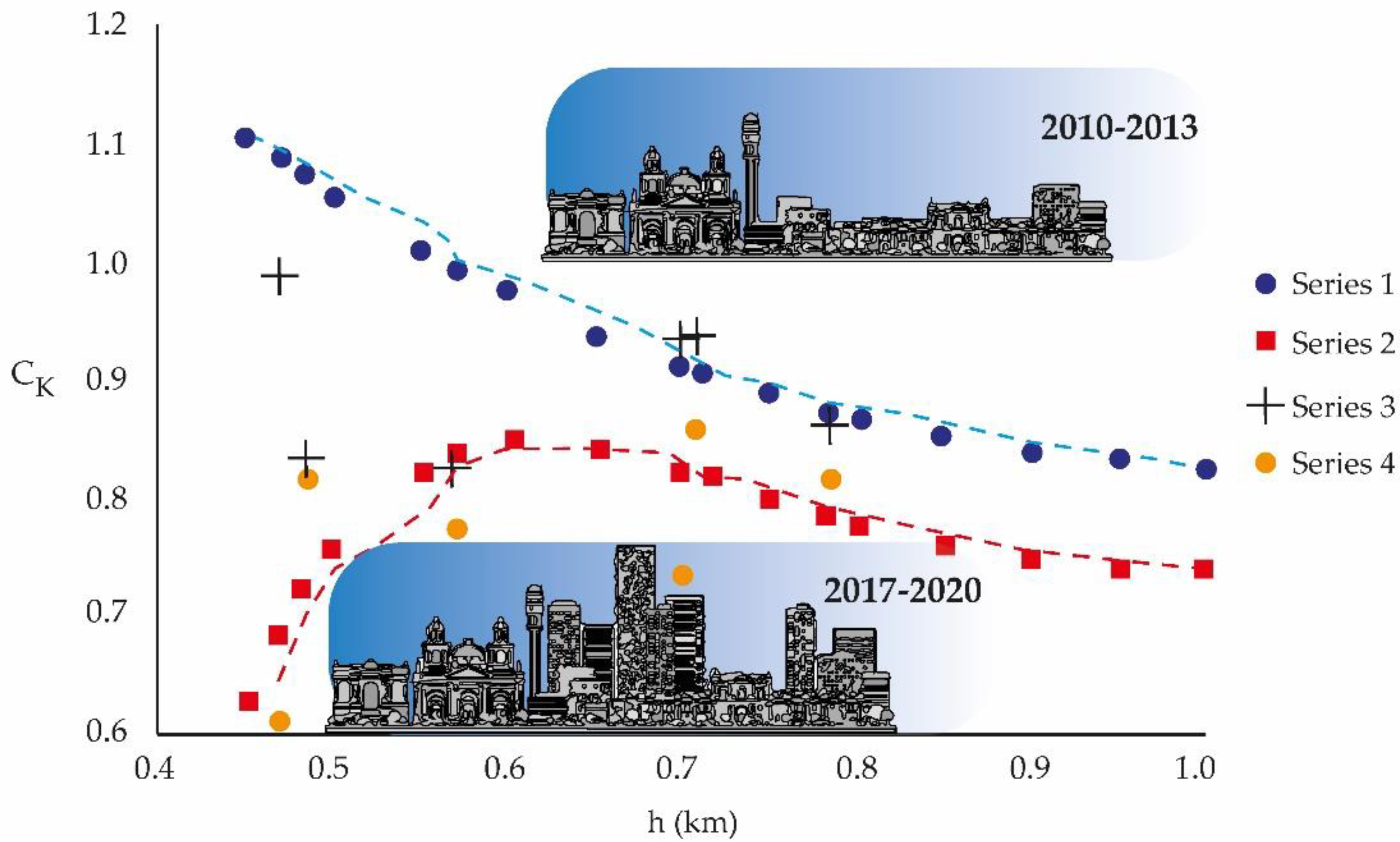
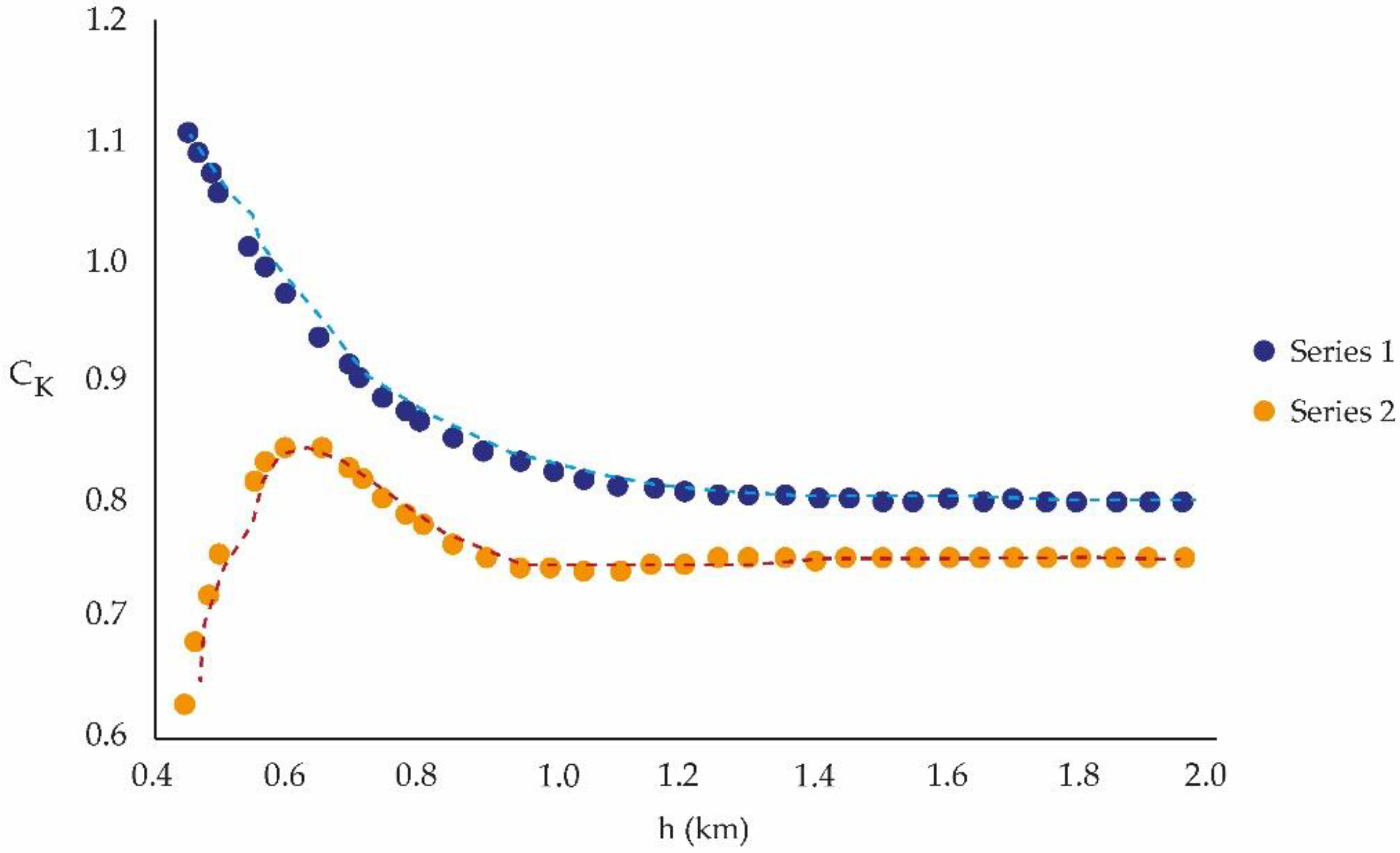
| h (m.a.s.l.) | 2010–2013 | 2017–2020 | % Variation |
|---|---|---|---|
| CK1 (Series 1) | CK2 (Series 2) | ||
| 784 (EML) | 0.865 | 0.814 | 6 |
| 709 (EMM) | 0.937 | 0.857 | 7 |
| 485 (EMV) | 0.834 | 0.815 | 3 |
| 570 (EMN) | 0.824 | 0.774 | 7 |
| 698 (EMS) | 0.936 | 0.734 | 22 |
| 469 (EMO) | 0.989 | 0.609 | 38 |
Disclaimer/Publisher’s Note: The statements, opinions and data contained in all publications are solely those of the individual author(s) and contributor(s) and not of MDPI and/or the editor(s). MDPI and/or the editor(s) disclaim responsibility for any injury to people or property resulting from any ideas, methods, instructions or products referred to in the content. |
© 2023 by the authors. Licensee MDPI, Basel, Switzerland. This article is an open access article distributed under the terms and conditions of the Creative Commons Attribution (CC BY) license (https://creativecommons.org/licenses/by/4.0/).
Share and Cite
Pacheco, P.; Mera, E.; Fuentes, V.; Parodi, C. Initial Conditions and Resilience in the Atmospheric Boundary Layer of an Urban Basin. Atmosphere 2023, 14, 357. https://doi.org/10.3390/atmos14020357
Pacheco P, Mera E, Fuentes V, Parodi C. Initial Conditions and Resilience in the Atmospheric Boundary Layer of an Urban Basin. Atmosphere. 2023; 14(2):357. https://doi.org/10.3390/atmos14020357
Chicago/Turabian StylePacheco, Patricio, Eduardo Mera, Voltaire Fuentes, and Carolina Parodi. 2023. "Initial Conditions and Resilience in the Atmospheric Boundary Layer of an Urban Basin" Atmosphere 14, no. 2: 357. https://doi.org/10.3390/atmos14020357