Assessing the Spatial Distribution of NO₂ and Influencing Factors in Urban Areas—Passive Sampling in a Citizen Science Project in Berlin, Germany

Abstract

Nitrogen dioxide (NO₂) is a major air pollutant with diverse impacts on human health and the environment. In urban areas, road traffic is the main emission source for NO₂. In Berlin, Germany, a network of measurement stations is operated by the state, fulfilling the monitoring requirements set by the European Union. To get a more detailed overview of the spatial distribution of NO₂ concentrations in Berlin, a citizen science project allowed for collection of additional data and an increase in the number of sampling sites. Passive samplers (modified Palmes tubes) were distributed to participants to collect NO₂ at a site of their choice. When returned, the samplers were analyzed based on the Griess–Ilosvay reaction and spectrophotometric detection. The results confirmed a seasonal trend of higher NO₂ concentrations in winter and lower concentrations during the summer period. Furthermore, the spatially and monthly averaged NO₂ concentrations observed in the study period from March 2019 to October 2020 were in good agreement with the average urban background concentration. At small spatial scales, a tendency of decreasing NO₂ concentrations with increasing distance from roads was observed. Overall, this study shows the added benefit of extensive low-cost measurements of NO₂ concentrations across urban environments in a citizen science project to complement stationary air pollution monitoring networks.

1. Introduction

Nitrogen dioxide (NO₂) is a major air pollutant with adverse health effects, in particular, respiratory diseases such as asthma. Moreover, it acts as a precursor of ozone and particulate matter [1].

Combustion processes, especially due to road traffic, are the major contributors to the concentration of NO₂ in urban areas [2]. In the European Union and its member states, a limit value for annual NO₂ concentrations of 40 µg/m³ has been implemented [3]. In Germany, the monitoring of air pollutants, including NO_2, is statutory and officially carried out by the federal states. In 2019, the air pollution monitoring network of Berlin (Berliner Luftgütemessnetz, BLUME) consisted of 16 stationary and continuously monitoring sites (18 monitoring sites in 2020) with nitrogen monoxide (NO) and NO₂ measurements based on chemiluminescence [4,5]. BLUME is complemented by the RUBIS measurement network (for soot, benzene, and NO₂), providing 36 (in 2019; 42 in 2020) additional measuring sites at main roads using passive sampling for two-week averaged NO₂ concentrations [4,5]. Some of the reasons for the relatively large number of monitoring sites in Berlin are past exceedances of limit values (e.g., exceedance of the annual NO₂ limit value at one BLUME and several RUBIS sites in 2019), the evaluation of air quality management measures, and the validation of modeled, spatially resolved NO₂ values [4,5].

Multiple local emission sources in urban areas show a complex spatial and temporal pattern [6,7,8]. Thus, urban NO₂ concentrations are highly variable, and stationary monitoring stations may not be representative for a larger area [9,10]. Hence, it is of particular importance to identify the spatial variability of NO₂ concentrations in urban areas and to understand the main drivers and influencing factors (e.g., traffic volume, roadside structures, and meteorological conditions).

Citizen science initiatives with a focus on air quality enjoy increasing popularity in recent years. The involvement of citizen scientists is beneficial to allowing to gather additional data and to significantly increase the number of measurements with relatively low effort. In recent years, several citizen science projects have been carried out on air pollution in general, e.g., in urban areas in California and Colorado in the United States, in the Republic of Korea, and in Kenya [11,12,13,14], and specifically on urban NO₂ concentrations, e.g., in Italy [15]. An impressive example of a large citizen science project on air pollution is a NO₂ distribution survey over Flanders (Belgium) in 2018. About 20,000 passive samplers were distributed to interested citizen scientists and simultaneously deployed by the participants over a four-week sampling period in 2018. The outcome of this campaign not only presented unique information about NO₂ concentration distribution and exposure of the population, but also complemented measurements taken by official air quality monitoring networks and supported the improvement of air quality models [16,17]. It should be noted that most citizen science data do not meet the criteria for checking annual limit values; however, efforts have been made to combine statistical modeling and citizen science data to estimate annual average concentrations from multi-week sampling campaigns [18].

In Germany, several citizen science campaigns were initiated by Environmental Action Germany (DUH) to measure the air quality, focusing on NO₂. For example, during campaigns in 2018 and 2019, passive samplers were sent to selected persons upon request. The sampling time was generally four weeks at a specific site, but the sampling times were not synchronized. Collection with diffusive passive samplers and spectrophotometric analysis of NO₂ took place in cities without official measurement sites, but also at sites where high NO₂ concentrations would harm vulnerable people, i.e., close to kindergartens, schools, hospitals, and nursing homes [19]. The main conclusion drawn from the results is that the annual limit value for NO₂ is probably exceeded everywhere at roadsides at high traffic volumes [20]. To extend the measurement network of NO₂ within urban areas, a citizen science project was also carried out in Munich, Germany, in autumn 2016. Passive sampling was employed at 50 sites in parallel all over the city for a sampling period of one to two months. Sampling sites included main roads, areas with low traffic volume, backyards of town houses, and green areas within Munich. The highest NO₂ concentrations were observed at roadsides, with a considerable number of values above 40 µg/m³. With increasing distance from main roads, NO₂ concentrations decreased considerably [21].

The results of the past 30 years of NO₂ monitoring in Berlin have shown, almost consistently, three levels of annual average NO₂ concentrations: 40–60 µg/m³ for sites at main roads, 20–40 µg/m³ in the urban background, and below 20 µg/m³ at suburban sites. In previous years, exceedances of annual NO₂ limit values (40 µg/m³) occurred at several roadside stations, but exceedances were not observed in 2020. In the past 10 years, several measuring campaigns by students of Technische Universität Berlin (TUB) were carried out, as well as a project on ambient NO₂ measurements supported by the regional Berlin broadcaster Rundfunk Berlin-Brandenburg (RBB).

Here, we present the main results of a citizen science project coordinated by the Environmental Chemistry and Air Research group at TUB, called the BerlinAir NO₂-Atlas, aiming to create a spatially comprehensive data set of urban NO₂ concentrations in Berlin [22]. We will provide the methodological details of the NO₂ sampling and analysis approach and illustrate the results obtained in the context of this citizen science project. The main research questions focused on the spatial distribution of NO₂ in Berlin and the comparison of the citizen science data with data from the Berlin air pollution monitoring network, BLUME.

2. Materials and Methods

Passive sampling of NO₂ was conducted as part of a citizen science project with sampling campaigns in 2019 and 2020. Passive sampling is simple to use and represents a low-cost method that can be installed without any power supply. A total of 1268 samples were collected and analyzed over the course of the citizen science project. During two intensive sampling periods in summer 2019 and in winter 2019/2020, 264 and 496 samples were collected and analyzed, respectively. The other samples were collected outside of these periods. In the following, the standard procedures for preparation of the passive samplers, NO₂ sampling and analysis, and data evaluation are described. For passive sampling of NO₂, modified Palmes tubes were used in this study [23,24]. The chemical analysis was based on the Griess–Ilosvay reaction and spectrophotometric detection. The quantification of NO₂ concentrations was based on Fick’s Law of diffusion [23,25]. A review of applications and limitations of passive sampling for the measurement of nitrogen dioxide in ambient air can be found in the literature [26,27].

2.1. Construction and Preparation of Passive Samplers

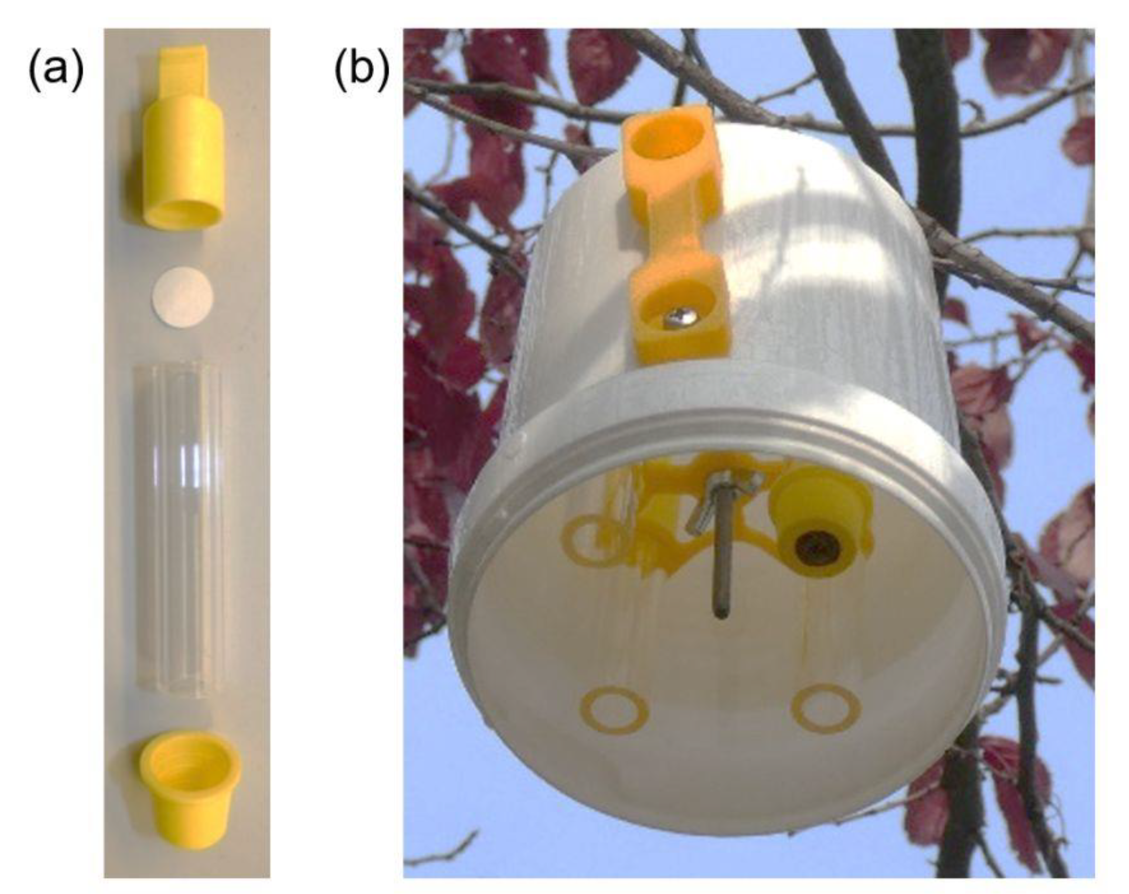
Tube-type passive samplers like those described by Palmes et al. (1976) [23] were built, using a polymethacrylate tube of 7.0 cm length and 1.0 cm inner diameter. Two polyethylene (PE) caps (protective caps for pipes GPN-250, Pöppelmann, Lohne, Germany) served to hold cotton pads (Rotilab 100% cotton linters, Carl Roth, Karlsruhe, Germany) of 13.0 mm diameter and 0.7 mm thickness for NO₂ absorption on one end of the tube, and to close the passive sampler on the other end during transportation and storage (cf. Figure 1a). Rather than using stainless steel grids as in the original Palmes tubes, cotton pads were preferred, because the absorbing solution is more evenly distributed across the surface. Moreover, the risk of contamination is reduced with single-use cotton pads compared with stainless steel grids that have to be cleaned after each sampling period.

In a number of previous investigations conducted at our department, it was confirmed that the sampling rate and analytical specifications between the original Palmes tubes and the modified ones do not show significant differences. The precision of parallel measurements is typically better than 15%. Moreover, good agreement between side-by-side chemiluminescence measurements and passive sampling using the modified tubes has been shown in a previous study, and systematic deviations have not been observed. The overall measurement uncertainty was always below 25%. The detection limit (LOD) for atmospheric NO₂ depends on sampling duration, standard deviation of blank values, and the detection limit of the analytical procedure for determination of nitrite formed (see below). Using 14 days’ sampling, the LOD is in the range 6–10 µg/m³.

To prepare the passive samplers for on-site sampling, a volume of 20 µL of 20% triethanolamine (TEA) solution was pipetted onto the single cotton pad placed in one of the PE caps. The polymethacrylate tube was pressed thoroughly into the cap, so that the pad was fixed at the bottom of the cap. The closure cap was mounted on top of the tube. For each measurement site, four passive sampler tubes were placed in a common holder, a small plastic bucket with a purpose-made inlay to fix the four sampling tubes properly (cf. Figure 1b). The openings of the sampling tubes were levelled with the downward opening of the bucket to minimize possible wind effects [28].

In the citizen science project, the passive samplers were either picked up by the participants from the laboratory or (on request) sent to the participants by mail or courier along with instructions and a record sheet to be filled out during the sampling process.

2.2. NO₂ Sampling Procedure on Site

The citizen scientists decided themselves about the specific location of the measuring sites and sampled over a period of 14 days with an accepted range of +/− three days. The exposure time of two weeks facilitated an increase in the number of measuring points and hence the number of samples obtained. It is also a compromise between temporal resolution and required sensitivity of subsequent chemical analysis. Since only a few specifications were given regarding the measuring site parameters, the measurements were performed at diverse sites, including main streets, side roads, backyards, open spaces, and indoor environments.

The passive sampler was mounted on-site with cable ties. After installing the sampler, the closure caps of three of four sampling tubes were removed, and the start time of exposure was recorded. The fourth sampling tube remained closed and served as a field blank. At the end of the exposure time, the three open sampling tubes were closed by caps, and all four sampling tubes returned to the laboratory for analysis. The record sheet to be filled out by participants included the start and end times of the sampling period, the exact sampling location (address or GPS data), the height above the ground of the passive sampler, the distance to the road, and also additional information such as number of traffic lanes, local speed limits, type of road (main, side, residential), bus traffic, weather conditions, and other specifications about the location. The given information was used to categorize the sample results. An overview of sampling locations used during two intensive observation periods in summer 2019 and in winter 2019/2020 can be found in Tables S1 and S2 (Supplementary Materials) and in Figure 2 below.

2.3. Laboratory Evaluation of Formed Nitrite

In order to obtain average NO₂ concentrations of the two-week sampling periods, nitrite formed by reaction of NO₂ with TEA was photometrically determined in the laboratory. To extract the collected nitrite from the passive sampler, the PE cap containing the cotton pad with the TEA solution was cautiously removed from the sampling tube and placed on top of a purpose-made block with insets to warrant stable positioning. Deionized water in the amount of 2 mL was pipetted into the cap. For complete extraction of nitrite, the entire block was moved forward and backward horizontally for about 1 min. Exactly 1 mL of the extract was taken from the cap with a pipette and transferred into a small glass vial. For the Griess–Ilosvay reaction, 1 mL of sulfanilamide (SA) reagent solution and 100 µL of N-[naphthyl-(1)]-ethylendiamine-dihydrochloride (NED) reagent solution were successively added to form a pink-red azo dye with nitrite. After complete mixing, the reagent mixture was left for a minimum of 15 min for full color development. Eventually, a quartz cuvette of 1 cm path length was filled with the sample solution. Photometric measurement was conducted at a wavelength of λ = 540 nm wavelength against pure water as reference. A detailed description of the preparation of the reagent solutions can be found in Appendix A.

2.4. Calibration and Calculation of Results

A calibration curve for nitrite in the concentration range 0.1–5 mg/L was generated, using appropriate nitrite standard solutions to which SA and NED reagent solutions were added in a 10:10:1 ratio. After mixing and waiting for a minimum of 15 min, the absorbance was measured at a wavelength of λ = 540 nm against water as reference. The calibration curve was used for calculation of nitrite concentrations in the extracts of the passive samplers. The linear range of the calibration with a coefficient of determination R² = 0.99 was between 0.1 and 2 mg/L nitrite. Precision of repetitive measurements is typically below 3% RSD [24]. The LOD of the photometric method has been found to be 13 µg/L using a Specord 205 photometer (Analytik Jena, Jena, Germany) [24].

To check the consistency of the analytical procedure during the entire citizen science project, the slope of the calibration function was evaluated with each set of samplers. To this end, generally, only a single nitrite standard of 1 mg/L was employed. An absorbance value of 0.52 ± 10% (1 cm cuvette path length) was accepted to be a reasonable result. In case of higher deviations, the entire procedure (including the preparation of reagent solutions) was re-evaluated.

Nitrite concentrations in the extract of passive samplers, c_{nitrite,sample} (in mg/L), were calculated according to Equation (1),

$${\mathrm{c}}_{\mathrm{nitrite}, \mathrm{sample}}=\frac{{\mathrm{c}}_{\mathrm{nitrite}, \mathrm{ref}}}{{\mathrm{A}}_{\mathrm{ref}}}\times { \mathrm{A}}_{\mathrm{sample}}$$

(1)

with c_nitrite,ref, being the nitrite concentration in the reference solution in mg/L, A_ref, the absorbance of the reference solution (dimensionless), and A_sample, the absorbance of the sample solution (dimensionless).

Since TEA serves as an ideal sink for NO₂, and since the conversion factor of NO₂ to nitrite is unity, i.e., the mass of nitrite on the filter corresponds to the mass of NO₂ [29], the mass of NO₂ collected was calculated according to Equation (2), considering the extraction volume of 2 mL,

$${\mathrm{m}}_{{\mathrm{NO}}_{2,\mathrm{sample}}}={\mathrm{m}}_{\mathrm{nitrite},\mathrm{sample}}={\mathrm{c}}_{\mathrm{nitrite},\mathrm{sample}}\times {\mathrm{V}}_{\mathrm{extraction}}$$

(2)

With m_NO2,sample, the mass of NO₂ collected in sample (in mg), m_{nitrite,sample}, mass of nitrite in sample extract (in mg), and V_extraction, the extraction volume (in L).

To calculate the average NO₂ concentration in the ambient air during the sampling period from the collected mass of NO₂, Fick’s law of diffusion was applied. With the mass of NO₂ collected, m_NO2,sample in mg from Equation (2), the given sampler geometry, i.e., the length of the sampling tube L_tube = 7 cm and the cross-sectional area of the sampling tube A_tube = 0.79 cm², the ambient diffusion coefficient of NO₂, D_NO2 = 0.154 cm²/s, and the sampling time t_sample in s, the NO₂ concentration c_NO2 is calculated according Equation (3):

$${\mathrm{c}}_{{\mathrm{NO}}_2}=\frac{{\mathrm{m}}_{{\mathrm{NO}}_2,\mathrm{sample}}\times {\mathrm{L}}_{\mathrm{tube}}}{{\mathrm{A}}_{\mathrm{tube}}\times {\mathrm{D}}_{{\mathrm{NO}}_2}\times {\mathrm{t}}_{\mathrm{sample}}}$$

(3)

Note that the concentration calculated according to Equation (3) with the values and units given above yields the NO₂ concentration in mg/cm³ and is typically converted to common units, µg/m³. Additionally, note that even though the diffusion coefficient D_NO2 is dependent on pressure and temperature, the constant value D_NO2 = 0.154 cm²/s was used for all calculations. With the given sampler geometry, the uptake rate of the passive sampler used in this study was approximately 1.04 cm³/min.

3. Results and Discussion

In order to present an overview of the spatial distribution of typical NO₂ concentrations in Berlin, Figure 2 shows NO₂ concentrations in Berlin measured in summer 2019 (Figure 2a) and in winter 2019/2020 (Figure 2b).

For the summer period, 50 sampling sites are included, with passive sampling in the period of mid-June to mid-August 2019. For the winter period, samples were gathered between the end of October 2019 and the beginning of March 2020, at a total of 121 sampling sites. The measured NO₂ concentrations range between 4.1 µg/m³ and 29.3 µg/m³ during summer, and between 10.0 µg/m³ and 42.6 µg/m³ in winter. In Figure 2, the sampling sites with minimum and maximum values are indicated by green and red circles, respectively. In both sampling campaigns, the lower concentrations were measured predominantly in the outskirt areas, whereas the higher concentrations were measured in the inner city. In the winter campaign, not only were the average NO₂ concentrations higher, but also, the range of concentrations was wider compared to summertime. Contributing factors for higher NO₂ concentration within urban areas such as Berlin are the high traffic volume as well as the dense construction in the inner city. The observed concentration difference between summer and winter is impacted by different meteorological conditions; i.e., lower temperatures and more stable atmospheric conditions in winter compared to summer lead to higher NO₂ concentrations. Local deviations may occur due to sampling-site-specific factors, e.g., residential vs. industrial area, type of road, and sampling height above ground.

Comparison with BLUME

Data from both measurement campaigns (summer 2019 and winter 2019/2020) were compared with BLUME monitoring data [30]. Regarding the population’s exposure to air pollution, the measuring station with the highest NO₂ concentrations during the sampling periods is identified to be the BLUME traffic site “Karl-Marx-Straße” [31]. This measuring station is taken as a reference site for high NO₂ concentrations. For comparison, the reference site data were subtracted from the passive sampling data, yielding the local deviation of NO₂ concentrations at each sampling site, as shown in Figure 3. Negative values (represented by green color) indicate that the NO₂ concentrations are lower at almost all sampling sites covered by the citizen science project compared to the NO₂ concentrations measured at the traffic reference site. This is the case everywhere except for two sampling sites with slightly higher concentrations in the winter period. From these spatially resolved results, it can be concluded that NO₂ concentrations measured in the BLUME monitoring network close to traffic-influenced sites are typically higher than NO₂ concentrations most of the population is exposed to in Berlin. Thus, the traffic-influenced measuring sites in the BLUME monitoring network can be considered a good reference for the maximum NO₂ concentrations that can be expected in ambient Berlin air.

Secondly, the representativeness of the citizen science and BLUME data was analyzed. In Figure 4, the spatially and monthly averaged arithmetic mean, median, minimum, and maximum NO₂ concentrations of the citizen science project are shown together with monthly average NO₂ concentrations measured in the BLUME monitoring network separately for three site categories (traffic, urban background, and suburban) from March 2019 to October 2020.

Overall, the seasonal trends of the citizen science and BLUME data are similar. It is obvious in Figure 4 that NO₂ concentrations are generally higher in the winter season compared to the summer season. Daily meteorological data, including air temperature, relative humidity, precipitation, air pressure, and wind speed, can be found in Figure S1 (Supplementary Materials). Large daily precipitation sums in the summer months are typically related to individual thunderstorms that may reduce air pollutant concentrations. While there is no strong seasonal trend of wind speed, lower air temperature, higher relative humidity, and slightly lower wind speed coincide with higher NO₂ concentrations in the winter season compared to summer. Moreover, a more shallow boundary layer (Figure S1f) in winter compared to summer promotes higher wintertime NO₂ concentrations, because pollutant emissions at the ground are mixed in a smaller boundary layer volume. Similar monthly arithmetic mean and median values of the citizen science data indicate that these data are not strongly influenced by outliers. The mean and median citizen science data (grey and orange lines) are most similar to the BLUME “urban background” category (yellow broken line). The citizen science data range between the BLUME “traffic” and “suburban” area categories with some monthly minimum values even lower. This indicates that the BLUME data can be used to estimate the minimum and maximum NO₂ concentrations in ambient air in Berlin.

In addition to the seasonal trend and the general spatial distribution of NO₂ concentrations, the impact of the sampling height above the ground and the distance of the passive samplers from roads was investigated. For this purpose, all concentrations measured outdoors were classified according to sampling height and distance to road, as indicated by the citizen scientists on the record sheets.

Regarding sampling height, the concentration differences between the sampling height classes are very small, with all concentrations being in the typical range of the urban background. Therefore, based on the citizen science data, no clear conclusions can be drawn about a potential height dependence of NO₂ concentrations. It is recommended to carry out further targeted campaigns with simultaneous measurements at different sampling heights.

Regarding the distance to road analysis, 140 out of a total of 266 sampling sites were specified by the citizen scientists and assigned to one of the following four categories: (“inner courtyard” locations (18 samples), distance to road 0–15 m (99 samples), distance to road greater than 15 m (18 samples), and “green area” locations (5 samples). “Inner courtyard” and “green area” sampling sites were usually further away from roads, which could influence observed NO₂ concentrations. Figure 5 shows average NO₂ concentrations and the deviation of these concentrations from the corresponding BLUME “urban background” sites.

Overall, the differences of the average NO₂ concentrations between the categories are small, i.e., less than 5 µg/m³. It is noticeable that the average NO₂ concentration in inner courtyards (22.3 µg/m³) is similar to NO₂ concentrations close to roads (category 0–15 m; 22.5 µg/m³). NO₂ concentrations in both categories are higher compared with the other categories, with “inner courtyard” concentrations also slightly exceeding the concentration of the urban background. One reason for this may be that the majority of the “inner courtyard” sampling sites are in the inner city, where NO₂ concentrations are higher in general. In contrast, category 0–15 m also includes sites in the outskirts of the city with lower traffic volume, hence lower NO₂ concentrations. A slight decrease in NO₂ concentrations with increasing distance from roads of the sampling sites is expected and can be seen in Figure 5. At sampling sites further than 15 m away from roads, the average NO₂ concentration is slightly lower. As expected, the lowest average NO₂ concentration was detected in green areas (17.1 µg/m³), also with the largest deviation from the urban background concentration.

4. Conclusions and Outlook

NO₂ concentrations measured in Berlin in a citizen science project using passive sampling with modified Palmes tubes and photometric analysis at sampling sites without predefined site selection were within the range of NO₂ concentrations measured in the BLUME air pollution monitoring network. This study corroborated the fact that BLUME data can be used to estimate representative minimum and maximum NO₂ concentrations for the general exposure of the public to NO₂ in Berlin. Furthermore, a comparison of citizen science data from summer and winter illustrated the impact of meteorological conditions on air quality; i.e., lower temperatures and more stable atmospheric conditions typically lead to higher NO₂ concentrations. In addition, it was investigated whether there was a relationship between NO₂ concentrations and sampling location, i.e., height above the ground and distance from roads as NO₂ emission source. Based on the analyzed data, no clear statement could be made regarding a relationship between NO₂ concentrations and the sampling height. However, as expected, lower concentrations were observed with increasing distance from roads. The lowest average NO₂ concentration was found for sampling sites in green areas, whereas sampling sites in inner courtyards showed elevated NO₂ concentrations. In conclusion, this study showed that extensive low-cost measurements of NO₂ concentrations in citizen science projects can yield additional spatially resolved air pollution data and may add valuable information to complement air quality measurements in fixed monitoring networks.