
Evaluation of Convective Environments in the NARCliM Regional Climate Modeling System for Australia

Abstract
:1. Introduction
2. The NARCliM Regional Downscaling System
3. Evaluation Methodology
3.1. Convective Parameters
3.2. Reanalysis Dataset
3.3. Evaluation Metrics
4. Evaluation Results
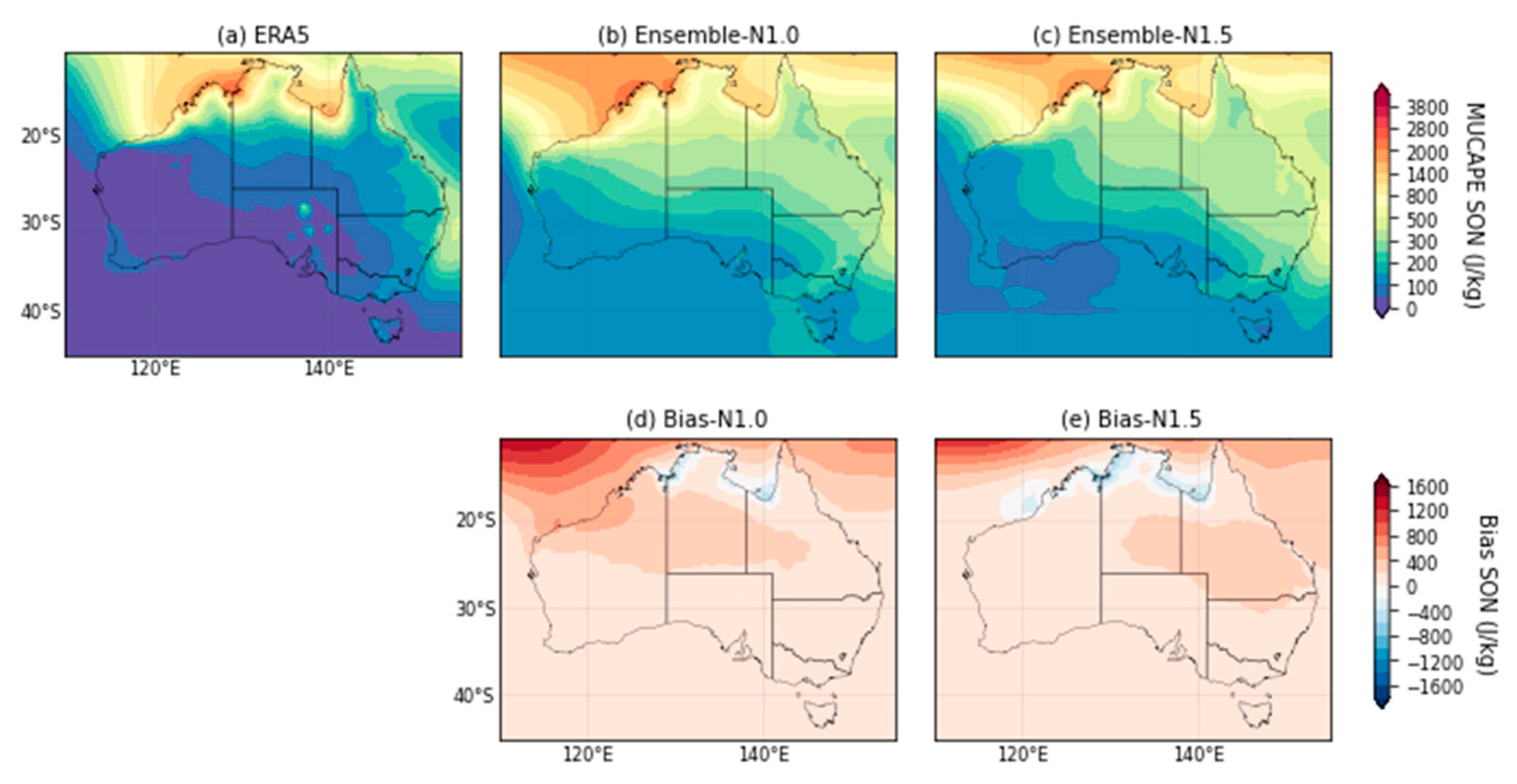
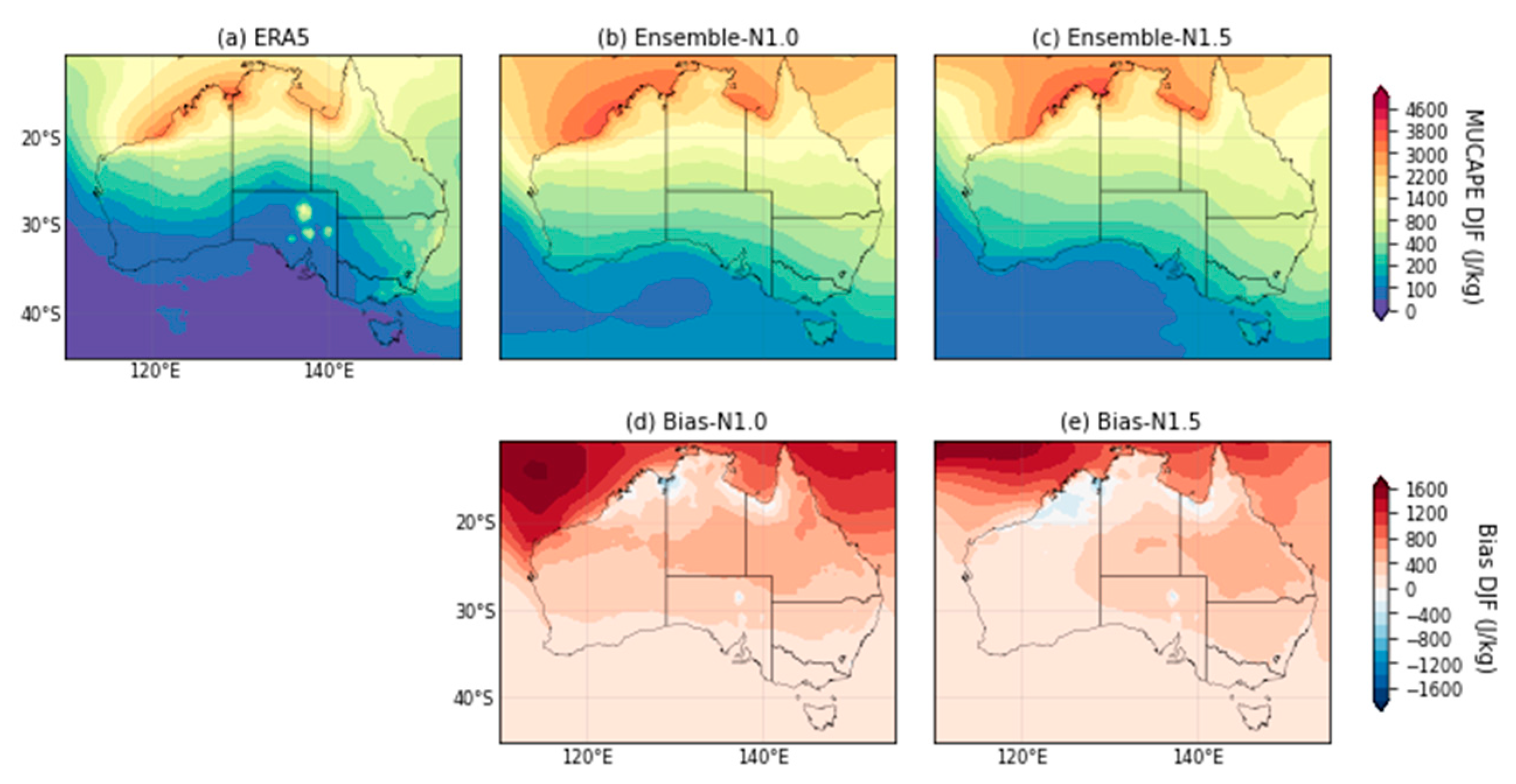
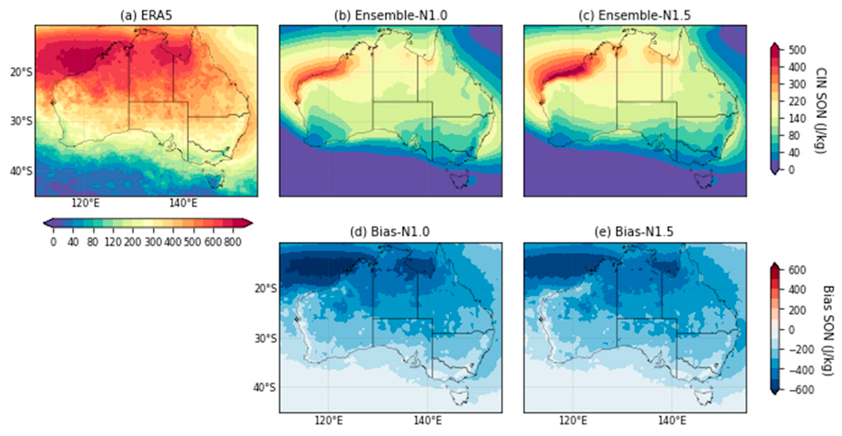
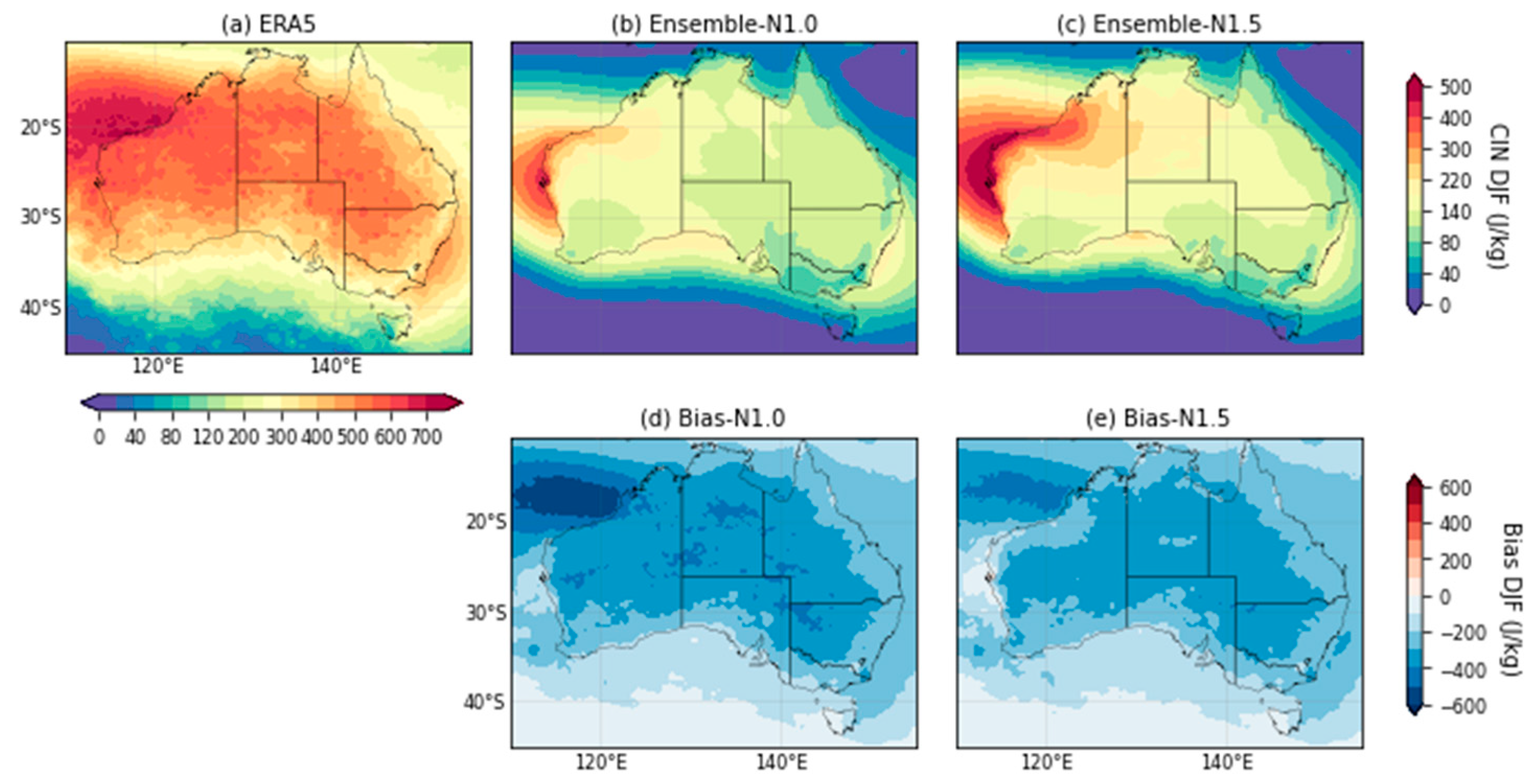
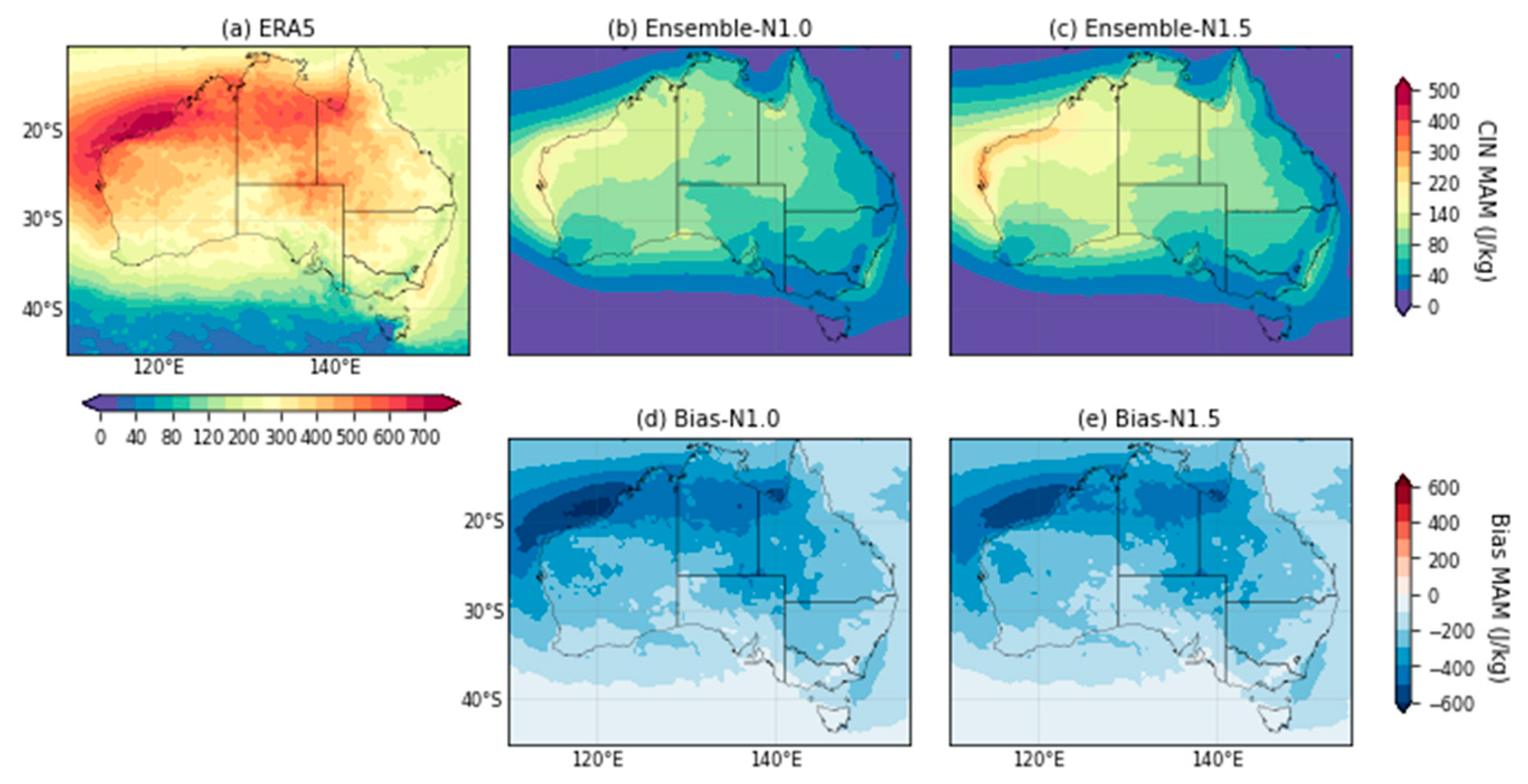
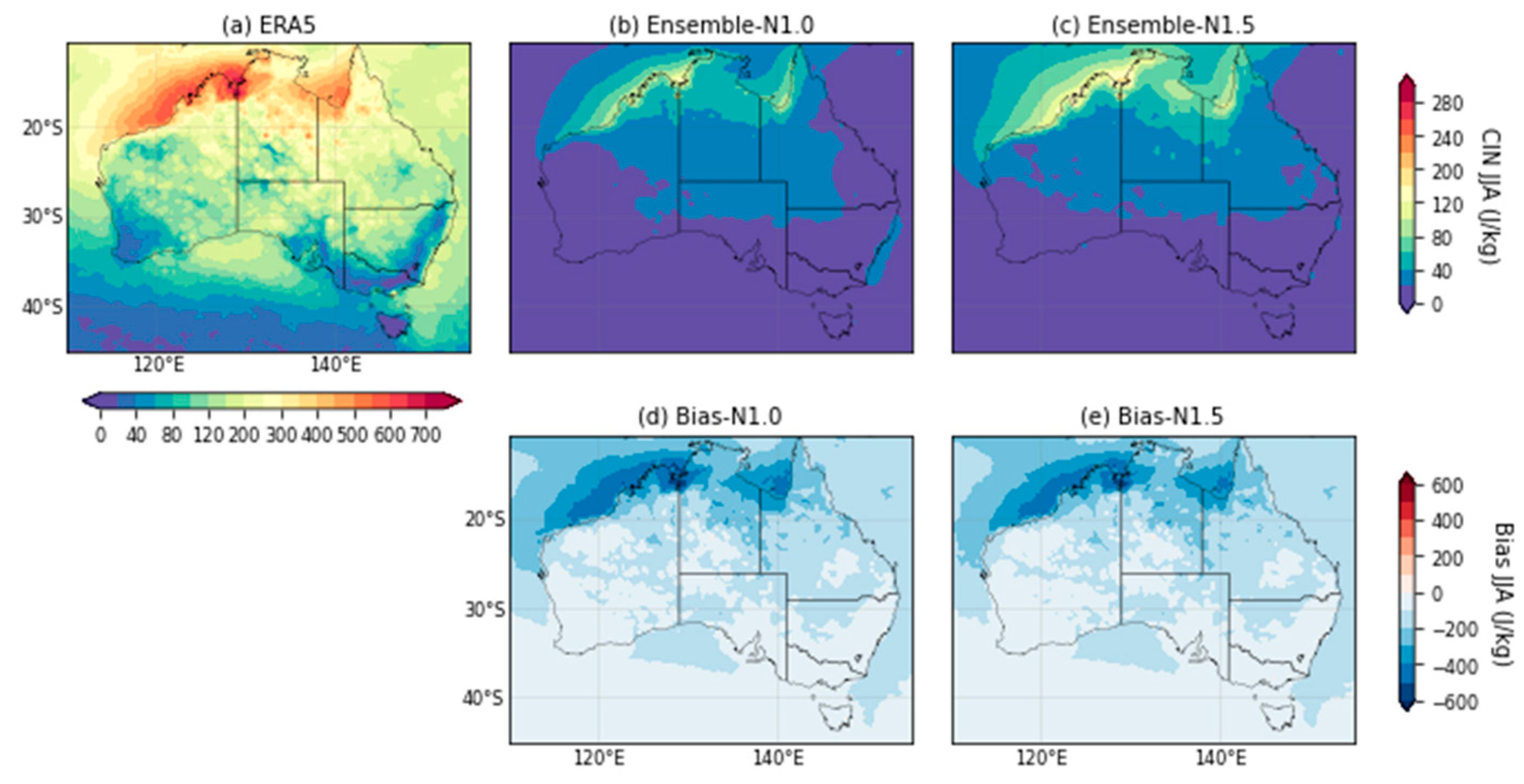
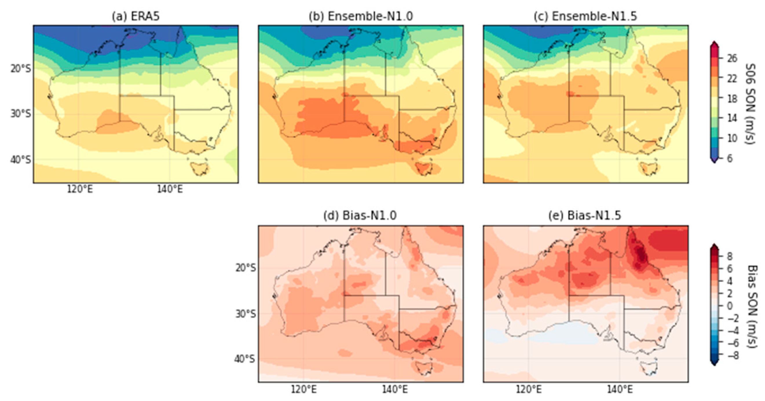
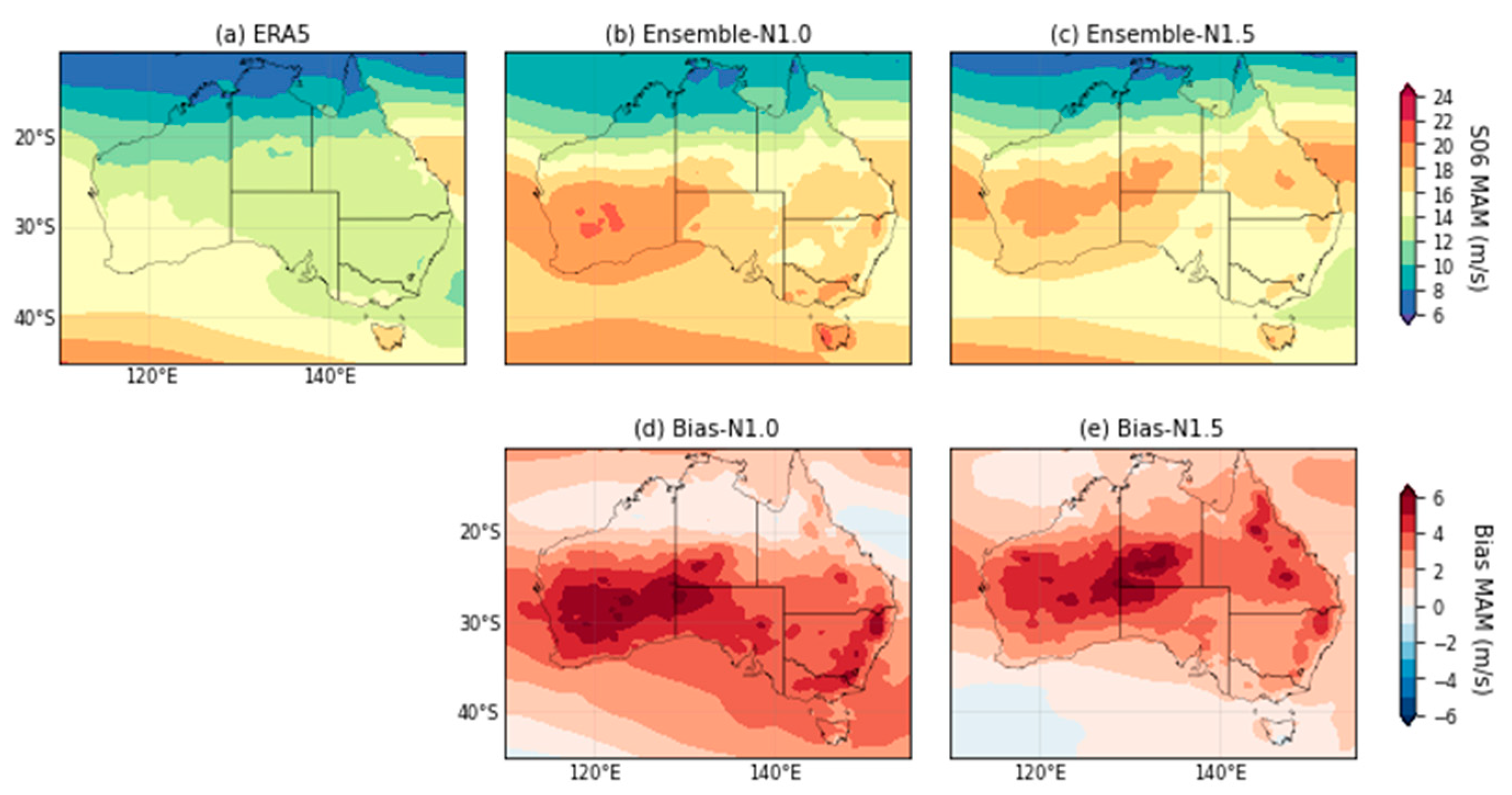
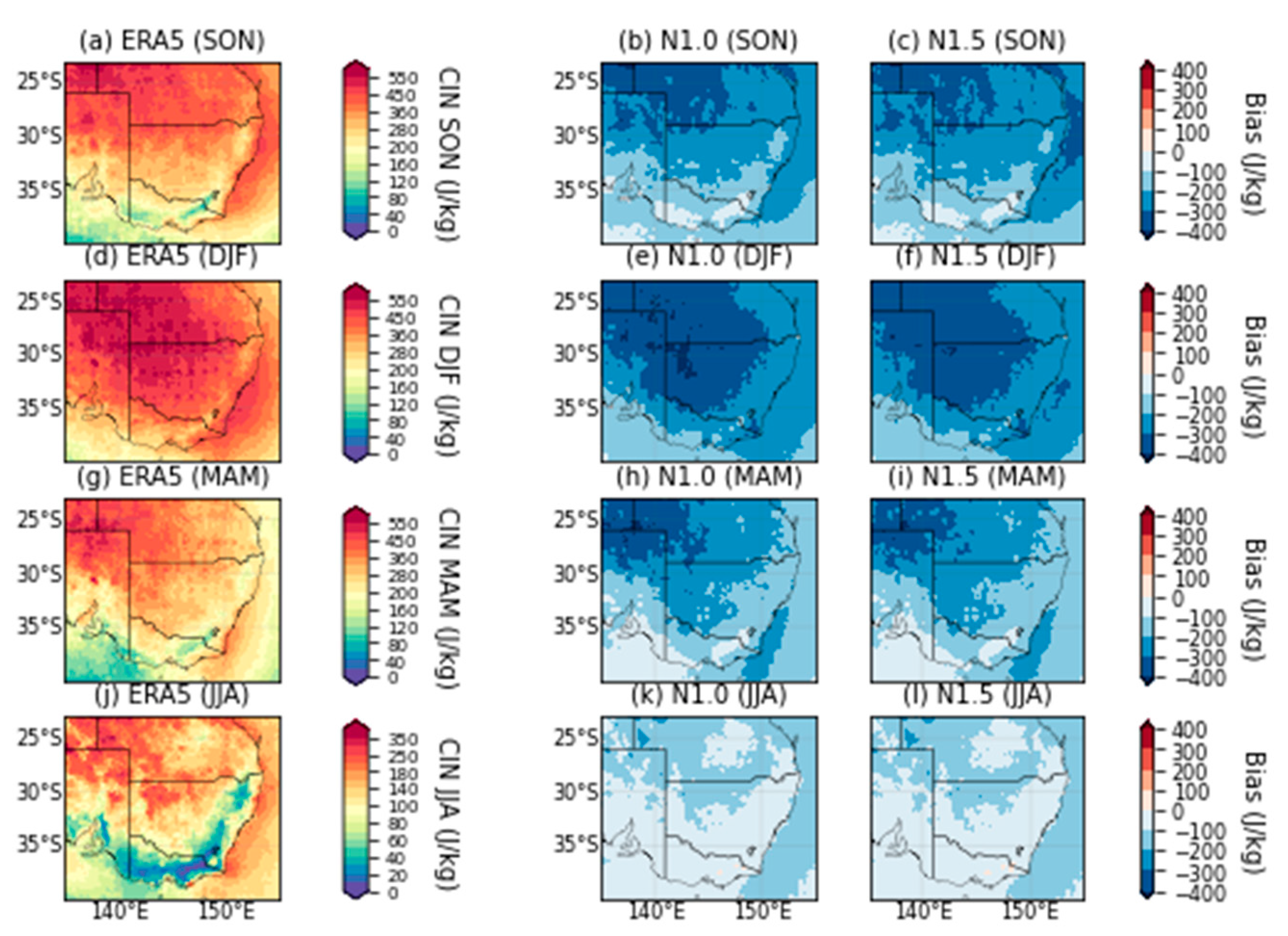
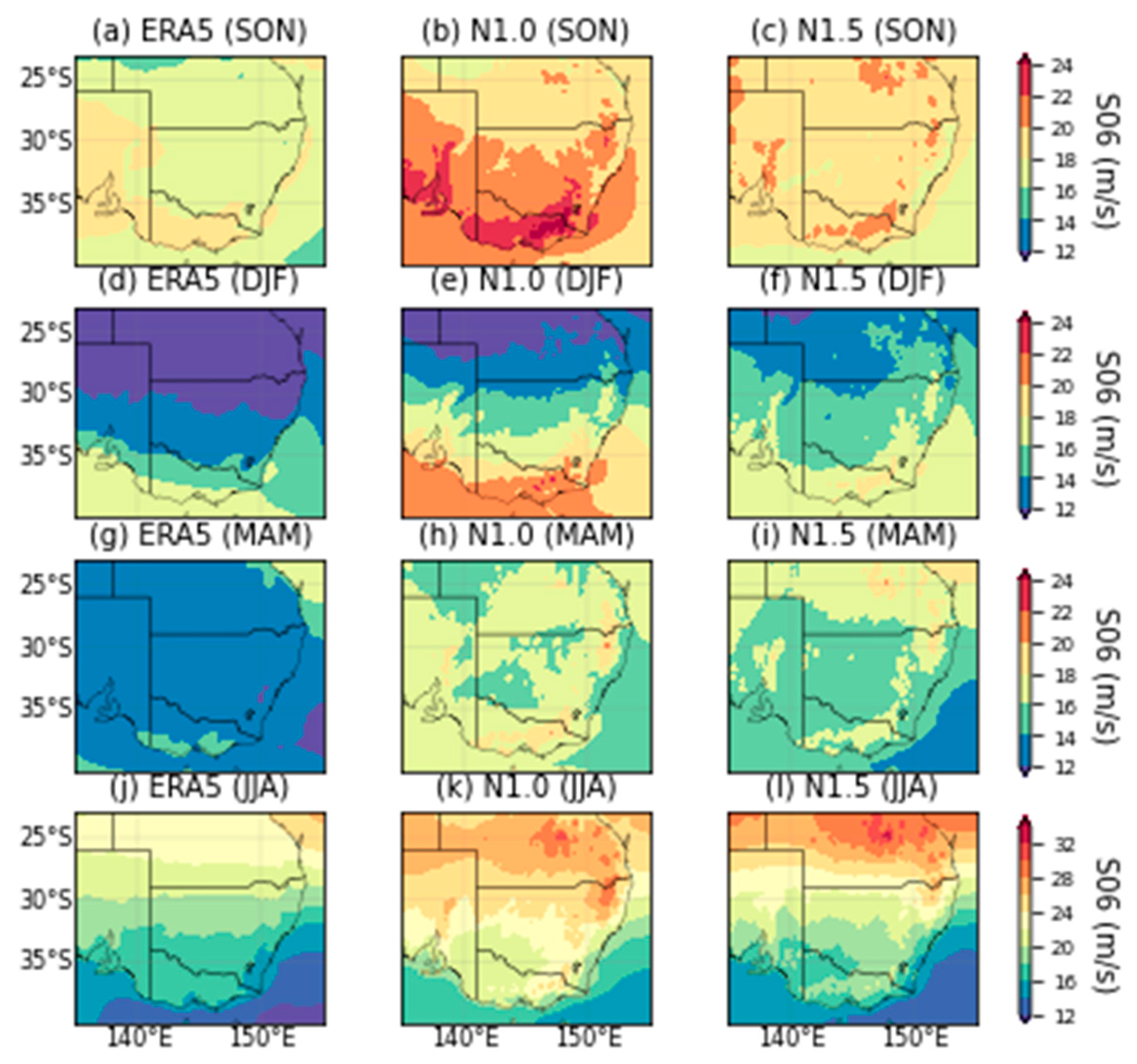
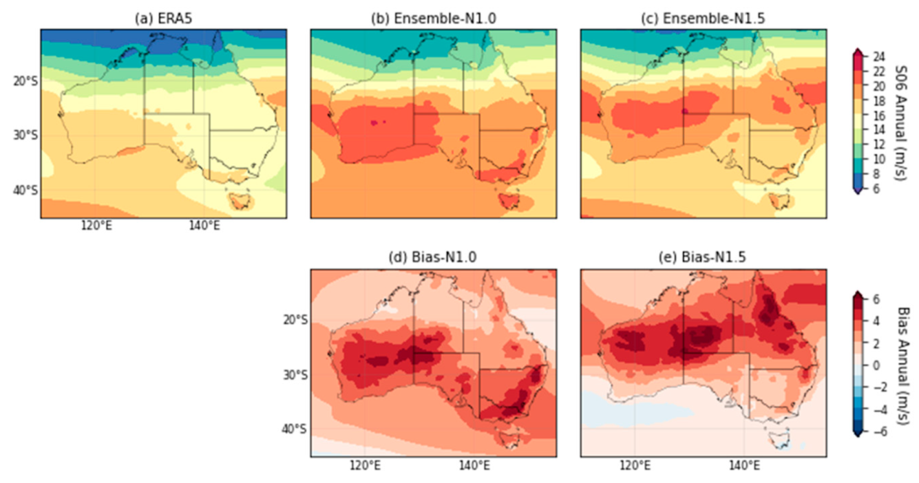
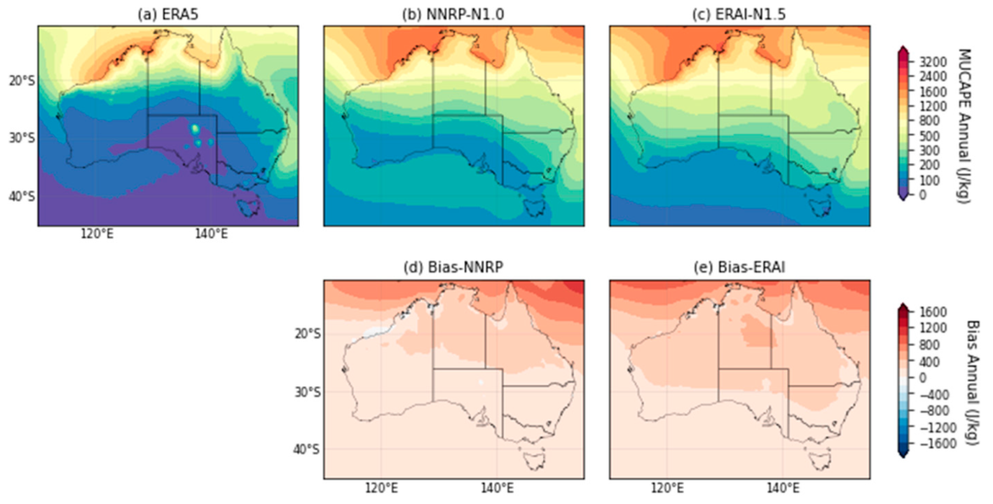
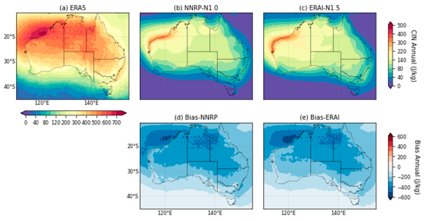
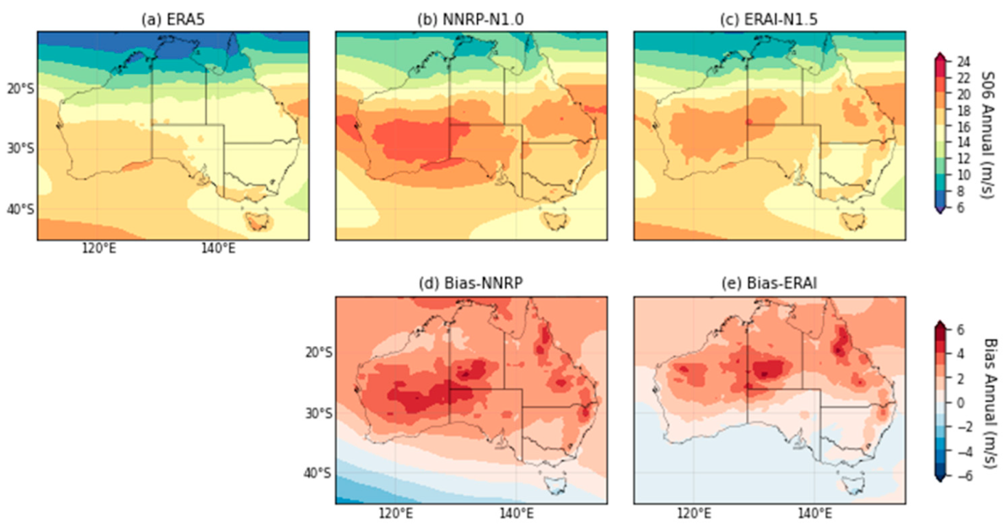
4.1. Climatology and Bias Analysis
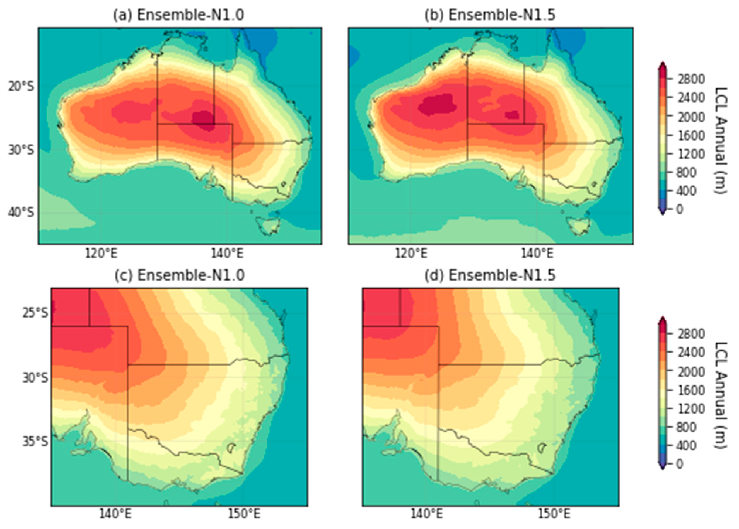
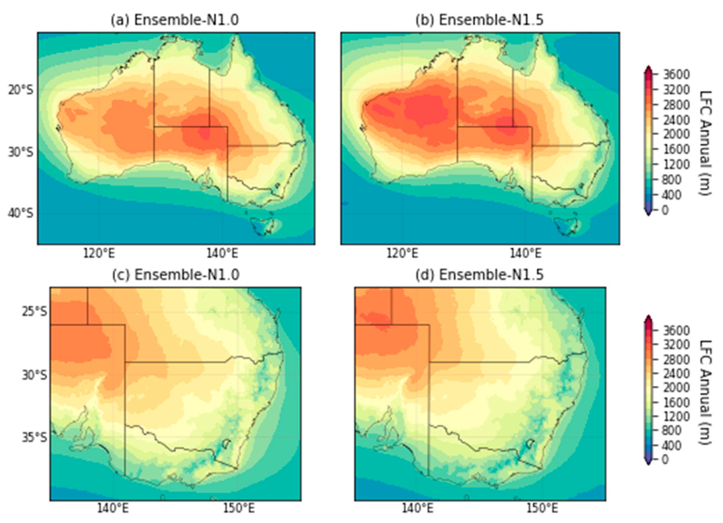
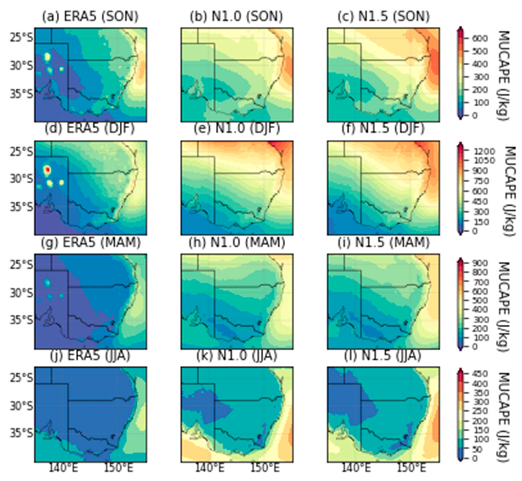
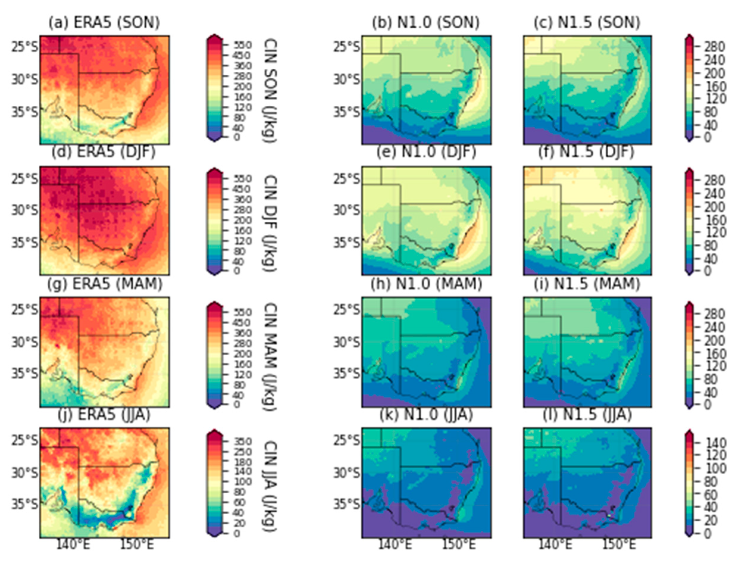
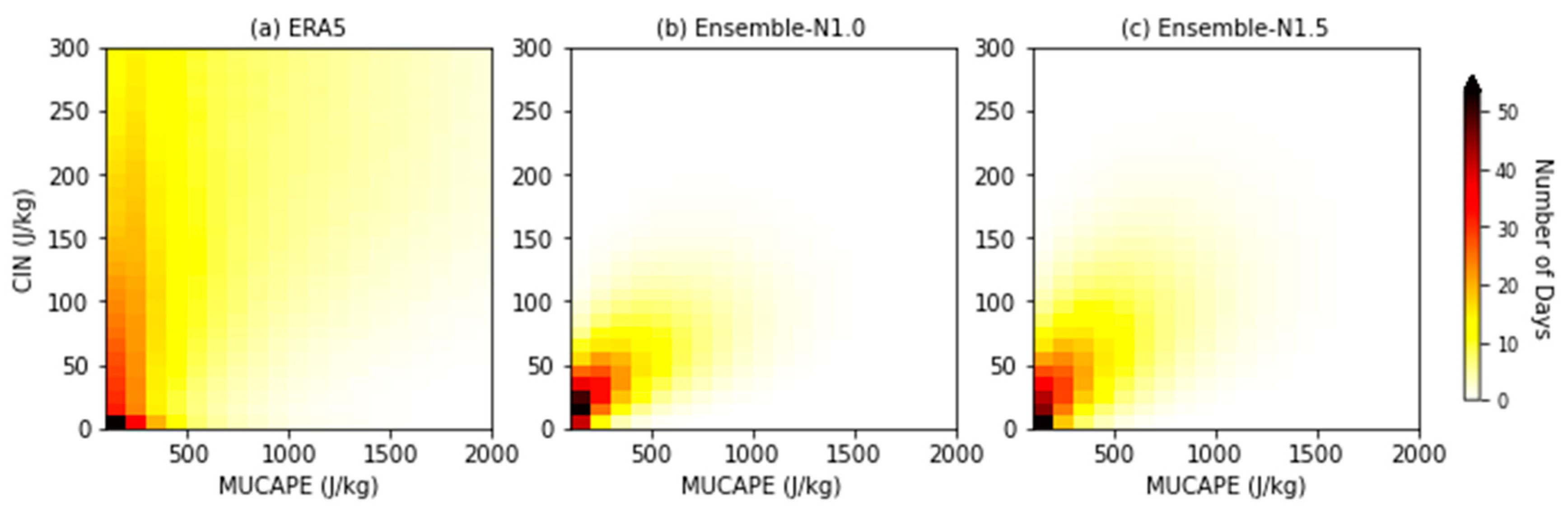
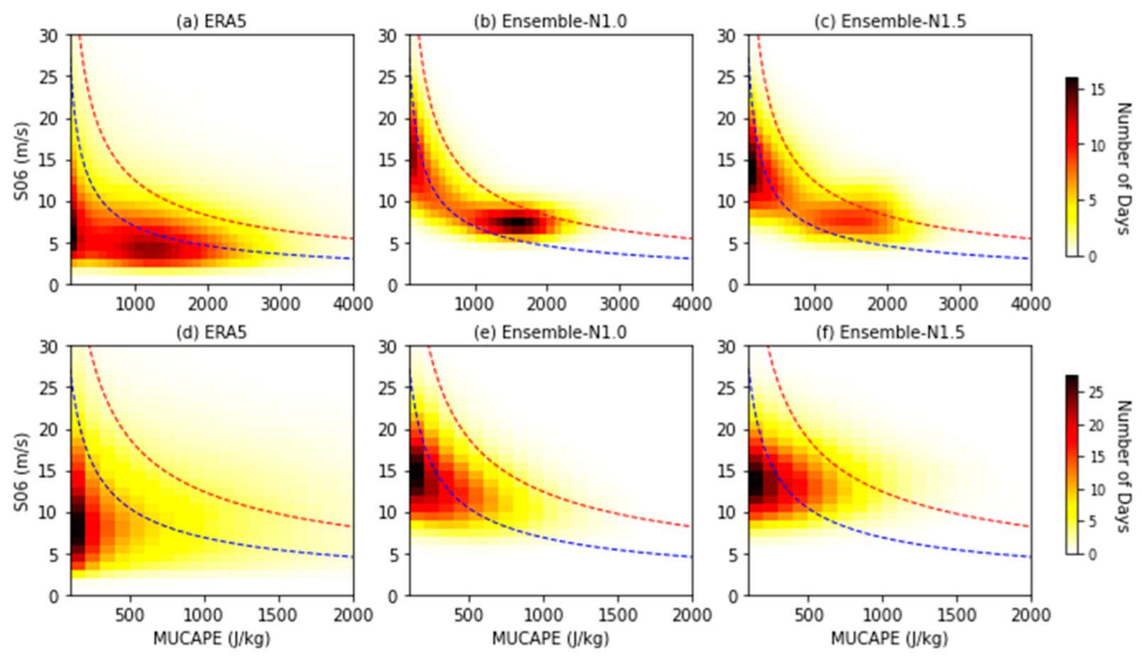
4.2. Convective Environments
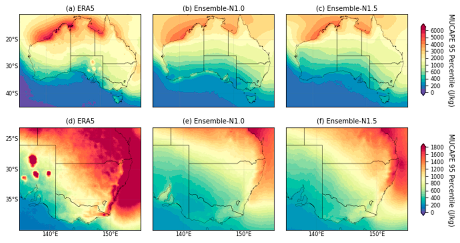
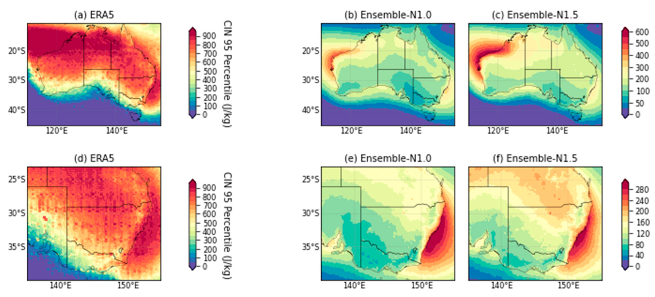
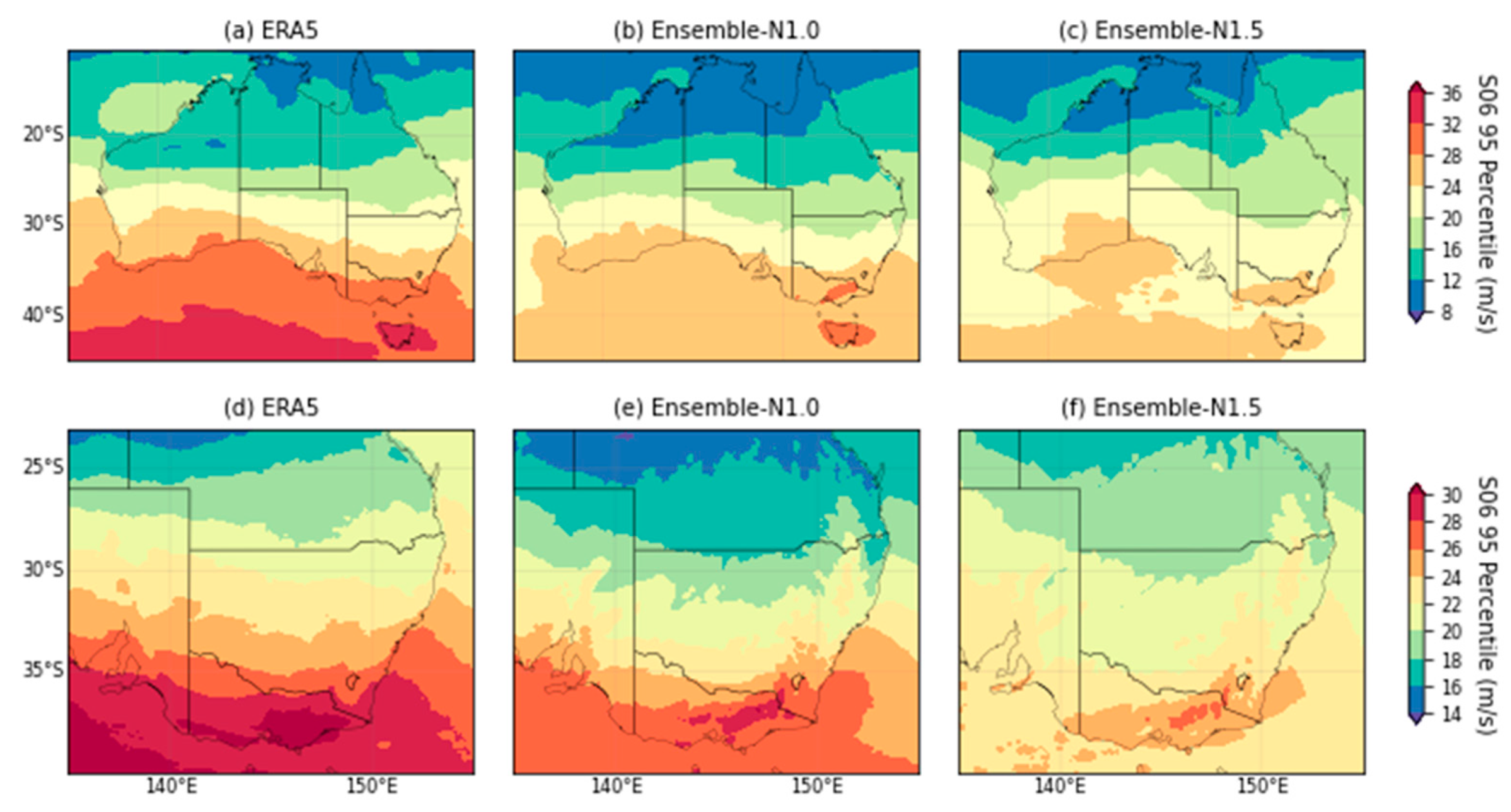
4.3. Extremes
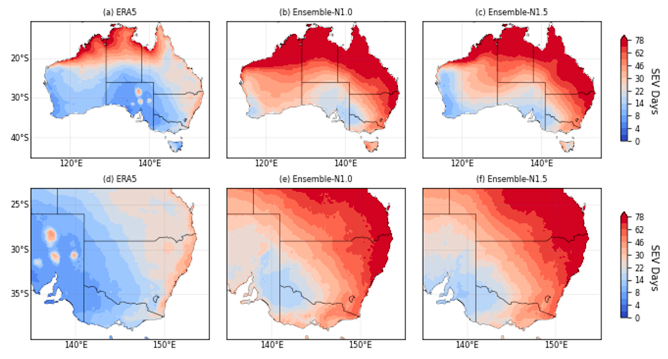
4.4. Storm Days
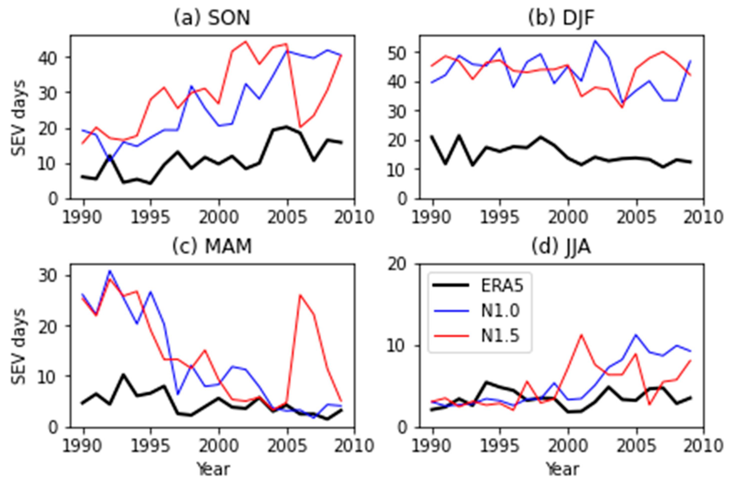
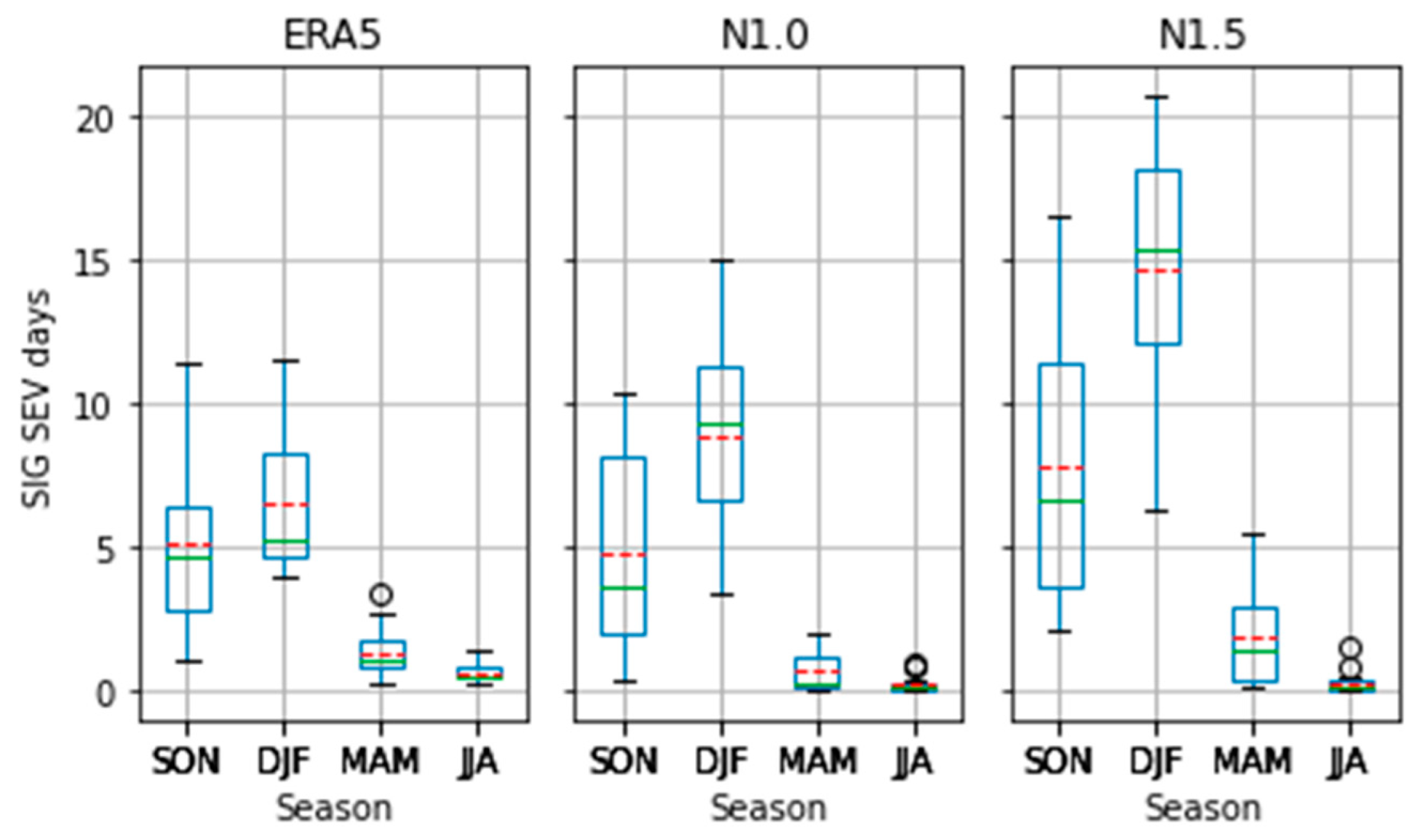
4.5. Seasonal Variation and Interannual Variability
5. Contributions from GCMs and RCMs
6. Summary and Discussion
6.1. Discussion
6.2. Summary
Author Contributions
Funding
Institutional Review Board Statement
Informed Consent Statement
Data Availability Statement
Acknowledgments
Conflicts of Interest
Appendix A

| NARCliM Ensemble Member | Planetary Boundary Layer Physics | Cumulus Physics | Surface Layer Physics | Cloud Microphysics | Shortwave/Longwave Radiation Physics |
|---|---|---|---|---|---|
| R1 | MYJ | KF | Eta similarity | WDM 5 class | Dudhia/RRTM |
| R2 | MYJ | BMJ | Eta similarity | WDM 5 class | Dudhia/RRTM |
| R3 | YSU | KF | MM5 similarity | WDM 5 class | CAM/CAM |
Appendix B
Appendix C


Appendix D


Appendix E
| CIN | MUCAPE | S06 | |||||||
|---|---|---|---|---|---|---|---|---|---|
| Bias | RMSE | PCorr | Bias | RMSE | PCorr | Bias | RMSE | PCorr | |
| N1.0-NNRP | −343.5 | 367.5 | 0.90 | −341.4 | 585.7 | 0.82 | −9.9 | 10.5 | 0.98 |
| N1.0-GCM | −271.7 | 291.5 | 0.88 | 248.8 | 337.6 | 0.91 | 2.7 | 3.0 | 0.99 |
| N1.5-ERAI | −331.7 | 355.1 | 0.85 | −236.6 | 452.8 | 0.95 | −7.7 | 8.2 | 0.97 |
| N1.5-GCM | −256.2 | 272.4 | 0.87 | 216.8 | 297.4 | 0.94 | 3.0 | 3.4 | 0.95 |
| CIN | MUCAPE | S06 | |||||||
|---|---|---|---|---|---|---|---|---|---|
| Bias | RMSE | PCorr | Bias | RMSE | PCorr | Bias | RMSE | PCorr | |
| N1.0-NNRP | −358.3 | 369.3 | 0.94 | −46.7 | 62.5 | 0.75 | −11.0 | 11.0 | 0.38 |
| N1.0-GCM | −293.6 | 302.7 | 0.92 | 180.2 | 201.6 | 0.64 | 3.3 | 3.4 | 0.46 |
| N1.5-ERAI | −347.1 | 358.0 | 0.85 | 1.4 | 41.5 | 0.67 | −10.0 | 10.0 | 0.30 |
| N1.5-GCM | −285.8 | 293.5 | 0.94 | 186.9 | 204.6 | 0.77 | 2.5 | 2.8 | 0.25 |
Appendix F
Appendix G

Appendix H
References
- McAneney, J.; Sandercock, B.; Crompton, R.; Morlock, T.; Musulin, R.; Pielki, R.; Gissing, A. Normalised insurance losses from Australian natural disasters: 1966–2017. Environ. Hazards 2019, 18, 414–433. [Google Scholar] [CrossRef] [Green Version]
- Power, S.; Callaghan, J. Variability in severe coastal flooding, associated storms, and death tolls in southeastern Australia since the mid–nineteenth century. J. Appl. Meteorol. Climatol. 2016, 55, 1139–1149. [Google Scholar] [CrossRef]
- Walsh, K.; White, C.J.; McInnes, K.; Holmes, J.; Schuster, S.; Richter, H.; Evans, J.P.; Di Luca, A.; Warren, R.A. Natural hazards in Australia: Storms and hail. Clim. Chang. 2016, 139, 55–67. [Google Scholar] [CrossRef] [Green Version]
- Groenemeijer, P.; Púčik, T.; Holzer, A.M.; Antonescu, B.; Riemann-Campe, K.; Schultz, D.M.; Kühne, T.; Feuerstein, B.; Brooks, H.E.; Doswell, C.A., III; et al. Severe convective storms in Europe. Bull. Am. Meteorol. Soc. 2017, 98, 2641–2651. [Google Scholar] [CrossRef]
- Dowdy, A.; Soderholm, J.; Brook, J.; Brown, A.; McGowan, H. Quantifying hail and lightning risk factors using long-term observations around Australia. J. Geophys. Res. Atmos. 2020, 125, 2020JD033101. [Google Scholar] [CrossRef]
- Taszarek, M.; Allen, J.T.; Groenemeijer, P.; Edward, R.; Brooks, H.E.; Chmielewski, V.; Enno, S.-E. Severe convective storms across Europe and the United States. Part I: Climatology of lightning, large hail, severe wind, and tornadoes. J. Clim. 2020, 33, 10239–10260. [Google Scholar] [CrossRef]
- Taszarek, M.; Allen, J.T.; Marchio, M.; Brooks, H.E. Global climatology and trends in convective environments from ERA5 and rawinsonde data. Npj Clim. Atmos. Sci. 2021, 4, 35. [Google Scholar] [CrossRef]
- Dowdy, A. Seasonal forecasting of lightning and thunderstorm activity in tropical and temperate regions of the world. Sci. Rep. 2016, 6, 20874. [Google Scholar] [CrossRef] [Green Version]
- Allen, J.; Allen, E.R. A review of severe thunderstorms in Australia. Atmos. Res. 2016, 178–179, 347–366. [Google Scholar] [CrossRef] [Green Version]
- Doswell, C.A. The distinction between large-scale and mesoscale contribution to severe convection: A case study example. Weather Forecast. 1987, 2, 3–16. [Google Scholar] [CrossRef]
- Doswell, C.A.; Brooks, H.E.; Maddox, R. Flash flood forecasting: An ingredients-based methodology. Weather Forecast. 1996, 11, 560–581. [Google Scholar] [CrossRef]
- Bednarczyk, C.N.; Sousounis, P.J. Hail climatology of Australia based on lightning and reanalysis. In Proceedings of the 27th Conference on Severe Local Storms, Santa Fe, NM, USA, 24–28 October 2022; American Meteorological Society: Madison, MI, USA, 2012; Volume 142. [Google Scholar]
- Dowdy, A.; Kuleshov, Y. Climatology of lightning activity in Australia: Spatial and seasonal variability. Aust. Meteorol. Oceanogr. Soc. 2014, 64, 103–108. [Google Scholar] [CrossRef]
- Rasuly, A.A.; Cheung, K.; McBurney, B. Hail events across the Greater Metropolitan severe thunderstorm warning area. Nat. Haz. Earth Syst. Sci. 2015, 15, 973–984. [Google Scholar] [CrossRef] [Green Version]
- Raupach, T.H.; Martius, O.; Allen, J.T.; Kunz, M.; Lasher-Trapp, S.; Mohr, S.; Rasmussen, K.L.; Trapp, R.J.; Zhang, Q. The effects of climate change on hailstorms. Nat. Rev. 2021, 2, 213–226. [Google Scholar] [CrossRef]
- Rasmussen, K.L.; Prein, A.F.; Rasmussen, R.M.; Ikeda, K.; Liu, C. Changes in the convective population and thermodynamic environments in convection-permitting regional climate simulations over the United States. Clim. Dyn. 2020, 55, 383–408. [Google Scholar] [CrossRef]
- Buckley, B.W.; Leslie, L.M.; Wang, Y. The Sydney Hailstorm of April 14, 1999: Synoptic description and numerical simulation. Meteorol. Atmos. Phys. 2001, 76, 167–182. [Google Scholar] [CrossRef]
- Leslie, L.M.; Leplastrier, M.; Buckley, B.W. Estimating future trends in severe hailstorms over the Sydney basin: A climate modelling study. Atmos. Res. 2008, 87, 37–51. [Google Scholar] [CrossRef]
- Hartigan, J.; MacNamara, S.; Leslie, L.M.; Speer, M.S. High-resolution simulations of a tornadic storm affecting Sydney. ANZIAM J. 2021, 62, C1–C15. [Google Scholar] [CrossRef]
- Allen, J.; Karoly, D.; Walsh, K. Future Australian severe thunderstorm environments. Part I: A novel evaluation and climatology of convective parameters from two climate models for the late twentieth century. J. Clim. 2014, 27, 3827–3847. [Google Scholar] [CrossRef]
- Evans, J.P.; Ji, F.; Lee, C.; Smith, P.; Argüeso, D.; Fita, L. Design of a regional climate modelling projection ensemble experiment—NARCliM. Geosci. Model Dev. 2014, 7, 621–629. [Google Scholar] [CrossRef] [Green Version]
- Solomon, S.; Qin, D.; Manning, M.; Averyt, K.; Marquis, M. Climate Change 2007: The Physical Science Basis. Contribution of Working Group I to the Fourth Assessment Report of the Intergovernmental Panel on Climate Change; Cambridge University Press: Cambridge, UK; New York, NY, USA, 2007. [Google Scholar]
- Kalnay, E.; Kanamitsu, M.; Kistler, R.; Collins, W.; Deaven, D.; Gandin, L.; Iredell, M.; Saha, S.; White, G.; Woollen, J.; et al. The NCEP/NCAR 40-year reanalysis project. Bull. Am. Meteorol. Soc. 1996, 77, 437–471. [Google Scholar] [CrossRef]
- Nishant, N.; Evans, J.P.; Virgilio, G.; Downes, S.M.; Ji, F.; Cheung, K.K.W.; Tam, E.; Miller, J.; Beyer, K.; Riley, M.L. Introducing NARCliM1.5: Evaluating the Performance of Regional Climate Projections for Southeast Australia for 1950–2100. Earth’s Future 2021, 9, 2020EF001833. [Google Scholar] [CrossRef]
- Dee, D.P.; Uppala, S.M.; Simmons, A.J.; Berrisford, P.; Poli, P.; Kobayashi, S.; Andrae, U.; Balmaseda, M.A.; Balsamo, G.; Bauer, P.; et al. The ERA-Interim reanalysis: Configuration and performance of the data assimilation system. Quart. J. R. Meteorol. Soc. 2011, 137, 553–597. [Google Scholar] [CrossRef]
- Ji, F.; Evans, J.P.; Teng, J.; Scorgie, Y.; Argüeso, D.; Di Luca, A. Evaluation of long-term precipitation and temperature Weather Research and Forecasting simulations for southeast Australia. Clim. Res. 2016, 67, 99–115. [Google Scholar] [CrossRef] [Green Version]
- Fita, L.; Evans, J.P.; Argüeso, D.; Liu, Y. Evaluation of the regional climate response in Australia to large-scale climate models in the historical NARCliM simulations. Clim. Dyn. 2016, 49, 2815–2829. [Google Scholar] [CrossRef]
- Ji, F.; Nishant, N.; Evans, J.P.; Di Virgilio, G.; Cheung, K.K.W.; Tam, E.; Beyer, K.; Riley, M.L. Introducing NARCliM1.5: Evaluation and projection of climate extremes for Southeast Australia. Weather Clim. Extrem. 2022, 38, 100526. [Google Scholar] [CrossRef]
- Romps, D. Exact expression for the lifting condensation level. J. Atmos. Sci. 2017, 74, 3891–3900. [Google Scholar] [CrossRef]
- Moncrieff, M.W.; Miller, M.J. The dynamics and simulation of tropical cumulonimbus and squall lines. Quart. J. R. Meteorol. Soc. 1976, 102, 373–394. [Google Scholar] [CrossRef]
- Mapes, B. Convective inhibition, subgrid-scale triggering energy, and stratiform instability in a toy tropical wave model. J. Atmos. Sci. 2000, 57, 1515–1535. [Google Scholar] [CrossRef]
- Bunkers, M.J.; Klimowski, B.A.; Zeitler, J.W. The importance of parcel choice and the measure of vertical wind shear in evaluating the convective environment. In Proceedings of the Extended Abstracts, 21st Conference on Severe Local Storms, Savannah, GA, USA, 12–16 August 2002; Severe Local Storms, San Antonio, American Meteorological Society: San Antonio, TX, USA, 2002; p. 8.2. [Google Scholar]
- Taszarek, M.; Pilguj, N.; Allen, J.T.; Gensini, V.; Brooks, H.E.; Szuster, P. Comparison of convective parameters derived from ERA5 and MERRA-2 with rawinsonde data over Europe and North America. J. Clim. 2021, 34, 3211–3237. [Google Scholar]
- Allen, J.; Karoly, D.; Mills, G.A. Severe thunderstorm climatology for Australia and associated thunderstorm environments. Aust. Meteorol. Oceanogr. J. 2011, 61, 143–158. [Google Scholar] [CrossRef]
- Allen, J.; Karoly, D. A climatology of Australian severe thunderstorm environments 1979-2011: Inter-annual variability and ENSO influence. Int. J. Climatol. 2014, 34, 81–97. [Google Scholar] [CrossRef]
- Prein, A.F.; Holland, G.J. Global estimates of damaging hail hazard. Weather Clim. Extrem. 2018, 22, 10–23. [Google Scholar] [CrossRef]
- Colman, B.R. Thunderstorms above frontal surfaces in environments without positive CAPE. Part I: A climatology. Mon. Weather Rev. 1990, 118, 1103–1121. [Google Scholar] [CrossRef]
- Colman, B.R. Thunderstorms above frontal surfaces in environments without positive CAPE. Part II: Organization and instability mechanisms. Mon. Weather Rev. 1990, 118, 1123–1144. [Google Scholar] [CrossRef]
- Thompson, R.; Mead, C.M.; Edwards, R. Effective storm-relative helicity and bulk shear in supercell thunderstorm environments. Weather Forecast. 2007, 22, 102–115. [Google Scholar] [CrossRef]
- Weisman, M.L.; Klemp, J.B. The dependence of numerically simulated convective storms on vertical wind shear and buoyancy. Mon. Weather Rev. 1982, 110, 504–520. [Google Scholar] [CrossRef]
- Brooks, H.E.; Lee, J.W.; Craven, J.P. The spatial distribution of severe thunderstorm and tornado environments from global reanalysis data. Atmos. Res. 2003, 67–68, 73–94. [Google Scholar] [CrossRef]
- Van Zomeren, J.; van Delden, A. Vertically integrated moisture flux convergence as a predictor of thunderstorms. Atmos. Res. 2007, 83, 435–445. [Google Scholar] [CrossRef]
- Koch, E.; Koh, J.; Davison, A.C.; Lepore, C.; Tippett, M.K. Trends in the extremes of environments associated with severe U.S. thunderstorms. J. Clim. 2021, 34, 1259–1272. [Google Scholar] [CrossRef]
- Allen, J.; Karoly, D.; Walsh, K. Future Australian severe thunderstorm environments. Part II: The influence of a strongly warming climate on convective environments. J. Clim. 2014, 27, 3848–3868. [Google Scholar] [CrossRef]
- Hersbach, H.; Bell, B.; Berrisford, P.; Hirahara, S.; Horányi, A.; Muñoz-Sabater, J.; Nicolas, J.; Peubey, C.; Radu, R.; Schepers, D.; et al. The ERA5 global reanalysis. Quart. J. R. Meteorol. Soc. 2020, 146, 1999–2049. [Google Scholar] [CrossRef]
- Vicente-Serrano, S.M.; García-Herrera, R.; Peña-Angulo, D.; Tomas-Burguera, M.; Domínguez-Castro, F.; Noguera, I.; Calvo, N.; Murphy, C.; Nieto, R.; Gimeno, L.; et al. Do CMIP models capture long-term observed annual precipitation trends? Clim. Dyn. 2022, 58, 2825–2842. [Google Scholar] [CrossRef]
- Chen, W.; Jiang, Z.; Li, L. Probabilistic projections of climate change over China under the SRES A1B scenario using 28 AOGCMs. J. Clim. 2011, 24, 4741–4756. [Google Scholar] [CrossRef] [Green Version]
- Chen, J.; Dai, A.; Zhang, Y.; Rasmussen, K.L. Changes in convective available potential energy and convective inhibition under global warming. J. Clim. 2020, 33, 2025–2050. [Google Scholar] [CrossRef]
- DPE. Projecting Storm Environment under Climate Change—Evaluation Report; Climate Research, Climate and Atmospheric Science, NSW Department of Planning and Environment, Environment, Energy and Science: Sydney, NSW, Australia, 2023.
- Taszarek, M.; Allen, J.T.; Pucik, T.; Hoogewind, K.A.; Brooks, H.E. Severe convective storms across Europe and the United States. Part II: ERA5 environments associated with lightning, large hail, severe wind, and tornadoes. J. Clim. 2020, 33, 10263–10286. [Google Scholar] [CrossRef]
- Wang, Z.; Franke, J.A.; Luo, Z.; Moyer, E.J. Reanalysis and a high-resolution model fail to capture the “high-tail” of CAPE distribution. J. Clim. 2021, 34, 8699–8715. [Google Scholar] [CrossRef]
- Trapp, R.J.; Diffenbaugh, N.S.; Brooks, H.E.; Baldwin, M.E.; Robinson, E.D.; Pal, J.S. Changes in severe thunderstorm environment frequency during the 21st century caused by anthropogenically enhanced global radiative forcing. Proc. Nat. Acad. Sci. USA 2007, 104, 19719–19723. [Google Scholar] [CrossRef] [Green Version]
- Ji, F.; Nishant, N.; Evans, J.P.; Di Luca, A.; Di Virgilio, G.; Cheung, K.K.W.; Tam, E.; Beyer, K.; Riley, M.L. Rapid warming in the Australian Alps from observation and NARCliM simulations. Atmosphere 2022, 13, 1686. [Google Scholar] [CrossRef]
- Pilguj, N.; Taszarek, M.; Allen, J.T.; Hoogewind, K.A. Are trends in convective parameters over the United States and Europe consistent between reanalyses and observations? J. Clim. 2022, 35, 3605–3626. [Google Scholar] [CrossRef]
- Varga, A.J.; Breuer, H. Evaluation of convective parameters derived from pressure level and native ERA5 data and different resolution WRF climate simulations over Central Europe. Clim. Dyn. 2022, 58, 1569–1585. [Google Scholar] [CrossRef]
- Herold, N.; Downes, S.M.; Gross, M.H.; Ji, F.; Nishant, N.; Macadam, I.; Ridder, N.N.; Beyer, K. Projected changes in the frequency of climate extremes over southeast Australia. Environ. Res. Lett. 2021, 3, 011001. [Google Scholar] [CrossRef]


| SON | DJF | MAM | JJA | |
|---|---|---|---|---|
| N1.0 (d01) | 0.07 | 0.14 | 0.59 | 0.50 |
| N1.5 (d01) | 0.16 | 0.01 | 0.02 | 0.39 |
| N1.0 (d02) | 0.02 | 0.25 | 1.20 | 1.26 |
| N1.5 (d02) | 0.01 | 0.01 | 1.99 | 0.70 |
Disclaimer/Publisher’s Note: The statements, opinions and data contained in all publications are solely those of the individual author(s) and contributor(s) and not of MDPI and/or the editor(s). MDPI and/or the editor(s) disclaim responsibility for any injury to people or property resulting from any ideas, methods, instructions or products referred to in the content. |
© 2023 by the authors. Licensee MDPI, Basel, Switzerland. This article is an open access article distributed under the terms and conditions of the Creative Commons Attribution (CC BY) license (https://creativecommons.org/licenses/by/4.0/).
Share and Cite
Cheung, K.K.W.; Ji, F.; Nishant, N.; Herold, N.; Cook, K. Evaluation of Convective Environments in the NARCliM Regional Climate Modeling System for Australia. Atmosphere 2023, 14, 690. https://doi.org/10.3390/atmos14040690
Cheung KKW, Ji F, Nishant N, Herold N, Cook K. Evaluation of Convective Environments in the NARCliM Regional Climate Modeling System for Australia. Atmosphere. 2023; 14(4):690. https://doi.org/10.3390/atmos14040690
Chicago/Turabian StyleCheung, Kevin K. W., Fei Ji, Nidhi Nishant, Nicholas Herold, and Kellie Cook. 2023. "Evaluation of Convective Environments in the NARCliM Regional Climate Modeling System for Australia" Atmosphere 14, no. 4: 690. https://doi.org/10.3390/atmos14040690