Article

Detection of Air Pollution in Urban Areas Using Monitoring Images

1
Department of Artificial Intelligence, Shenzhen University, Shenzhen 518060, China
2
Department of Mathematics and Information Technology, The Education University of Hong Kong, Hong Kong, China
3
Department of Electrical and Computer Engineering, University of Massachusetts Lowell, Lowell, MA 01854, USA
*
Author to whom correspondence should be addressed.
Atmosphere 2023, 14(5), 772; https://doi.org/10.3390/atmos14050772
Submission received: 5 April 2023 / Revised: 12 April 2023 / Accepted: 21 April 2023 / Published: 23 April 2023
(This article belongs to the Section Air Quality)

Abstract

:
Air quality monitoring in polluted environments is of great significance to human health. Traditional methods use various pieces of meteorological equipment, which have limited applications in complex terrains and high costs. In this paper, a novel idea is put forward to solve the problem of air pollution monitoring in urban areas. We investigate whether air quality can be assessed visually by examining the haziness of photos from a far distance. Specifically, the correlation between the air quality indexes, such as the AQI, PM2.5, and PM10, of real outdoor scenarios and the haziness level evaluation scores of the monitoring images is calculated. The results show that the objective indicators can indeed reflect the level of air pollution, and the degree of correlation is invariant to the image size. To apply this new observation to a practical system, a novel method called fastDBCP (fast dark and bright channel prior) is developed. Based on a down-sampling strategy, a ratio is calculated between the dark and bright channel prior information in scaled images and adopted as the visual index of air pollution. Our experimental results show that the proposed metric not only demonstrates advantages in terms of its correlation degree and computational speed, but also shows a high level of classification accuracy compared to that of competing metrics.

1. Introduction

Outdoor haze is a well-known weather phenomenon. Traditionally, meteorologists monitor air quality with a variety of instruments and equipment. Popular indicators such as the AQI, PM2.5, and PM10 have been widely used to determine the quality of air. The advantage of these means is their high accuracy, while the disadvantage is that the distribution of the instruments is limited by the terrain, and it is difficult and costly in some areas, such as in mountains and deserts. In addition, the calculation of indicators requires data from various pieces of monitoring equipment. Hence, it is difficult to make real-time judgments. Although it may not be easy to solve the above problems by traditional meteorologic means, we can look at the problem from another angle. Researchers have been exploring various solutions in terms of vision. For instance, Sallis et al. suggested using vehicular sensors to detect air pollution and fog [1], Wong et al. used surveillance cameras to determine the temporal patterns of the PM10 concentration in the air [2], and Mukundan et al. proposed an air pollution detection method using snapshot hyperspectral imaging [3].
In this paper, we present a novel method to detect air pollution from monitoring images, which was inspired by the above vision-oriented methods. The differences are that our method does not need extra signals, such as sensors or hyperspectral data, and it covers a wider range of air quality categories. The rationale of the idea is twofold. First, thanks to the widespread development of imaging technology, monitoring videos/photos can be easily obtained through lenses, especially in urban areas. Second, in the field of image quality assessment, there are many effective objective evaluation indicators [4,5,6,7,8,9,10,11]. Of course, image quality cannot be simply treated as air quality. However, previous research studies have shown that certain image quality evaluation indicators can indeed characterize the haze level effectively [12,13,14,15,16], which is relevant to the air quality in hazy weather. Some implicit relationships between the subjective scores in hazy images and the corresponding environmental indicators were revealed in our previous work [17].
Based on the existing research findings, it is natural to ask: for hazy weather, does the image quality of a photo have a high correlation with the air quality at that time? Can such an indicator be used to characterize the level of air pollution? Our answer is yes, because physically the light source irradiates the object that is photographed, and the light reflected by the object is refracted or scattered by air particles to make an integral projection on the image perceptron. Assuming that the object and the light source are unchanged, the painting is equivalent to adding a filter to the reflected light of the object, and various components in the air will affect the performance of the filter, resulting in different images. Meanwhile, the composition of the air is related to the quality of the air. Hence, the quality of the air can be inferred by analyzing the differences in the images.
To confirm the aforementioned analysis, we performed experiments to explore the relationship between objective evaluation indicators and air quality indexes on our newly upgraded database called RHID_AQI [16]. The dataset includes real outdoor pictures taken in eight city environments. Compared to the former version, the upgraded dataset supplemented the air pollution level for each picture on the day it was taken. The experimental results are encouraging. A strong correlation between image quality and air pollution level is discovered. Hence, a fast evaluation system that reflects air quality through monitoring photos in urban areas is proposed in this paper. The main measure is to introduce a down-sampling strategy and utilize the dark channel and bright channel information in a hazy image. The new system is simple but effective, and the speed of the air quality evaluation is satisfactory.
The rest of the paper is organized as follows. The proposed method is described in detail in Section 2. In Section 3, we compare and analyze the performance of our metric compared to state-of-the-art indicators. In Section 4, possible applications in the field of air pollution monitoring and other types of real-time monitoring systems are investigated, and the conclusions are drawn in Section 5.

2. Dataset and Method

2.1. RHID_AQI Dataset

The RHID_AQI dataset was built by our team to provide a public benchmark to blindly evaluate the image quality of hazy images [16,17]. The source image set comes from a photographic exhibition held in China in 2014 [18], and we used a single-stimulus method to develop subjective evaluation experiments on these images. Specifically, the database is constructed with 301 images taken from real hazy environments in the urban areas of eight modern cities in China. The representative environments of each city are shown in Figure 1.
Differently from other image quality datasets, the RHID_AQI database provides information about air pollution. The environmental indexes include the air quality index (AQI), fine particulate matter (PM2.5) index, and inhalable particles (PM10) index. The air pollution level and category of each image are supplemented in the latest version. Specifically, according to the technical regulations on the ambient air quality index [19], there are six levels of air pollution, which are shown in Table 1. For the purpose of classification, we use 0 and 1 as classification labels to represent unpolluted and contaminated conditions, respectively.

2.2. Subjective Index Versus Air Quality

Let us first review the relationship between subjective image quality and air quality. Our previous work noted that the subjective mean opinion score (MOS) of a hazy image is in good accordance with its visual quality, and the MOS values roughly negatively correlate with the air quality indexes represented by the AQI, PM2.5, and PM10 [17]. To visualize this statement, we select six pictures distributed in different air pollution levels of the same city in the RHID_AQI database and show their subjective scores and air quality index values respectively in Figure 2.
It can be intuitively observed that when the values of the environmental indexes such as the AQI, PM2.5, and PM10 are low, the air quality in the picture is better, and no haze is observed. When the environmental index values go up, the air pollution in the pictures gradually increases to a higher level. Hazy and heavy air pollution even shows up in the last couple of images. We also see that the subjective quality score of each picture decreases as the air quality goes down. It seems that a negative correlation between the subjective scores and the environmental indexes does exist.
To illustrate this more quantitatively, we demonstrate the scatter plots of the subjective MOS and the environmental indexes in Figure 3 and list their Pearson correlation coefficients (PCC) for comparison. The PCC is usually used to measure the degree of linear correlation between two signals, which is defined as follows:
P C C = i = 1 M ( x i X ¯ ) ( y i Y ¯ ) i = 1 M ( x i X ¯ ) 2 · i = 1 M ( y i Y ¯ ) 2 ,
where M is the total number of images in the dataset; x i and y i denote the i t h image quality and air quality scores, respectively; and X ¯ and Y ¯ represent the mean values of the image quality and air quality scores in each image set, respectively.
Furthermore, any possible nonlinearity between the predicted image quality scores and air quality values should be eliminated before the evaluation index is calculated. In this paper, a five-parameter nonlinear logistic regression, which is recommended by the video quality expert group [20], is adopted:
y = β 1 [ 1 2 1 1 + e β 2 ( s β 3 ) ] + β 4 s + β 5 ,
where y represents the mapped objective score, s denotes the predicted quality score, and β 1 through β 5 are the model-fitting parameters.
Figure 3 not only shows that the air quality indexes have a negative linear correlation with the subjective quality scores, but also provides a high correlation of 89% for the PM2.5. This high correlation is beneficial for air pollution studies because the concentration of fine particulate matter, i.e., PM2.5, is a major pollution source of concern for meteorologists [21,22] and has more public awareness due to its high relevance to pulmonary diseases.

2.3. Method

2.3.1. Motivation

Till now, we have found that the environmental indexes are well correlated with the subjective scores of the haze pictures. This implies that to some extent we can sense the air quality by observing the image quality. However, subjective evaluations of outdoor environments is time consuming, laborious, and inconvenient. In this section, we suggest substituting the subjective scores with automatically calculated objective scores to observe the air quality.
The question is, what type of metric is suitable for detecting air pollution? SSIM [23] is the most famous and widely used IQA metric, which can be adopted for full-reference and general-purpose image quality evaluation. Unfortunately, when we detect air pollution in hazy pictures, we do not have the original hazy free images to refer to. Hence, SSIM cannot be used in this scenario. For air pollution level evaluation tasks, the candidates should be no-reference metrics. There are many excellent no-reference image quality evaluation algorithms, which are either suitable for the degradation process for natural images [24,25,26,27,28,29,30], or suitable for special applications, such as with user-generated content [11], consumer images [10], and so on. However, there are few algorithms that have been designed to evaluate air pollution levels in real outdoor environments.
In our previous work, we presented a haze level evaluation strategy for real-world outdoor environments, which inspired us to apply a similar strategy to the problem of air pollution level detection. The contrast information between dark and bright channels in a single hazy image is still the main measure. Another consideration is the computation speed. As reported in Ref. [16], for a computer with an Intel(R) Core (TM) i7-4790 CPU (Dell (China) Company Limited, Xiamen, China) at 3.60 GHz and with 12 GB RAM, it needs 2.8 s to process a one-million-pixel photo. This might not meet the requirements of real-time monitoring and processing for high-resolution or low-power distributed supervisor control systems.

2.3.2. Insensitive Property

One intuitive solution is to use reduced images; thus, the computation speed can be greatly improved. However, the evaluation accuracy might be affected. In our previous studies [16], we drew the conclusion that the factors affecting the accuracy of haze level assessments include variations in the bright channel, changes in the contrast of the dark channel prior and bright channel prior, and the accurate division of high-contrast and low-contrast areas. Among them, C db , i.e., the contrast between the dark channel and bright channel in a single image, is the most critical factor. Hence, we use C db as an example and illustrate the novel idea in Figure 4.
From Figure 4, we can observe that although the sizes of the hazy images in the first column are different, the histogram shapes of the corresponding C db in the third column look very similar, and the segmentation thresholds are very close to each other. In other words, the shape of the histogram in different scales has self-similarity, and the segmentation threshold of the histogram is insensitive to image size. Therefore, if we use this insensitive property as a feature to assess the degree of air pollution, we are not vulnerable to the impact of image resolution reductions. In fact, the human visual system has a similar characteristic. People can observe and determine the haziness in an image, whether it is its original size or a reduced size.

2.3.3. fastDBCP

To conclude, there are two characters that are not affected by the size of the input image. One is the ratio of the dark channel prior to bright channel prior, and the other is the segmentation threshold of the high-contrast region and low-contrast region in the input image. These properties are beneficial to air pollution detection tasks. If the image is down-sampled to an appropriate size, the original evaluation accuracy can be maintained, and the operation speed can be greatly improved. We summarize the process of the presented method below. The new method is called fastDBCP, because it originates from the dark and bright channel prior (DBCP) metric recently published by our team in Ref. [16], but with the ability to detect air pollution levels at a faster operation speed.
The definition of fastDBCP is as follows:
fastDBCP 1 w · 1 h · i = 1 w j = 1 h d b c p ( i , j ) ,
where w and h represent width and height of an image, and d b c p is the obtained air pollution level evaluation index. The d b c p for image I D can be estimated as follows:
d b c p ( I D )   {   C db ( I D )   t d ( I D ) , I D   Ω h   T [ C db ( I D ) ] , I D   Ω l ,
where C db is the contrast between the dark channel and bright channel of the reduced image I D [12,31,32], Ω h and Ω l represent the high-contrast area and low-contrast area of C db , respectively, t d is the refined transmission map of I D [33], and T [ · ] is the global image threshold of C db using Otsu’s method [34]. The down-sampled image I D is defined as follows:
  I D I ( i n , j n ) ,
where I ( i , j ) represents the original input hazy image, ( i , j ) is the 2D column and row index of each pixel, and n is the down-sampling parameter.

3. Experimental Results

3.1. Parameter Selection

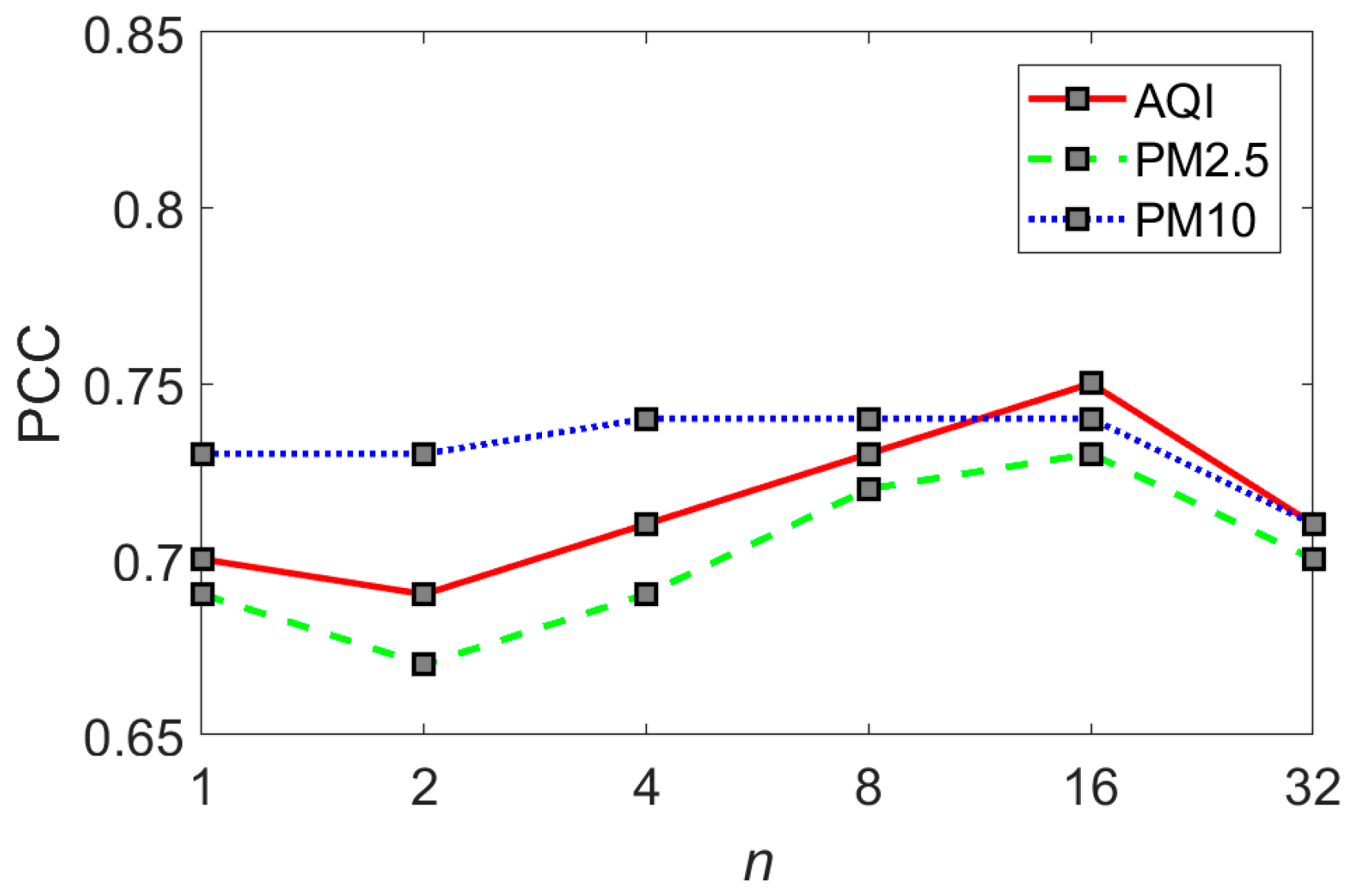
There are two parameters that need to be empirically determined in fastDBCP. The first is the down-sampling parameter n . The candidate should meet the requirements of delivering both a high correlation performance and real-time processing. To compare the influence of n , we sample the input hazy images to 1/ n of the original sizes to calculate their fastDBCP indexes. Then, the correlation coefficient between the objective index and the three air quality indicators, i.e., the AQI, PM2.5, and PM10, is calculated, respectively, and demonstrated in Figure 5.
The results in Figure 5 exceed our expectation. We find that the correlation between our visual indicator and the air quality indexes does not decrease with respect to the image size reduction. It is even better than that of the original size. This phenomenon applies for all the three air pollution indicators in the whole RHID_AQI dataset with cross-scene images. From Figure 5, we know that when an original 1177 × 786 image is scaled down 16 times, the correlation reaches its peak. Hence, the recommended image resolution for a reduced image I D would be around 48 × 48, in which case the output of the algorithm could reflect the level of air pollution best.
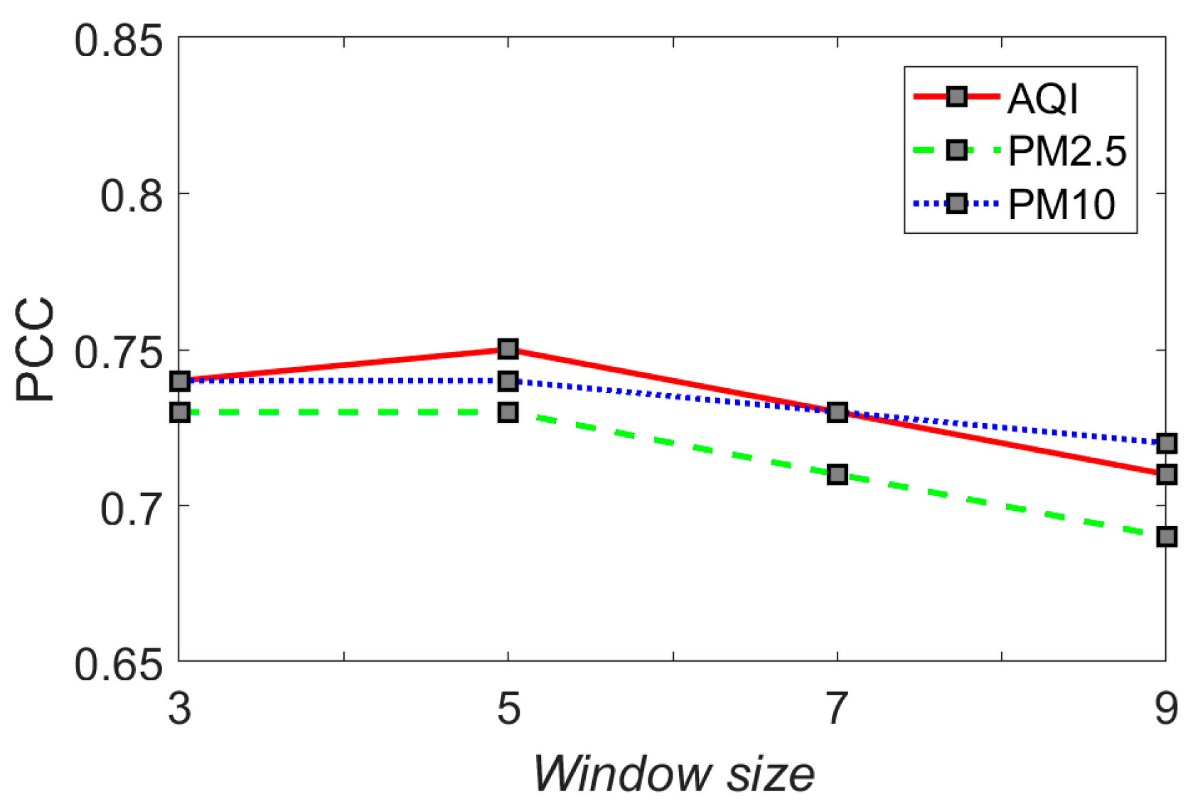
The second parameter needs to be determined is the size of the template window for dark channel prior and bright channel prior calculation in a single image. The effect of window size on haze level evaluations has been analyzed in [16], and the conclusion was that the performance is not sensitive to the variation in window size. However, for fastDBCP, the conclusion might be different. After the original image is scaled down, the window size should also be appropriately reduced to match it; additionally, this can save operation time. Here, we select different window sizes from 3 × 3 to 9 × 9 to observe the influence of this parameter in Figure 6, and suggest a window size of 5 × 5 due to its optimal performance.

3.2. Performance Comparison

We compute the correlation between visual indexes and air quality indicators, respectively, and list the results in Table 2. The visual indicators used for the comparison include subjective assessment scores provided by the RHID_AQI database, and a series of image quality evaluation indicators based on haze environment characteristics or deep learning. The results are satisfying. Some of the objective indicators even outperform the subjective MOS value. Among them, the deep learning method DIQaM-NR and our metric have an equally leading position. However, the proposed fastDBCP algorithm is better overall because it is much quicker, which will be demonstrated in the following section.

3.3. Computation Cost

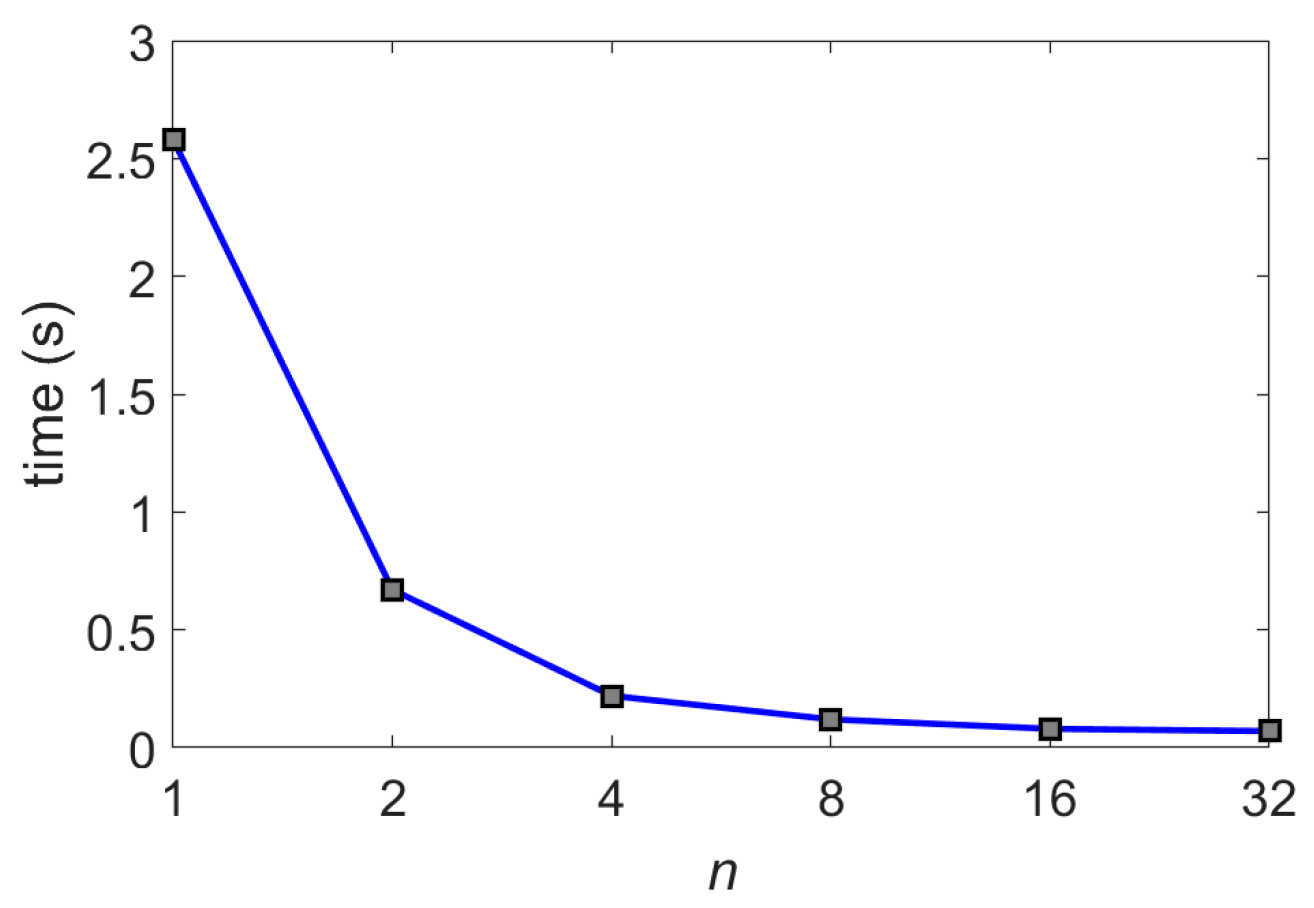
To further compare the computational cost, in Figure 7, we examine the average calculation time per image. As can be seen from the figure, the operation time decreases in an exponential trend. Taking n = 1 and n = 16 as an example, the processing time for each image is reduced from 2.58 s to 0.08 s, which means that the computational efficiency is 32 times better. This acceleration of speed is beneficial for an air quality real-time monitoring system. We also notice that the calculation speed in Figure 7 is not much different around n = 16 . Therefore, the size of the down-sampled image I D is suggested to be no smaller than 48 × 48 for both the performance and speed consideration.
Based on the performance of the objective metrics in Table 2, we choose relatively outstanding candidates to compare their computational speed. The configuration of our CPU computer is an Intel(R) Core (TM) i7-4790 CPU at 3.60 GHz with 12 GB RAM. The comparison results of the average computing time per image are shown in Table 3. It can be seen clearly that with the same performance, fastDBCP is ten times faster than the neighboring deep learning method.

4. Discussion

4.1. Application in Air Pollution Classfication

To further explore the potential of the proposed fastDBCP, we apply it to remote air pollution monitoring. So far, we have verified that the output of the metric can reflect the air pollution level visually in real-time. Furthermore, can we set a monitoring threshold so that when the real-time monitoring value falls below the threshold, the air pollution monitoring system will issue an alarm to alert the staff? The answer is yes. We take Beijing in the RHID_AQI database as an example and plot the calculated values of fastDBCP for each outdoor picture in Figure 8. The predicted air quality value for each image is displayed as a different shape and color, depending on its actual air pollution classification label. In addition, we calculate the optimal classification threshold and represent it by the horizontal demarcation line.
As can be seen from Figure 8, the distribution of the fastDBCP values is quite consistent with that of air pollution label. Except for one case, the pictures with unpolluted air quality are basically above the 0.59 demarcation line, while the pictures with polluted air quality are all below the threshold. The calculated threshold is helpful to group most of the data points into their own categories. For a quantitative illustration of this, the confusion matrixes are plotted in Figure 9, which shows that the proposed fastDBCP has good class spacing in its sample space and can segment the two types of the sample data in most cases.
To further compare the classification performance of different algorithms, we calculate the classification accuracy according to the following definition:
A c c = T P + T N P + N ,
where A c c represents the accuracy of classification, T P denotes the true positives, i.e., the number of unpolluted pictures that are correctly classified, T N denotes the true negatives, i.e., the number of polluted images that are correctly classified, and P and N are the number of pictures for the positive and negative samples, respectively.
So far, we know that the data calculated using fastDBCP have a clear class spacing and are easy to classify, but we do not know whether other indicators can obtain similarly good results. Therefore, we calculate the optimal threshold and corresponding classification accuracy of nine competing algorithms and list the results in Table 4. It can be seen that the fastDBCP method has a high classification accuracy and outperforms the other algorithms.

4.2. Application in Real-Time Monitoring System

The previous section mainly introduces the application of the proposed method in the field of air pollution monitoring. In fact, the fastDBCP approach has the potential to be applied to many more types of real-time monitoring systems. For example, in an autonomous driving scenario [39], it can effectively monitor the air quality of the current road surface. When hazy weather is a serious threat to driving safety, rapid warnings can be provided.
In addition, the fastDBCP index has a strong correlation with image visual quality reflecting the haziness degree in real environments, as shown in Table 5. According to the data in Table 3 and Table 5, the performance of the proposed fastDBCP is comparable to DBCP-II, DBCP-III, and the deep learning method DIQaM-NR, but has a ten-fold or greater advantage in terms of computing speed. This fast-processing capacity is a significant feature that enables it to be used in real-time monitoring systems. As shown in Figure 10, it can serve as a supplementary visual measure to detect other types of catastrophic weather having similar visual characteristics as hazy weather, such as forest fires [40], tornadoes [41], and so on. In these application scenarios, the speed of fastDBCP will be its advantage.

5. Conclusions

In this paper, we investigate an open question of whether we can sense air quality, especially the degree of air pollution, through visual information. After an analysis and verification, the following conclusions are obtained. First, the traditional image quality evaluation methods, especially the objective measurement index of image haze characteristics and deep learning methods, can reflect the air quality to a certain extent, with the same effect as the subjective index or even better. Second, the proposed air pollution evaluation method, i.e., fastDBCP, has a faster speed than the previous methods, and has a higher degree of correlation with the air quality indexes, so it can be applied to customized air pollution surveillance systems. Third, the presented novel metric could be integrated into an actual air pollution warning scheme to warn the aggravation of air pollution and could be used in hazy weather monitoring for automatic driving, tornado monitoring for weather forecasting, or forest fire predictions for disaster warnings.
Of course, our current research still has much room to improve. For example, fastDBCP cannot be compared and validated against other databases because we cannot find other publicly available datasets with both subjective measurements of images and air quality indicators. In addition, we hope to apply our indicators in a video surveillance system, but at present, there are few outdoor image and video quality evaluation databases for hazy weather [45], and no air quality indicator data are provided. Future studies should discover and build outdoor image or video databases that provide more accurate air quality indicators so that we can validate the performance of fastDBCP on these datasets and prove or verify the internal relationship between and mechanism of air quality and vision.

Author Contributions

Conceptualization, Y.C.; methodology, Y.C.; software, Y.C. and F.C.; validation, Y.C. and F.C.; formal analysis, Y.C. and H.F.; investigation, Y.C.; resources, Y.C.; data curation, Y.C.; writing—original draft preparation, Y.C.; writing—review and editing, H.F. and H.Y.; visualization, Y.C.; supervision, H.F. and H.Y.; project administration, Y.C.; funding acquisition, Y.C. All authors have read and agreed to the published version of the manuscript.

Funding

This research was funded by the Stabilization Support Plan for Shenzhen Higher Education Institutions, grant number 20200812165210001.

Data Availability Statement

The source codes are free to download from website: https://drive.google.com/file/d/1KW_WTZ-DpXIgCFDe_1B8mF4mHSkMHrrB/view?usp=sharing (accessed on 3 April 2023), or https://pan.baidu.com/s/1wLu1MxXor4FTFWBV99hfZw?pwd=DBCP with password DBCP (accessed on 3 April 2023).

Acknowledgments

We would like to thank the website siyuefeng.com, which held the public benefit photographic exhibition, i.e., “The breath of China”, in 2014, and thank the organizer and the photographers who authorized us to use the photos to build the RHID_AQI database. Specifically, we want to thank the following photographers who took the haze pictures: Yingjiu Zhao and Duona Fu in Beijing, Jianshi Zhou in Hangzhou, Hong Shu and Qing Xia in Kunming, Hao Luo and Dui Zha in Lasa, Xiaojun Guo and Bing Hu in Shijiazhuang, Jiang Liu in Taiyuan, Ye Xue and Xinjie Wu in Tianjin, and Xiaojuan Pan in Wuhan.

Conflicts of Interest

The authors declare no conflict of interest.

References

  1. Wong, C.J.; Matjafri, M.Z.; Abdullah, K.; Lim, H.S.; Low, K.L. Temporal air quality monitoring using surveillance camera. In Proceedings of the 2007 Geoscience and Remote Sensing Symposium, Barcelona, Spain, 23–28 July 2007; pp. 2864–2868. [Google Scholar] [CrossRef]
  2. Sallis, P.; Dannheim, C.; Icking, C.; Maeder, M. Air pollution and fog detection through vehicular sensors. In Proceedings of the 8th Asia Modelling Symposium, Taipei, Taiwan, 23–25 September 2014; pp. 181–186. [Google Scholar] [CrossRef]
  3. Mukundan, A.; Huang, C.C.; Men, T.C.; Lin, F.C.; Wang, H.C. Air pollution detection using a novel snap-shot hyperspectral imaging technique. Sensors 2022, 22, 6231. [Google Scholar] [CrossRef]
  4. Ma, K.; Liu, W.; Zhang, K.; Duanmu, Z.; Wang, Z.; Zuo, W. End-to-end blind image quality assessment using deep neural networks. IEEE Trans. Image Process. 2018, 27, 1202–1213. [Google Scholar] [CrossRef] [PubMed]
  5. Min, X.; Zhai, G.; Gu, K.; Yang, X.; Guan, X. Objective quality evaluation of dehazed images. IEEE Trans. Intell. Transp. Syst. 2019, 20, 2879–2892. [Google Scholar] [CrossRef]
  6. Li, B.; Ren, W.; Fu, D.; Tao, D.; Feng, D.; Zeng, W.; Wang, Z. Benchmarking single-image dehazing and beyond. IEEE Trans. Image Process. 2019, 28, 492–505. [Google Scholar] [CrossRef] [PubMed]
  7. Ancuti, C.O.; Ancuti, C.; Timofte, R. NH-HAZE: An image dehazing benchmark with non-homogeneous hazy and haze-free images. In Proceedings of the IEEE Computer Society Conference on Computer Vision and Pattern Recognition Workshops, Seattle, WA, USA, 14–19 June 2020; pp. 1798–1805. [Google Scholar] [CrossRef]
  8. Zhao, S.; Zhang, L.; Huang, S.; Shen, Y.; Zhao, S. Dehazing evaluation: Real-world benchmark datasets, criteria, and baselines. IEEE Trans. Image Process. 2020, 29, 6947–6962. [Google Scholar] [CrossRef]
  9. Sahu, G.; Seal, A.; Bhattacharjee, D.; Nasipuri, M.; Brida, P.; Krejcar, O. Trends and prospects of techniques for haze removal from degraded images: A survey. IEEE Trans. Emerg. Top. Comput. Intell. 2022, 6, 762–782. [Google Scholar] [CrossRef]
  10. Korhonen, J. Two-level approach for no-reference consumer video quality assessment. IEEE Trans. Image Process. 2019, 28, 5923–5938. [Google Scholar] [CrossRef]
  11. Tu, Z.; Wang, Y.; Birkbeck, N.; Adsumilli, B.; Bovik, A.C. UGC-VQA: Benchmarking blind video quality assessment for user generated content. IEEE Trans. Image Process. 2021, 30, 4449–4464. [Google Scholar] [CrossRef] [PubMed]
  12. Fu, X.; Lin, Q.; Guo, W.; Ding, X.; Huang, Y. Single image dehaze under non-uniform illumination using bright channel prior. J. Theor. Appl. Inf. Technol. 2013, 48, 1843–1848. [Google Scholar]
  13. Kang, L.; Ye, P.; Li, Y.; Doermann, D. Convolutional neural networks for no-reference image quality assessment. In Proceedings of the 2014 IEEE Conference on Computer Vision and Pattern Recognition, Columbus, OH, USA, 23–28 June 2014; pp. 1733–1740. [Google Scholar] [CrossRef]
  14. Choi, L.K.; You, J.; Bovik, A.C. Referenceless prediction of perceptual fog density and perceptual image defogging. IEEE Trans. Image Process. 2015, 24, 3888–3901. [Google Scholar] [CrossRef]
  15. Bosse, S.; Maniry, D.; Müller, K.R.; Wiegand, T.; Samek, W. Deep neural networks for no-reference and full-reference image quality assessment. IEEE Trans. Image Process. 2018, 27, 206–219. [Google Scholar] [CrossRef] [PubMed]
  16. Chu, Y.; Chen, F.; Fu, H.; Yu, H.Y. Haze level evaluation using dark and bright channel prior information. Atmosphere 2022, 13, 683. [Google Scholar] [CrossRef]
  17. Chu, Y.; Chen, Z.; Fu, Y.; Yu, H. Haze image database and preliminary assessments. In Proceedings of the Fully 3D Conference, San Diego, CA, USA, 18–23 June 2017; pp. 825–830. [Google Scholar]
  18. The Breath of China: Public-Benefit Exhibition. Available online: http://slide.news.sina.com.cn/x/slide_1_61471_68613.html/d/8#p=1 (accessed on 31 March 2023).
  19. Technical Regulation on Ambient Air Quality Index (on Trial). Available online: https://www.mee.gov.cn/ywgz/fgbz/bz/bzwb/jcffbz/201203/t20120302_224166.shtml (accessed on 3 April 2023).
  20. Final Report from the Video Quality Experts Group on the Validation of Objective Models of Video Quality Assessment—Phase II. Available online: http://www.vqeg.org (accessed on 31 March 2023).
  21. Pui, D.Y.H.; Chen, S.C.; Zuo, Z.L. PM2.5 in China: Measurements, sources, visibility and health effects, and mitigation. Particuology 2014, 13, 1–26. [Google Scholar] [CrossRef]
  22. Oliveira, M.; Slezakova, K.; Delerue-Matos, C.; Pereira, M.C.; Morais, S. Children environmental exposure to particulate matter and polycyclic aromatic hydrocarbons and biomonitoring in school environments: A review on indoor and outdoor exposure levels, major sources and health impacts. Environ. Int. 2019, 124, 180–204. [Google Scholar] [CrossRef] [PubMed]
  23. Wang, Z.; Bovik, A.C.; Sheikh, H.R.; Simoncelli, E.P. Image quality assessment: From error visibility to structural similarity. IEEE Trans. Image Process. 2004, 13, 600–612. [Google Scholar] [CrossRef] [PubMed]
  24. Saad, M.A.; Bovik, A.C.; Charrier, C. Blind image quality assessment: A natural scene statistics approach in the DCT domain. IEEE Trans. Image Process. 2012, 21, 3339–3352. [Google Scholar] [CrossRef] [PubMed]
  25. Xue, W.; Mou, X.; Zhang, L.; Bovik, A.C.; Feng, X. Blind image quality assessment using joint statistics of gradient magnitude and Laplacian features. IEEE Trans. Image Process. 2014, 23, 4850–4862. [Google Scholar] [CrossRef]
  26. Mittal, A.; Moorthy, A.K.; Bovik, A.C. No-reference image quality assessment in the spatial domain. IEEE Trans. Image Process. 2012, 21, 4695–4708. [Google Scholar] [CrossRef]
  27. Chu, Y.; Mou, X.; Fu, H.; Ji, Z. Blind image quality assessment using statistical independence in the divisive normalization transform domain. J. Electron. Imaging 2015, 24, 063008. [Google Scholar] [CrossRef]
  28. Moorthy, A.K.; Bovik, A.C. A two-step framework for constructing blind image qualityindices. IEEE Signal Process. Lett. 2010, 17, 513–516. [Google Scholar] [CrossRef]
  29. Liu, L.; Dong, H.; Huang, H.; Bovik, A.C. No-reference image quality assessment in curvelet domain. Signal Process. Image Commun. 2014, 29, 494–505. [Google Scholar] [CrossRef]
  30. Moorthy, A.K.; Bovik, A.C. Blind image quality assessment: From natural scene statistics to perceptual quality. IEEE Trans. Image Process. 2011, 20, 3350–3364. [Google Scholar] [CrossRef] [PubMed]
  31. He, K.; Sun, J.; Tang, X. Single image haze removal using dark channel prior. IEEE Trans. Pattern Anal. Mach. Intell. 2011, 33, 2341–2353. [Google Scholar] [CrossRef]
  32. Wang, Y.T.; Zhuo, S.J.; Tao, D.P.; Bu, J.J.; Li, N. Automatic local exposure correction using bright channel prior for under-exposed images. Signal Process. 2013, 93, 3227–3238. [Google Scholar] [CrossRef]
  33. He, K.; Sun, J.; Tang, X. Guided image filtering. IEEE Trans. Pattern Anal. Mach. Intell. 2013, 35, 1397–1409. [Google Scholar] [CrossRef]
  34. Otsu, N. A threshold selection method from gray-level histograms. IEEE Trans. Syst. Man Cybern. 1979, 9, 62–66. [Google Scholar] [CrossRef]
  35. Zhan, Y.; Zhang, R.; Wu, Q.; Wu, Y. A new haze image database with detailed air quality information and a novel no-reference image quality assessment method for haze images. In Proceedings of the 2016 IEEE International Conference on Acoustics, Speech and Signal Processing, Shanghai, China, 20–25 March 2016; pp. 1095–1099. [Google Scholar] [CrossRef]
  36. Li, Y.; Huang, J.; Luo, J. Using user generated online photos to estimate and monitor air pollution in major cities. In Proceedings of the 7th International Conference on Internet Multimedia Computing and Service, Zhangjiajie, China, 19–21 August 2015; pp. 11–15. [Google Scholar] [CrossRef]
  37. Hsieh, C.H.; Horng, S.C.; Huang, Z.J.; Zhao, Q. Objective haze removal assessment based on two-objective optimization. In Proceedings of the IEEE 8th International Conference on Awareness Science and Technology, Taichung, Taiwan, 8–10 November 2017; pp. 279–283. [Google Scholar] [CrossRef]
  38. Lu, H.; Zhao, Y.; Zhao, Y.; Wen, S.; Ma, J.; Keung, L.H.; Wang, H. Image defogging based on combination of image bright and dark channels. Guangxue Xuebao/Acta Opt. Sin. 2018, 38, 1115004. [Google Scholar] [CrossRef]
  39. Johari, A.; Swami, P.D. Comparison of autonomy and study of deep learning tools for object detection in autonomous self driving vehicles. In Proceedings of the 2nd International Conference on Data, Engineering and Applications, Bhopal, India, 28–29 February 2020; pp. 1–6. [Google Scholar] [CrossRef]
  40. Ichoku, C.; Kaufman, Y.J. A method to derive smoke emission rates from MODIS fire radiative energy measurements. IEEE Trans. Geosci. Remote Sens. 2005, 43, 2636–2649. [Google Scholar] [CrossRef]
  41. Jun, L.; Honggen, Z.; Jianbing, L.; Xinan, L. Research on the networking strategy of tornado observation network in northern Jiangsu based on X-band weather radar. In Proceedings of the 2019 International Conference on Meteorology Observations, Chengdu, China, 28–31 December 2019; pp. 1–4. [Google Scholar] [CrossRef]
  42. Smog in Beijing. Available online: http://www.cd-pa.com/bbs/thread-572953-1-1.html (accessed on 1 April 2023).
  43. Forest Fire in Xichang. Available online: https://sputniknews.cn/20200331/1031118848.html (accessed on 1 April 2023).
  44. High-Definition Tornado Pictures. Available online: https://www.jj20.com/tp/242085.html (accessed on 1 April 2023).
  45. Chu, Y.; Luo, G.; Chen, F. A real haze video database for haze level evaluation. In Proceedings of the 13th International Conference on Quality of Multimedia Experience, Montreal, QC, Canada, 14–17 June 2021; pp. 69–72. [Google Scholar] [CrossRef]
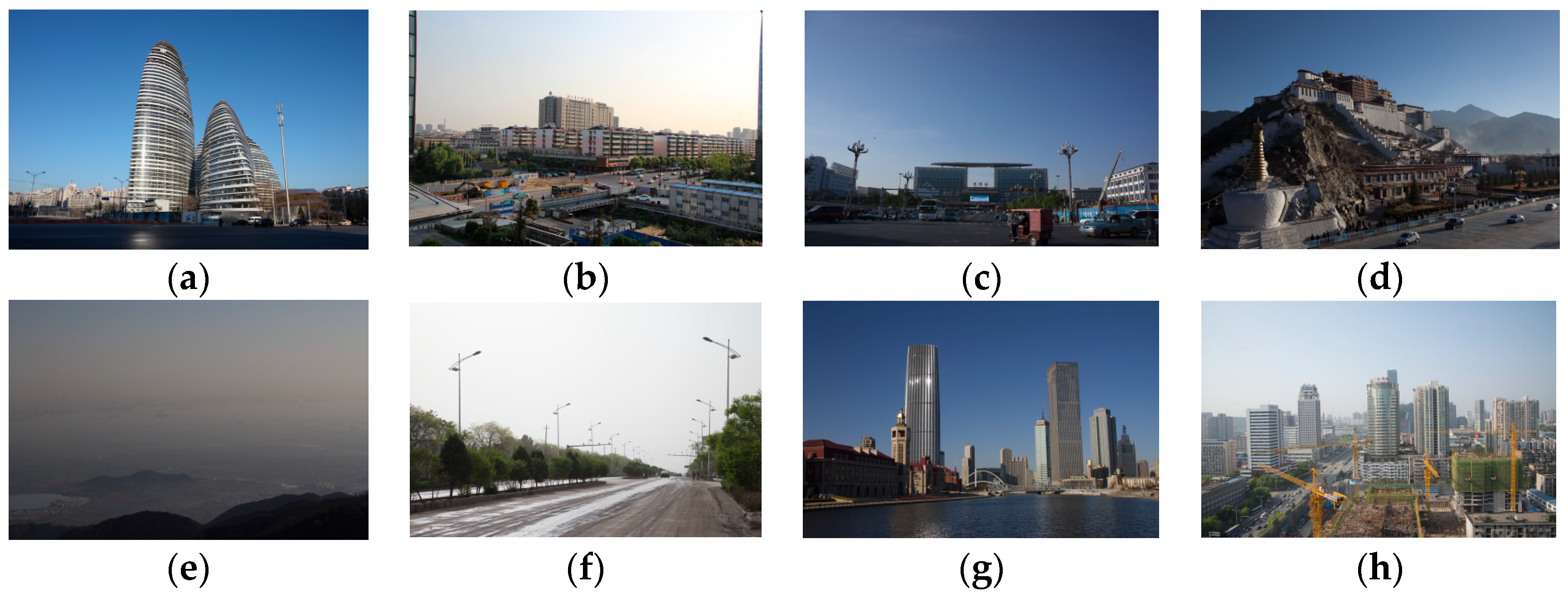
Figure 1. Representative image of each environment in the RHID_AQI dataset. (a) Beijing; (b) Hangzhou; (c) Kunming; (d) Lasa; (e) Shijiazhuang; (f) Taiyuan; (g) Tianjin; and (h) Wuhan.
Atmosphere 14 00772 g001
Figure 2. Variation tendency of subjective scores and environmental indexes for six pictures with different levels of air pollution. (a) MOS values; (b) AQI values; (c) PM2.5 values; (d) PM10 values.
Atmosphere 14 00772 g002
Figure 3. Scatter plots of MOS values vs. environmental indexes for an environment in Beijing in the RHID_AQI database. (a) AQI, PCC = −0.85; (b) PM2.5, PCC = −0.89; (c) PM10, PCC = −0.67.
Atmosphere 14 00772 g003
Figure 4. Illustration of the insensitive property of C db . (a) the original and reduced images. (b) the corresponding C db in different scales. (c) the histogram and segmentation threshold of the corresponding C db .
Atmosphere 14 00772 g004
Figure 5. Comparison of the influence of down-sampling parameter on correlation results.
Atmosphere 14 00772 g005
Figure 6. Comparison of the correlation results with respect to different window sizes.
Atmosphere 14 00772 g006
Figure 7. Comparison of computation cost using down-sampling strategy.
Atmosphere 14 00772 g007
Figure 8. Illustration of the classification for unpolluted and polluted weather in Beijing using fastDBCP as indicator.
Atmosphere 14 00772 g008
Figure 9. Confusion matrix for haze category classifiers.
Atmosphere 14 00772 g009
Figure 10. Typical pictures of pollution weather: (a) heavy haze [42]; (b) forest fire smoke [43]; (c) tornado [44].
Atmosphere 14 00772 g010
Table 1. AQI and air pollution category in the RHID_AQI dataset.
AQIAir Pollution LevelAir Pollution CategoryClassification LabelClassification Category
0–501good0unpolluted
51–1002moderate0unpolluted
101–1503lightly polluted1polluted
151–2004moderately polluted1polluted
201–3005heavily polluted1polluted
>3006severely polluted1polluted
Table 2. Comparison of PCC between visual indexes and air pollution indicators on the RHID_AQI dataset.
MethodAQIPM2.5PM10
MOS0.71 0.70 0.70
R [35]0.68 0.66 0.71
t ¯ [36]0.32 0.36 0.30
C [12]0.68 0.66 0.74
μ [37]0.34 0.36 0.30
A v e r a g e [38]0.19 0.09 0.31
V a r i a n c e [38]0.53 0.48 0.60
E n t r o p y [38]0.64 0.62 0.67
D [14]0.65 0.64 0.71
DBCP-I [16]0.68 0.66 0.73
DBCP-II [16]0.69 0.68 0.72
DBCP-III [16]0.71 0.69 0.75
CNN [13]0.68 0.66 0.72
DIQaM-NR [15]0.750.72 0.75
fastDBCP0.750.730.74
Table 3. Comparison of computation cost among different image quality evaluation metrics on the RHID_AQI dataset.
Method R C E n t r o p y D DBCP-IDBCP-IIDBCP-IIICNNDIQaM-NRfastDBCP
Computation time (s)1.340.070.021.862.791.542.800.330.810.08
Table 4. Comparison of classification accuracy among different image quality evaluation metrics on the RHID_AQI dataset.
Method R C E n t r o p y D DBCP-IDBCP-IIDBCP-IIICNNDIQaM-NRfastDBCP
A c c (%)78.7475.4277.7454.4977.7479.4081.0654.4954.4982.39
Table 5. Comparison of PCC between different image quality indexes and subjective scores on the RHID_AQI dataset.
Method R C E n t r o p y D DBCP-IDBCP-IIDBCP-IIICNNDIQaM-NRfastDBCP
PCC0.790.810.700.820.880.930.920.850.930.91
Disclaimer/Publisher’s Note: The statements, opinions and data contained in all publications are solely those of the individual author(s) and contributor(s) and not of MDPI and/or the editor(s). MDPI and/or the editor(s) disclaim responsibility for any injury to people or property resulting from any ideas, methods, instructions or products referred to in the content.