The Role of Neutral Wind Velocity and Its Vertical Component on Predictability of Formation and Localization of Sporadic E (Es)

Abstract

The formation and localization of sporadic E (Es) layers predicted by the ion vertical drift velocity and its vertical change in the lower thermosphere during nighttime are shown analytically and by numerical simulations. The consideration of the existence of a minimum negative value of the vertical change of the ion vertical drift velocity as a necessary condition of formation of the Es layer and determining ion convergence rate into this layer is extended in case of the presence of vertical wind. Upward vertical wind can shift the convergence regions upward, while downward vertical wind shifts them downward, unlike the cases of the presence of only meridional and zonal winds. It also changes the ion convergence rate compared to the one with just a horizontal wind. It is shown for the first time that the upward constant wind also causes the convergence of ions with the maximum rate in the region where the ion-neutral collision frequency is equal to their cyclotron frequency. While demonstrating the presented theory by numerical simulations, HWM14 data is used for the meridional and zonal wind velocity profiles and the presence of its vertical component is assumed. In this case, in addition to the estimated ion drift velocity and its vertical changes, their initial distribution and ambipolar diffusion also determine the development of ion convergence/divergence processes. For a small magnitude of vertical wind velocity, its significant influence on the ions/electrons behavior is demonstrated, which shows the importance of both tidal wind and wind changes caused by the propagation of atmospheric gravity waves on the formation of the Es layer. In this theoretical research, it is shown that the realistic profile of the wind velocity, which takes into account the vertical component along with its zonal and meridional ones, is important for the prediction of the Es layers formation, as well as regions of ion depletion.

1. Introduction

Sporadic E (Es) is a high-density narrow and irregular ionosphere layer [1,2], and its existence was noticed in the ionograms of 1933–1935 [3]. In this layer, the ion/electron density can be comparable to or greater than those of the regular ionosphere E, F1 and F2 layers. Therefore, Es may influence the quality of radio communications [4,5].

Es layers occur during nighttime and more frequently during daytime in the lower thermosphere, at altitudes between 90–150 km [3,6,7]. This fact indicates that in this range of altitudes, the conditions for ion/electron convergence into a narrow layer are provided [8,9,10,11,12,13,14]. This convergence and, consequently, the formation of the Es layer can be caused by the horizontal wind with vertical shear (windshear theory) [8,9,15,16,17,18,19,20], by an electric field and its variations [21,22] and/or by the combined action of all these effects [23,24,25]. By using the set of magnetohydrodynamic equations for the mid-latitude lower thermosphere, the ion vertical drift velocity can be estimated by the wind velocity, the vertical distribution of this region’s dominant neutral particles and the geomagnetic field. By this drift velocity and its vertical changes, the height regions can be estimated where the ion/electron convergence or depletion occurs [12,14,26]. The loss rate of molecular ions (e.g., NO⁺ and O²⁺) increases during ion/electron convergence into a thin dense layer, which in turn causes the dominance of long-lived heavy metallic ions (e.g., Fe⁺ and Mg⁺), which is a phenomenon that has been observed in nighttime Es layers [27,28].

In recent studies [12,26] it was shown that in addition to earlier considerations [2,3,15,29,30], which took into account the “windshear” effect, the wind magnitude and direction were important for the development of ion/electron convergence (or divergence/depletion) in certain height regions. It was also shown that Es layer density is controlled by ion ambipolar diffusion as well.

In the present study, the suggested theoretical mechanism of the Es layer formation takes into account an arbitrary wind height profile. This approach is different from the earlier considerations [12,26]. In this study, the recently obtained results of the case of horizontal wind are also generalized. This makes the formation of the Es layers more predictable. These processes can also be described by an analytical approach. The behavior of the vertical distribution of ion density $N_i(z,t)$ in an ambipolar approach and correspondingly the formation of ionosphere layers, similar to [12,26,31] (with some extension, including gravity effect as well), can be described by the following equation:

$$\frac{\partial N_i}{\partial t}=-\frac{\partial {\mathrm{w}}_{i\mathrm{v}}}{\partial z}{N}_i-{\mathrm{w}}_{i\mathrm{v}}(z)\frac{\partial N_i}{\partial z}+\frac{\partial }{\partial z}{D}_a(z)\left(\frac{\partial N_i}{\partial z}+\frac{N_i}{H_i}\right)+Q-L$$

(1)

Here, in the expression of ion vertical drift velocity ${\mathrm{w}}_i$, the ${\mathrm{w}}_{i\mathrm{v}}$ part caused by neutral wind and the part $-D_a(z)\left(\frac{\partial N_i}{\partial z}+\frac{N_i}{H_i}\right)$ caused by ions ambipolar diffusion ($\propto D_a$) are separated. This separation makes further analysis more convenient. $D_a$ is the coefficient of ion ambipolar diffusion. Q and L are the ion production and loss rates, respectively. $H_i$ is the ion scale height. The effect of gravity in the lower thermosphere (h < 140 km) is relatively small ($\left|\frac{\partial N_i}{\partial z}\right|>>\frac{N_i}{H_i}$). Here and hereafter, the vertical coordinate z represents the residual between some actual $h$ and initial heights $h_o$ ($z=h-h_o$).

Despite the fact that ionosphere plasma is weakly ionized and the influence of neutrals on the ion/electron drift velocity and correspondingly on their density behavior is important, the formation of the regular ionosphere E, F1 and F2 layers is still possible, even in the absence of neutral wind ($V=0$ and ${\mathrm{w}}_{i\mathrm{v}}=0$). For example, in the lower thermosphere, the formation of the E layer by the Chapman mechanism is mainly determined by the photoionization rate ($Q$) of molecules (e.g., O₂ and N₂) with vertically decreasing density [5].

For the formation of the F1 layer during daytime (mostly in the summer season, at a height of about 180–250 km), the photoionization of atomic oxygen is important, which decreases in density with height, since the electron production is dominated by extreme ultraviolet (UV, 10–100 nm) radiation ionizing atomic oxygen. During the night, the photoionization is absent ($Q=0$), so the F1 layer vanishes, and the F2 becomes a dominant layer. This layer regularly exists (with peak electron density at about 300–400 km height) and it is maintained by the increase in ion ambipolar diffusion displacement ($-D_a(z)\left(\frac{\partial N_i}{\partial z}+\frac{N_i}{H_i}\right)$) above the electron density peak height [5]), as well as by the increase in ion recombination below this height. Here, these processes are slower than in the E and F1 regions, allowing the F2 layer to exist during both daytime, when photoionization increases ($Q>0$), and nighttime, when ionization is absent ($Q=0$). Although the neutral wind is not necessary for the formation of the E, F1 and F2 layers, it can significantly influence ion/electron vertical drift described by ${\mathrm{w}}_{i\mathrm{v}}$, as in Equation (1), and therefore affect the behavior of these layers.

In the suggested study, unlike the regular ionosphere E, F1 and F2 layers, the formation of the sporadic E (Es) layer at mid-latitude lower thermosphere is mainly determined by the neutral wind. The ion vertical drift velocity, caused by the combined effect of vertically changing ion-neutral collision and Lorentz forcing, changes during the existence of homogeneous or inhomogeneous wind ($\frac{\partial {\mathrm{w}}_{i\mathrm{v}}}{\partial z}\ne 0$). At some height regions, this drift velocity is zero (${\mathrm{w}}_{i\mathrm{v}}=0$), depending on the direction of the wind. These height regions ${\mathrm{w}}_{i\mathrm{v}}=0$ will be noted as a node of ion drift velocity. When the ion upstream and downstream flows ($(div\mathbf{w}\approx \frac{\partial {\mathrm{w}}_{i\mathrm{v}}}{\partial z})\min <0$) towards this region occur, then their convergence into a thin Es-type layer is possible at this node [26]. The processes of ions convergence into a thin layer should take place until the increase in the density due to the convergence exceeds its decrease due to diffusive displacement ($\propto D_a$), and total loss ($Q-L<0$) caused by their production ($Q$) and loss ($L$) rates.

For those wind directions when the ions downstream and upstream flows occur ($(div\mathbf{w}\approx \frac{\partial {\mathrm{w}}_{i\mathrm{v}}}{\partial z})\max >0$), the opposite phenomenon takes place in these height regions—the ion/electron depletion. Further, we will show that both horizontal and vertical components of the wind velocity are important for the estimation of the ion/electron convergence/divergence regions and prediction of the development of corresponding processes.

To show the suggested theoretical mechanism of sporadic E formation, we will solve Equation (1) using an analytic approach when

$$-\frac{\partial {\mathrm{w}}_{i\mathrm{v}}}{\partial z}\equiv C^{\prime }=constant$$

(2)

and $D_a=const$. In this case, the solution of Equation (1) has the following form:

$$N_i(z,t)=\frac{e^{C\prime (t-t_o)}}{2{[\pi D_a(t-t_o)]}^{1/2}}{\displaystyle \underset{-\infty }{\overset{+\infty }{\int }}{e}^{-\frac{{[z-{\mathrm{w}}_{i\mathrm{v}}(t-t_o)-z^{\prime }]}^2}{4D_a(t-t_o)}}{N}_{io}(z^{\prime })d{z}^{\prime }}$$

(3)

Here,

$$G_i(z,t)=\frac{e^{C^{\prime }(t-t_o)}}{2{[\pi D_a(t-t_o)]}^{1/2}}{e}^{-\frac{{[z-{\mathrm{w}}_{i\mathrm{v}}(t-t_o){}^{\prime }]}^2}{4D_a(t-t_o)}}$$

(4)

is the analogy of the source function [32], which corresponds to the solution of Equation (1) in the case of $Q-L=0$. When $C^{\prime }>0$, then $G_i(z,t)$ increases with time, and when $C^{\prime }<0$, it decreases. Equation (3) also shows that for ion vertical drift velocity ${\mathrm{w}}_{i\mathrm{v}}>0$, the initial peak height $z_m(t=t_o)=0$ of $G_i(z,t)$ shifts upward and for ${\mathrm{w}}_{i\mathrm{v}}<0$ it descends. We note that the upward shift of the ion’s initial layer, ${\mathrm{w}}_{i\mathrm{v}}$, is not noticeable when ion diffusion is neglected.

In Equation (3), the value $\propto {\displaystyle \underset{-\infty }{\overset{+\infty }{\int }}{e}^{-\frac{{[z-{\mathrm{w}}_{i\mathrm{v}}(t-t_o)-z^{\prime }]}^2}{4D_a(t-t_o)}}{N}_{io}(z^{\prime })d{z}^{\prime }}$ indicates that, in addition to the diffusive displacement of the ion’s initial distribution $N_{io}(z)$, their redistribution also occurs in the height region of its drift velocity node, ${\mathrm{w}}_{i\mathrm{v}}=0$.

When the increase in ions density ($\propto e^{C\prime (t-t_o)}>1$), caused by vertical changes of ion vertical drift velocity ($C^{\prime }>0$), exceeds the diffusive displacement of their initial density ($\propto {\displaystyle \underset{-\infty }{\overset{+\infty }{\int }}{e}^{-\frac{{[z-{\mathrm{w}}_{i\mathrm{v}}(t-t_o)-z^{\prime }]}^2}{4D_a(t-t_o)}}{N}_{io}(z^{\prime })d{z}^{\prime }}$), then the density in the layers formed in the nodes increases; see Equation (3). Equation (3) also shows that when $C^{\prime }<0$ and, correspondingly, $e^{C\prime (t-t_o)}<1$, then in this region the opposite phenomenon takes place—its density decreases (depletes).

Actually, $C^{\prime }=-\frac{\partial {\mathrm{w}}_{i\mathrm{v}}}{\partial z}$ changes with height and their influence on ion/electron density variations will differ across various height regions. If a certain height $C^{\prime }$ has a maximal positive value ($C_{\max }^{\prime }>0$), then, considering ion/electron density behavior approximation by Equation (3), ions/electrons will be accumulated into a thin layer in the vicinity of this height, and the Es-type layer formation is expectable.

Here and hereafter, the superscript prime denotes the vertical derivative of the corresponding function, and the subscript max or min denotes its minimum and maximum values, respectively.

Using the approximated value of ${\mathrm{w}}_{i\mathrm{v}}(z)$ at the region $z=z_o$, it can be shown that

$${\mathrm{w}}_{i\mathrm{v}}\approx {\mathrm{w}}_{i\mathrm{v}}(z=z_o)+(z-z_o){\left(\frac{\partial {\mathrm{w}}_{i\mathrm{v}}}{\partial z}\right)}_{z=z_o}+\frac{1}{2}{(z-z_o)}^2{\left(\frac{{\partial }^2{\mathrm{w}}_{i\mathrm{v}}}{\partial z^2}\right)}_{z=z_o}$$

(5)

where $C^{\prime }=-{\left(\frac{\partial {\mathrm{w}}_{i\mathrm{v}}}{\partial z}\right)}_{z=z_o}$ is maximal ($C_{\max }^{\prime }>0$) or minimal ($C_{\min }^{\prime }<0$), then ${\left(\frac{{\partial }^2{\mathrm{w}}_{i\mathrm{v}}}{\partial z^2}\right)}_{z=z_o}=0$.

Equations (2)–(5) show that when $C_{\max }^{\prime }>0$, then the ions flow upstream ${\left(N_i{\mathrm{w}}_{i\mathrm{v}}\right)}_{z<z_o}\propto (z-z_o){\left(\frac{\partial {\mathrm{w}}_{i\mathrm{v}}}{\partial z}\right)}_{z=z_o}>0$ and downstream ${\left(N_i{\mathrm{w}}_{i\mathrm{v}}\right)}_{z>z_o}\propto (z-z_o){\left(\frac{\partial {\mathrm{w}}_{i\mathrm{v}}}{\partial z}\right)}_{z=z_o}<0$ to the region $z=z_o$, where their density increases maximally ($\propto \exp [C^{\prime }(t-t_o)]>1$), as in Equations (3) and (4). So, the formation of a high-density Es-type narrow layer occurs at the region of the ion vertical drift velocity node $z=z_o$ (${\mathrm{w}}_{i\mathrm{v}}=0$).

We note that this process can be developing along with the vertical drift of ions, during which the formed layer moves or is localized in the region where ${\mathrm{w}}_{i\mathrm{v}}\to 0$. If the height region with ${\mathrm{w}}_{i\mathrm{v}}=0$ is shifted from the region with $C^{\prime }>0$, then, according to Equations (3) and (4), the ion vertical convergence at this region is expectable during ions’ upward (${\mathrm{w}}_{i\mathrm{v}}(z=z_o>z_c)>0$) or downward (${\mathrm{w}}_{i\mathrm{v}}(z=z_o>z_c)<0$) drift. Equation (4) also shows that when $C^{\prime }<0$, then at the $z=z_o$ region, the opposite effect occurs: the ions downstream ${\left(N_i{\mathrm{w}}_{i\mathrm{v}}\right)}_{z<z_o}\propto (z-z_o){\left(\frac{\partial {\mathrm{w}}_{i\mathrm{v}}}{\partial z}\right)}_{z=z_o}<0$ and upstream ${\left(N_i{\mathrm{w}}_{i\mathrm{v}}\right)}_{z>z_o}\propto (z-z_o){\left(\frac{\partial {\mathrm{w}}_{i\mathrm{v}}}{\partial z}\right)}_{z=z_o}>0$ flows increase, resulting in the depletion of ions density at regions with $C_{\min }^{\prime }<0$, as in Equations (4) and (5).

We note that, for certain directions of the horizontal wind, vertical changes of the ion vertical drift velocity already have minimal negative ($C_{\max }^{\prime }>0$) or/and maximal positive ($C_{\min }^{\prime }<0$) values, even if the wind is homogeneous [12]. Therefore, at height ranges of 90–150 km, the processes of ions convergence into a thin layer or their depletion are possible. The formation of the Es-type layer (at a region with ${\mathrm{w}}_{i\mathrm{v}}=0$) occurs until its density increase is balanced by the increased ions diffusive outflow from this layer ($e^{C\prime (t-t_o)}=\frac{1}{2{[\pi D_a(t-t_o)]}^{1/2}}{\displaystyle \underset{-\infty }{\overset{+\infty }{\int }}{e}^{-\frac{{[z-{\mathrm{w}}_{i\mathrm{v}}(t-t_o)-z^{\prime }]}^2}{4D_a(t-t_o)}}{N}_{io}(z^{\prime })d{z}^{\prime }}$).

It is also important to note that heavy ions are mainly distributed between about 90–150 km [33,34] and correspondingly the increase in density of the Es layer continues during its upward ${\mathrm{w}}_{i\mathrm{v}}\to +0$ (towards the topside) or downward ${\mathrm{w}}_{i\mathrm{v}}\to -0$ (towards the bottom) motions where vertical changes of the vertical drift velocity vanish ($\frac{\partial {\mathrm{w}}_{i\mathrm{v}}}{\partial z}\to 0$).

The wind in the lower thermosphere can be caused by vertically propagating tidal motion, planetary waves and/or atmospheric gravity waves (AGWs). In this case, the ion vertical drift velocity can have several nodes where the ions’ convergence (when $C_{\max }^{\prime }>0$) or divergence (when $C_{\min }^{\prime }<0$) is possible. So, during the presence of more than one node with the condition $C_{\max }^{\prime }>0$, the formation of multilayered sporadic E is expectable [26].

So, on the basis of the realistic height profile of the neutral wind velocity and the ions’ initial distribution, the prediction of the formation of the Es-layer in the mid-latitude lower thermosphere is possible. Under the same conditions, the estimation of the ions depletion region is also possible. In these cases, both horizontal and vertical components of the wind profile are important, which will be shown in the suggested study.

Hereafter, for demonstration of the above-derived analytical theory of the formation of sporadic E and ions density depletion under the influence of neutral wind, we will solve Equation (1) numerically. In the equation for ions’ vertical drift velocity, ${\mathrm{w}}_i$ the neutral wind effect (${\mathrm{w}}_{i\mathrm{v}}$) will be distinguished from its drift by ions’ ambipolar diffusion. The convergence/divergence rate parameter $-\frac{\partial {\mathrm{w}}_{i\mathrm{v}}}{\partial z}\equiv C^{\prime }=constant$ will be generalized for a variable wind velocity profile and the equations describing the role of (1) its magnitude and direction, (2) the vertical changes of the horizontal components, and (3) the vertical changes of the vertical component will be separated. Unlike earlier considerations [12], the influence of vertical wind on both the convergence of ions and their depletion in a region of a certain height of the lower thermosphere will be shown.

In the first stage, we show only the effect of vertical wind on the convergence/divergence of ions. Further, we will consider its existence in the horizontal wind, whose meridional and zonal velocity profiles are determined by HWM14 data [35]. As an example, in numerical simulations, we use the HWM14 data for the mid-latitude (45° ± 2° N, 45° ± 2° E) lower thermosphere region at nighttime (from LT 23:00) around the spring equinox (e.g., day 102).

We will choose a small magnitude of vertical wind velocity, which can be caused by both tidal motions and AGWs often observed in the lower thermosphere [36,37]. We will show its influence on the location of the Es layer (e.g., the location with ${\mathrm{w}}_{i\mathrm{v}}=0$ or ${\mathrm{w}}_{i\mathrm{v}}\to 0$), as well as the presence of convergence (with $\left(\partial {\mathrm{w}}_{i\mathrm{v}}/\partial z\right)\min <0$) and divergence (with $\left(\partial {\mathrm{w}}_{i\mathrm{v}}/\partial z\right)\max >0$) height regions, and the development of corresponding ion/electrons density convergence/depletion processes in these regions. For the considered wind velocity profiles, the location of the height regions of maximum convergence and divergence rates, as well as the parameters caused by the magnitude, direction and vertical change of the wind, will be demonstrated. Theoretical and corresponding numerical simulations show that in the mid-latitude regions the formation of the sporadic E (Es), along with the significant effect of vertical shear of the horizontal wind (shear theory) [38,39], the factor of the magnitude and direction of the three-dimensional wind is important.

Sporadic E contains mainly metallic ions and, consequently, it is important to know the realistic wind velocity height profile, to study their global and regional distributions.

2. Parameters Describing the Formation of Sporadic E under the Influence of Neutral Wind

In this section, we consider the behavior of ions/electrons and the possibility of sporadic E formation in the mid-latitude lower thermosphere under the influence of arbitrarily directed neutral wind.

In this case, we use Equation (1) to study the behavior of heavy metallic ions (Fe⁺) and electrons under the assumption of quasi-neutrality ($N_i=N_e$), where the ions’ vertical drift velocity ${\mathrm{w}}_{i\mathrm{v}}$ (determined by the wind) and their vertical changes $\frac{\partial {\mathrm{w}}_{i\mathrm{v}}}{\partial z}$ vary in time. Here, along with the effect of wind shear, the influence of its magnitude and direction on the process of ions/electrons convergence into a narrow Es-type layer (convergence instability) and the importance of balancing this convergence by ambipolar diffusion will be taken into account. We also solve the ion/electron continuity equation with an analytical approach, which, similar to Equations (2)–(4), shows the formation of the Es layer and the tendency for its localization in the region of nodes of ion drift velocity ${\mathrm{w}}_{i\mathrm{v}}$. We use the analytical profiles of ion/electron density to set initial conditions, and then solve their basic equation, which takes into account the presence of wind with arbitrary direction, using numerical methods in the following cases: (1) in the presence of vertical wind only; (2) in the presence of horizontal wind whose meridional and zonal components are determined by HWM14 data; and (3) in the presence of wind determined by the above-mentioned vertical and zonal components. In these cases, the process of formation and localization of the Es layer throughout the night (covering 12-h intervals) will be shown. Assuming the presence of a vertical wind component, we demonstrate its significant influence on the formation and localization of the Es layer. The demonstrated numerical results align with its analytically predicted behavior. Additionally, we will show the impact of vertical wind on the ion/electron depletion process.

The neutral particles with velocity $V(V_x,V_y V_z)$ in the lower thermosphere influence the ion vertical drift via the combined action of the Lorentz forcing and ion-neutral collision. We take a right-handed set of coordinates (x, y, z) with x directed to the magnetic north, y to the west and z vertically upward. In this case, the dependence of the ions’ vertical drift velocity ${\mathrm{w}}_i$ on the neutral wind velocity, taking into account their ambipolar diffusion ($\propto D_a$), can be described by the equation [22,29,30]:

$${\mathrm{w}}_i={\mathrm{w}}_{i\mathrm{v}}-D_a(z)\frac{1}{N_i}\frac{\partial N_i}{\partial z}$$

(6)

where the influence of neutral wind velocity $V(V_x,V_y V_z)$ on the ion vertical drift velocity ${\mathrm{w}}_i$ is considered in the value of ${\mathrm{w}}_{i\mathrm{v}}$, which has the following form [2,23,30]:

$${\mathrm{w}}_{i\mathrm{v}}(z,t)=-C_x(z)V_x(z,t)-C_y(z)V_y(z,t)+C_z(z)V_z(z,t)$$

(7)

Here, considerations of the recent studies [12,26] are extended and Equation (7) for ${\mathrm{w}}_{i\mathrm{v}}$ takes into account not only the horizontal $V_x$ (meridional) and $V_y$ (zonal) components of neutral wind velocity, but also the influence of its vertical $V_z$ components on ion vertical drift velocity is included.

In Equations (6) and (7):

$$C_x(z)=\frac{1}{1+{\kappa }^2(z)}\sin I\cos I$$

(8)

$$C_y(z)=\frac{\kappa (z)}{1+{\kappa }^2(z)}\cos I$$

(9)

$$C_z(z)=\frac{{\sin }^{2}I+{\kappa }^2(z)}{{\kappa }^2(z)+1}$$

(10)

$$D_a(z)=\frac{{\kappa }^2(z)+{\sin }^{2}I}{1+{\kappa }^2(z)}\frac{2kT}{m_i{\nu }_{in}(z)}$$

(11)

Here, $\kappa (z)={\nu }_{in}(z)/{\omega }_i$, ${\nu }_{in}$ is the ion-neutral collision frequency, whose height profile will be used similarly to the one applied in [12,40]. ${\omega }_i=eB/m_i$ is the ion gyrofrequency; $B(B_x=B\cos I, 0, B_z=-B\sin I)$ is the Earth’s magnetic field vector, and I is the magnetic dip angle. $T=(T_e+T_i)/2$ is the mean plasma temperature; $T_i$ and $T_e$ are the ion and electron temperatures, respectively; $k_B$ is the Boltzmann constant; $m_i$ is the ion mass.

To investigate the behavior of the height profile of electron/ion density $N_e(z,t)$ (described in the previous section) in more detail, assuming quasi-neutrality $N_e=N_i$, neglecting production Q and loss rates L, and using ions vertical drift velocity, as in Equations (6) and (7), we rewrite the continuity Equation (1) as follows:

$$\frac{\partial N_i}{\partial t}=C_t^{\prime }{N}_i-{\mathrm{w}}_{i\mathrm{v}}\frac{\partial N_i}{\partial z}+\frac{\partial }{\partial z}\left(D_a\frac{\partial N_i}{\partial z}\right)$$

(12)

where

$$C_t^{\prime }(z,t)\equiv -\frac{\partial {\mathrm{w}}_{i\mathrm{v}}}{\partial z}=C_{\mathrm{v}}^{\prime }(z,t)+C_{sh}^{\prime }(z,t)+C_{\mathrm{v}z}^{\prime }(z,t)$$

(13)

Here, in the value of ions/electrons total convergence $C_t^{\prime }(z,t)>0$ ($\frac{\partial {\mathrm{w}}_{i\mathrm{v}}}{\partial z}<0$) or divergence $C_t^{\prime }(z,t)<0$ ($\frac{\partial {\mathrm{w}}_{i\mathrm{v}}}{\partial z}>0$) rate, Equation (13), we have separated the terms depending on: (1) the effects of wind velocity direction (with meridional $V_x(z,t)$, zonal $V_y(z,t)$ and vertical $V_z(z,t)$ components) and magnitude described by $C_{\mathrm{v}}^{\prime }(z,t)$; (2) the effects of meridional and zonal wind velocity vertical shear ($\frac{\partial V_x(z,t)}{\partial z}$ and $\frac{\partial V_y(z,t)}{\partial z}$) described by $C_{sh}^{\prime }(z,t)$; and (3) the effects of vertical changes of wind velocity vertical component ($\frac{\partial V_z(z,t)}{\partial z}$) described by $C_{\mathrm{v}z}^{\prime }(z,t)$. In this case, see Equation (7), as $C_{\mathrm{v}}^{\prime }(z,t)$, $C_{sh}^{\prime }(z,t)$ and $C_{\mathrm{v}z}^{\prime }(z,t)$ have the following forms:

$$C_{\mathrm{v}}^{\prime }(z,t)=V_x(z,t)\frac{\partial C_x(z)}{\partial z}+V_y(z,t)\frac{\partial C_y(z)}{\partial z}-V_z(z,t)\frac{\partial C_z(z)}{\partial z}$$

(14)

$$C_{sh}^{\prime }(z,t)=C_x(z)\frac{\partial V_x(z,t)}{\partial z}+C_y(z)\frac{\partial V_y(z,t)}{\partial z}$$

(15)

$$C_{\mathrm{v}z}^{\prime }(z,t)=-C_z(z)\frac{\partial V_z(z,t)}{\partial z}$$

(16)

Equations (14)–(16) show that the neutral meridional $V_x(z,t)$, zonal $V_y(z,t)$ and vertical $V_z(z,t)$ wind velocity factors $-C_x$, $-C_y$, $C_z$ of ion vertical drift velocity ${\mathrm{w}}_{i\mathrm{v}}$, Equation (6), as well as their vertical changes $\frac{\partial C_x(z)}{\partial z}$, $\frac{\partial C_y(z)}{\partial z}$, $\frac{\partial C_z(z)}{\partial z}$ significantly determine the condition of the ion/electrons convergence ($(\frac{\partial {\mathrm{w}}_{i\mathrm{v}}}{\partial z})\min <0$) or divergence ($(\frac{\partial {\mathrm{w}}_{i\mathrm{v}}}{\partial z})\max >0$) caused by the magnitude and direction of velocity V and its vertical changes ($\frac{\partial V_x(z,t)}{\partial z}$, $\frac{\partial V_y(z,t)}{\partial z}$ and $\frac{\partial V_z(z,t)}{\partial z}$). The role of ambipolar diffusion of ions ($\propto D_a\frac{\partial N_i}{\partial z}$), as in Equations (6) and (11), is also important in the development of these processes.

In this case, the tendency of ion/electron convergence into a thin layer when the minimal negative value in $\frac{\partial {\mathrm{w}}_{i\mathrm{v}}}{\partial z}$ (maximal value of $C_{tot}^{\prime }(z,t)$) is present, also can be seen and analyzed from the analytic approach of solution of Equation (12), which has the following form:

$$\begin{array}{l}{N}_e(z,t)\approx N_{om}\exp \left\{\left[-\frac{2D_a}{H_{ic}^2}+C_t^{\prime }(z,t)\right](t-t_o)-{\left(\frac{z-[z_{om}+{\mathrm{w}}_{i\mathrm{v}}(t-t_o)]}{H_{ic}}\right)}^2\right\}\\ \end{array}$$

(17)

Here, the slight changes in $C_t^{\prime }(z,t)$ over time $t-t_o<<H_{ic}^2/2D_a$ are assumed.

$H_{ic}$ is the characteristic scale height of ions, which at some initial time $t=t_o$ determines the main ion/electron layer thickness ($2H_{ic}$) and the height region $z-z_{om}=\pm H_{ic}$, where their density decreases by a factor of e. $\frac{H_{ic}^2}{2D_a}$ is the characteristic time of the ion density decrease by their ambipolar diffusion. The behavior of ion/electron density described by Equation (17) is similar to the one described by Equation (3) under the assumption of Gaussian-type distribution, at the initial time $t=t_o$, with the maximal density (peak density) $N_{om}$ at the height $z=z_{om}$ (initial peak height). When $C_t^{\prime }(z,t=t_o)>\frac{2D_a}{H_{ic}^2}$, then Equation (17) shows a tendency for the formation of ions/electrons high-density sporadic Es-type layer ($\frac{N_m(t>t_o)}{N_{om}}>1$). The peak height of this layer varies in time as follows:

$$z=z_{om}+{\mathrm{w}}_{i\mathrm{v}}(t-t_o)$$

(18)

i.e., moves upward (${\mathrm{w}}_{i\mathrm{v}}>0$) or downward (${\mathrm{w}}_{i\mathrm{v}}<0$) by ions’ vertical drift velocity ${\mathrm{w}}_{i\mathrm{v}}$ and it could be localized at the height region with ${\mathrm{w}}_{i\mathrm{v}}=0$ (the drift velocity node). When $C_t^{\prime }(z,t=t_o)<0$ occurs at the region of the ion drift velocity node, ion/electron density experiences depletion ($\frac{N_m(t>t_o)}{N_{om}}<1$), as predicted by Equation (17).

Thus, the behavior of the ion/electron density profile described by Equation (17), which is similar to [12,26], shows the tendency of Es layer formation when considering both horizontal and vertical winds. This solution takes into account the effect of ions’ ambipolar diffusion on the density of their layer, as well as its vertical drift, as seen in Equation (18). In this case, the velocity factor $C_z(z)$ and its vertical change profile $\frac{\partial C_z(z)}{\partial z}$, as seen in Equation (15), significantly determine the effect of the vertical wind on the ions’/electrons’ vertical drift, as in Equation (7), and on their convergence into an Es type layer. These quantities, as well as the meridional $C_x(z)$ and zonal $C_y(z)$ velocity factors, their vertical changes $\frac{\partial C_x(z)}{\partial z}$ and $\frac{\partial C_y(z)}{\partial z}$, the meridional and zonal wind vertical shears, and the vertical changes of vertical wind, determine the minimal negative value of vertical changes of the ion vertical drift velocity, as in Equation (13), which is necessary for the formation of the Es-type layer, as in Equation (17). Note that, actually, Equation (17) gives continuous spatial and temporal variations of the ion/electron density height profile for the time of $t-t_o<<H_{ic}^2/2D_a$. However, we use them in accordance with the space and time resolutions determined by the neutral atmosphere (e.g., NRLMSISE-00) and horizontal wind data (e.g., HWM14).

Figure 1 demonstrates the features of the height profiles of $-C_x(z)$, $-C_y(z)$ and $C_z(z)$ (panel a) and, correspondingly, (panel b): $\frac{\partial C_x(z)}{\partial z}$ with a maximal value of about 2.41 $\times$ 10⁻⁵ s⁻¹ at height ≈ 121 km, $\frac{\partial C_y(z)}{\partial z}$ with a maximal value of about 1.72 × 10⁻⁵ s⁻¹ at height ≈ 115 km and minimal value −0.94 × 10⁻⁵ s⁻¹ at height ≈ 131 km, $-\frac{\partial C_z(z)}{\partial z}$ with maximal value 1.23 × 10⁵ s⁻¹ at height ≈ 121 km (panel b). These features lead to the presence of a minimal negative value of vertical changes of ions’ vertical drift velocity at lower thermospheres, even in cases wherein neutral wind velocity is constant. For example, in the case of only vertical wind ($V_x=0, V_y=0, V_z\ne 0$), the vertical changes of the ion vertical drift velocity ($\frac{\partial {\mathrm{w}}_{i\mathrm{v}}}{\partial z}\propto V_z\frac{\partial C_z}{\partial z}$) have minimal negative value at the height of about 121 km, and the formation of the Es-type layer for the upward vertical wind ($V_z>0$) is possible; see Equations (14), (17) and (18).

We note that for the isothermal atmosphere, using a barometric distribution of the neutral particle densities $\propto \exp (-z/H)$ and, correspondingly, ion-neutral collision frequency ${\nu }_{in}(z)\propto \exp (-z/H)$, for the minimal values of vertical changes of the vertical wind velocity factor $C_z$, we get

$$(-\frac{\partial C_z}{\partial z})\max \equiv C_{z\max }^{\prime }=\frac{{\cos }^{2}I}{2H}$$

(19)

The above analysis and Equations (17)–(19) show that the upward wind $V_z>0$ can cause additional convergence at the height region ${\nu }_{in}={\omega }_i$ in case of the presence of northward wind $V_x>0$. It also will influence the expectable development of ion/electron depletion in this region caused by southward wind. It is also expectable the influence of vertical wind on Es-type layer location due to its significant effect on ion/electron vertical drift velocity. For example, Equations (6), (9) and (14) show that, to the bottom of the lower thermosphere h < 110 km where the ion-neutral collisional frequency exceeds the ion cyclotron frequency ($\kappa >>1$), the meridional $-C_x(z)$ and zonal $-C_y(z)$ wind velocity factors vanish, but the vertical wind velocity factor $C_z(z)\to 1$. In this case, ${\mathrm{w}}_{i\mathrm{v}}(z,t)\approx V_z(z,t)$, the initial layer descends (${\mathrm{w}}_{i\mathrm{v}}<0$) or moves upward (${\mathrm{w}}_{i\mathrm{v}}>0$) by vertical wind velocity $V_z$. Additionally, for the upper altitudes h > 130 km, where the zonal wind factor disappears, and in the absence of meridional wind, the vertical drift of ions/electrons is determined by the vertical wind speed ${\mathrm{w}}_{i\mathrm{v}}(z,t)\approx {\sin }^{2}I\cdot V_z(z,t)$.

In the next section, we will show numerically the behavior of ion/electron density described by Equation (17) under the influence of neutral wind. In the first stage, we will assume the presence of vertical wind only, then we will show its effect in case of the presence of the meridional and zonal winds with velocities specified by the data of the HWM14 [35]. In these cases, the formation of an Es-type layer (when $\left(-\frac{\partial {\mathrm{w}}_{i\mathrm{v}}}{\partial z}\right)\max \equiv C_t^{\prime }(z,t=t_o)\max >\frac{2D_a}{H_{ic}^2}$) and the localization of ions in the region of their vertical drift velocity nodes (for example, at height with ${\mathrm{w}}_{i\mathrm{v}}=0$) or regions where ${\mathrm{w}}_{i\mathrm{v}}\to 0$, predicted by Equations (17) and (18), will be shown throughout the night ($t-t_o\le 12 \mathrm{h}$). Equations (14)–(16) will be used to estimate the height regions of total maximum convergence ($C_{t\max }^{\prime }(z,t)=\left(C_{\mathrm{v}}^{\prime }(z,t)+C_{sh}^{\prime }(z,t)\right)\max >0$) and divergence ($C_{t\min }^{\prime }(z,t)=\left(C_{\mathrm{v}}^{\prime }(z,t)+C_{sh}^{\prime }(z,t)\right)\min <0$) of ions and, accordingly, the parameters $C_{\mathrm{v}}^{\prime }(z,t)$ and $C_{sh}^{\prime }(z,t)$, which depend on the magnitude, direction and vertical shear of the neutral wind speed, respectively, and determine the above-mentioned regions.

3. Numerical Results and Discussion

In order to assess the role of vertical wind in the process of ion convergence, as the first step, we present (numerically) the behavior of ions/electrons, described by Equation (12), in the nighttime conditions, in the cases of constant vertical wind directed upward ($V_z>0$) or downward ($V_z<0$). Similarly, we consider the behavior of ions/electrons density and the possibility of Es layer formation under the influence of horizontal wind, with the meridional $V_x$ and zonal $V_y$ components of the velocity determined by HWM14 data. Further, in order to illustrate the influence of the vertical component of the three-dimensional (arbitrary direction) wind on the ions/electrons density and accordingly, on the formation of the Es layer, we will incorporate the vertical component in the model horizontal wind. As an example, we will choose the vertical wind velocity magnitude of $V_z=\pm 4 \mathrm{m}/\mathrm{s}$. This value in the lower thermosphere is about an order of magnitude lower than the typical values of meridional and zonal wind speeds caused by tidal motions (about 30–80 m/s) [41]. The consideration of the effect of even such a small value in the vertical wind velocity should demonstrate its importance in ions’ vertical drift and their convergence into the Es-type layer. Neutral wind velocity vertical components of this magnitude and higher can be caused by both tidal motions and the propagation of AGWs frequently observed in the lower thermosphere and mesopause regions [36,37].

We will perform numerical simulations for the location of the initial layer of ions at: (1) $h_{om}=115 \mathrm{km}$, where their maximal density in the E region is mostly observed, and (2) $h_{om}= 100\mathrm{km}$, where the high density of metallic ions (e.g., Fe⁺) is expected [33]. These initial ion/electron distributions $N_i(z,t=t_o)=N_e(z,t=t_o)\equiv N_o(z)$ correspond to the Gaussian-type distribution defined at the initial moment $t=t_o$ by Equation (17), where the ion scale is chosen to be approximately twice as large ($H_{ic}=16 \mathrm{km}$) as the atmospheric scale (H = 8–10 km). In the presented simulation, the neutral particle densities of the lower thermosphere are used from the NRLMSISE-00 model [42], for the mid-latitude regions 45° ± 2° N, 45° ± 2° E, and I = 61° ± 2°, for a time around the solar activity minimum phase (e.g., 12 April 1998). The geomagnetic field and its inclination for the given region of the mid-latitude lower thermosphere are chosen in accordance with the International Geomagnetic Reference Field (IGRF) model (https://geomag.bgs.ac.uk/data_service/models_compass/igrf_calc.html (accessed on 3 April 2023)). In the numerical simulation, the height and time resolutions are 0.2 km and $1.4\cdot {10}^{-4} \mathrm{h}$, respectively.

The height profile of the ion vertical drift velocity ${\mathrm{w}}_i(z,t)$, its vertical changes $\partial {\mathrm{w}}_i(z,t)/\partial z$ and, correspondingly, the ion/electron density $N_i(z,t)=N_e(z,t)$, as in Equation (11), will be solved numerically similarly to [12,43,44,45] for the whole night $t-t_o\le 12 \mathrm{h}$.

Figure 2 shows that the initial layer of ion/electron density $N_i(z,t=t_o)=N_e(z,t=t_o)\equiv N_o(z)$ (panel a) undergoes a slight decrease caused by the ions’ ambipolar diffusion. The downward neutral wind velocity $V_z=-4 \mathrm{m}/\mathrm{s}$ causes ions downward flux with velocity ${\mathrm{w}}_{i\mathrm{v}}(z,t)=C_z(z)V_z$ accompanied by a maximal decrease in density at height h ≈ 121 km (panel b) by divergence rate $C_{\mathrm{v}\min }^{\prime }(V_x=0, V=0, V_z=-4 \mathrm{m}/\mathrm{s})=-4.9\times {10}^{-5} {\mathrm{s}}^{-1}$. The upward neutral wind with $V_z=4 \mathrm{m}/\mathrm{s}$ (panel c) causes ion/electron upward flux, accompanied by their increased diffusive displacement for upper heights and convergence with the maximal rate $C_{\mathrm{v}\max }^{\prime }(V_x=0, V=0, V_z=4\mathrm{m}/\mathrm{s})=4.9\times {10}^{-5} {\mathrm{s}}^{-1}$ at h ≈ 121 km resulting in density increase (up to about 1.09) for time $t-t_o\le 0.9 \mathrm{h}$.

Similar behavior of the ion/electron density occurs for its initial distribution with peak height at $h_{om}=100 \mathrm{km}$ (Figure 2d) and undergoes negligibly small changes due to ambipolar diffusion. In this case, downward neutral wind $V_z=-4 \mathrm{m}/\mathrm{s}$ causes the most downward flux of the initial layer by ion drift velocity ${\mathrm{w}}_{i\mathrm{v}}(z,t)=C_z(z)V_z$, which is about the same as neutrals velocity (${\mathrm{w}}_{i\mathrm{v}}\approx V_z$) for lower heights about h < 110 km ($C_z\to 1$, Figure 1a). In this case, at ions divergence rate peak height h = 121 km for a time interval $t-t_o\le 3 \mathrm{h}$, a relatively significant decrease ($N_e(h=121 \mathrm{km},t-t_o=3 \mathrm{h})/N_o(h=121 \mathrm{km}, t=t_o)\approx 0.003$) occurs compared to the upper location of the initial layer ($N_e(h=121 \mathrm{km}, t-t_o=3 \mathrm{h})/N_o(h=121 \mathrm{km}, t=t_o)\approx 0.02$). For this lower location of the initial layer, the upward neutral wind $V_z=4 \mathrm{m}/\mathrm{s}$ causes upward drift of this layer, which converges ($N_e(h=121 \mathrm{km},t-t_o)/N_o(h=121 \mathrm{km}, t=t_o)>1$) at about h = 121 km, with a slightly smaller density ($N_e(h=126 \mathrm{km},t-t_o=0.9 \mathrm{h})/N_{om}(h_{om}=100 \mathrm{km}, t-t_o=1.9\mathrm{h})\approx 1.07$) compared to the one at the upper location of the initial peak ($N_e(h\approx 126 \mathrm{km},t-t_o=0.9 \mathrm{h})/N_{om}(h_{om}=115 \mathrm{km}, t-t_o=1.9 \mathrm{h})\approx 1.09$), and peak value at about height region h = 126 km occurs a little later $t-t_o=1.9 \mathrm{h}$ than in the case when the initial peak is located at upper height.

So, the vertical wind can influence the dynamics of ion/electron convergence processes in the lower thermosphere. In the considered cases of constant wind velocity $V_z$ (Figure 2), the maximal/minimal value of convergence/divergence rate is determined by the peak value of $-\frac{\partial C_z}{\partial z}$, as in Equation (19), and located at the same height at about h = 121 km (with ${\nu }_{in}={\omega }_i$). This location is the same (Figure 1) as one of the maximal values of vertical changes of the meridional wind velocity factor $\frac{\partial C_x}{\partial z}$.

The ion/electron convergence/divergence rate due to the vertical neutral wind always occurs in the lower thermosphere, and its influence on their density, in combination with horizontal wind, is expected to be significant. In this case the atmospheric waves, i.e., AGWs, can also create regions (spaced with distances about vertical wavelength) with maximal ($C_{\mathrm{v}z\max }^{\prime }>0$)/minimal ($C_{\mathrm{v}z\min }^{\prime }<0$) values $C_{\mathrm{v}z}^{\prime }$, as in Equation (16); thus, the development of additional convergence/divergence processes and formation of multilayered sporadic E is expectable, similarly to the cases given in [26].

The presence of neutral wind with meridional and zonal components will have a combined effect on ion/electron convergence/divergence processes. In this case, the existence of the region with minimized downstream and upstream flows (e.g., ${\mathrm{w}}_{i\mathrm{v}}=0$), as in Equation (7), is possible and additional convergence (or divergence) of ions at height (h = 121 km) $C_{z\max }^{\prime }=\frac{{\cos }^{2}I}{2H}$ can be more important for ions convergence close to this height region, compared to the case of absence of meridional and zonal components, i.e., compared to the case of only vertical wind (Figure 2).

Thus, the vertical wind can have a significant effect on the vertical movement of the ion/electron layer, as well as on their convergence/depletion process. Note that for constant vertical wind ($V_z=\pm 4 \mathrm{m}/\mathrm{s}$), the height profile of the ion drift velocity ${\mathrm{w}}_{i\mathrm{v}}(z,t)=C_z(z)V_z$ is proportional to $C_z$ (Figure 1a), as in Equation (7). Therefore, the height profile of its vertical change $\frac{\partial {\mathrm{w}}_{i\mathrm{v}}}{\partial z}=-V_z\frac{\partial C_z}{\partial z}$, determining ion convergence rate, as in Equation (14), is proportional to $-\frac{\partial C_z}{\partial z}$ (Figure 1b). For the sake of brevity, these profiles are not demonstrated. In this case, vertical changes of the ion-neutral collision frequency ${\nu }_{in}(z)$, which result in maximal values in convergence ($V_z>0$)/divergence ($V_z<0$) rate factor $-\frac{\partial C_z}{\partial z}$ (Figure 1b), as in Equation (19), and, correspondingly, the ions convergence into Es-type layer or their depletion at the region with ${\nu }_{in}={\omega }_i$, are possible even in case of constant vertical wind (Figure 2). Similarly, maximal positive (or minimal negative) values in the convergence (or divergence) factors $\frac{\partial C_x}{\partial z}$ and $\frac{\partial C_y}{\partial z}$ (Figure 1b) show the possibility of the formation of the Es layer (or ions depletion) due to constant meridional and zonal wind [12].

We consider the only horizontal wind whose meridional $V_x(z,t)$ and zonal $V_y(z,t)$ velocities are determined by the HWM14 data [35], as well as the cases when the vertical component ($V_z=\pm 4 \mathrm{m}/\mathrm{s}$) is incorporated. In these cases, we will estimate the profiles of the ion vertical drift velocity and its vertical change. Additionally, we will identify the regions of maximum convergence ($C_{t\max }^{\prime }>0$) and divergence ($C_{t\min }^{\prime }<0$) rates of ions/electrons, as well as regions (with ${\mathrm{w}}_{i\mathrm{v}}=0$) where the formation of the Es-type layer is possible. In the same cases, the behavior of ions/electrons during the night will be presented and processes of the expected Es-type layer, along with processes of ion/electron density depletion will be shown.

Figure 3 demonstrates nightly variations of the typical height profiles of (a) the meridional wind velocity $V_x(z,t)$ and (b) the zonal wind velocity $V_y(z,t)$, described by HWM14 data (Day 102, $t_o=\mathrm{LT} 23:00$). To determine the height profile of the ion vertical drift velocity ${\mathrm{w}}_{i\mathrm{v}}$, as in Equations (7)–(10), and its vertical changes $\frac{\partial {\mathrm{w}}_{i\mathrm{v}}}{\partial z}$, as in Equations (13)–(16), we will use the above-mentioned meridional $V_x(z,t)$ and zonal $V_y(z,t)$ wind velocity data (Figure 2), as well as the data where the vertical wind with $V_z=-4 \mathrm{m}/\mathrm{s}$ and $V_z=4 \mathrm{m}/\mathrm{s}$ is incorporated.

Figure 4a–c show that in the lower thermosphere, in case of the existence of neutral wind, the ion vertical drift velocity ${\mathrm{w}}_{i\mathrm{v}}$ height profile is characterized by regions with ${\mathrm{w}}_{i\mathrm{v}}=0$ or ${\mathrm{w}}_{i\mathrm{v}}\to 0$. In these cases, vertical changes of the ion vertical drift velocity (Figure 4d–f) also have minimal negative values $\left(\frac{\partial {\mathrm{w}}_{i\mathrm{v}}}{\partial z}\right)\min <0$ ($C_{t\max }^{\prime }>0$). According to Equations (17) and (18), in the regions where the above-mentioned conditions are satisfied the Es-type layers can be formed. These layers are localized at regions with ${\mathrm{w}}_{i\mathrm{v}}=0$ or descent to the regions where ${\mathrm{w}}_{i\mathrm{v}}\to 0$.

In the case of the presence of wind with a downward vertical velocity component $V_z=-4 \mathrm{m}/\mathrm{s}$ (Figure 4b,e) the regions ${\mathrm{w}}_{i\mathrm{v}}=0$ are shifted downward compared to the case of only horizontal wind (Figure 4a,d). For example, the height regions with ${\mathrm{w}}_{i\mathrm{v}}=0$ (Figure 4a) and the highest minimal negative value in $\left(\frac{\partial {\mathrm{w}}_{i\mathrm{v}}}{\partial z}\right)\min <0$ ($C_{t\max }^{\prime }>0$) (about −0.003 s⁻¹), located at about 128–129 km (Figure 4d), for a time interval $1.5 \mathrm{h}\le t-t_o\le 4.5 \mathrm{h}$ (Figure 4a), are shifted downward to about 126–127 km (Figure 4b).

In the case of the upward component of the neutral wind velocity $V_z=4 \mathrm{m}/\mathrm{s}$ (Figure 4c,f) the regions of upper nodes are displaced upward. For example, the height regions ${\mathrm{w}}_{i\mathrm{v}}=0$ located at about 128–129 km, for time intervals $1.5 \mathrm{h}\le t-t_o\le 4.5 \mathrm{h}$, are displaced upward to about 129–130 km (Figure 2c).

At lower heights h < 110, in the case of only horizontal wind ($V_z=0$), the ion drift velocity vanishes ${\mathrm{w}}_{i\mathrm{v}}\to 0$ (Figure 4a), as in Equations (7)–(10). When the vertical wind component is directed upward ($V_z>0$) or downward ($V_z<0$), then for these regions of the lower thermosphere (about h < 110 km) the ion vertical drift velocity is directed downward with ${\mathrm{w}}_{i\mathrm{v}}\to -4 \mathrm{m}/\mathrm{s}$ or upward with ${\mathrm{w}}_{i\mathrm{v}}\to 4 \mathrm{m}/\mathrm{s}$, respectively.

Figure 4 also shows the presence of the regions with $\left(\frac{\partial {\mathrm{w}}_{i\mathrm{v}}}{\partial z}\right)\max >0$ ($C_{t\min }^{\prime }<0$), where ion/electron depletion is expectable. The altitude of these regions varies in the height interval from about 116 km ($t=t_o$) to 112 km ($t-t_o=12 \mathrm{h}$). The noticeable minimal values $C_{t\min }^{\prime }\approx -0.0021 {\mathrm{s}}^{-1}$ occur for time $t-t_o\approx 1.7 \mathrm{h}$. The presence of the constant downward $V_z=-4 \mathrm{m}/\mathrm{s}$ (panel e) and upward $V_z=4 \mathrm{m}/\mathrm{s}$ (Figure 4f) vertical components of neutral wind do not give significant changes in these parameters compared to those in the case of only horizontal wind (Figure 4d).

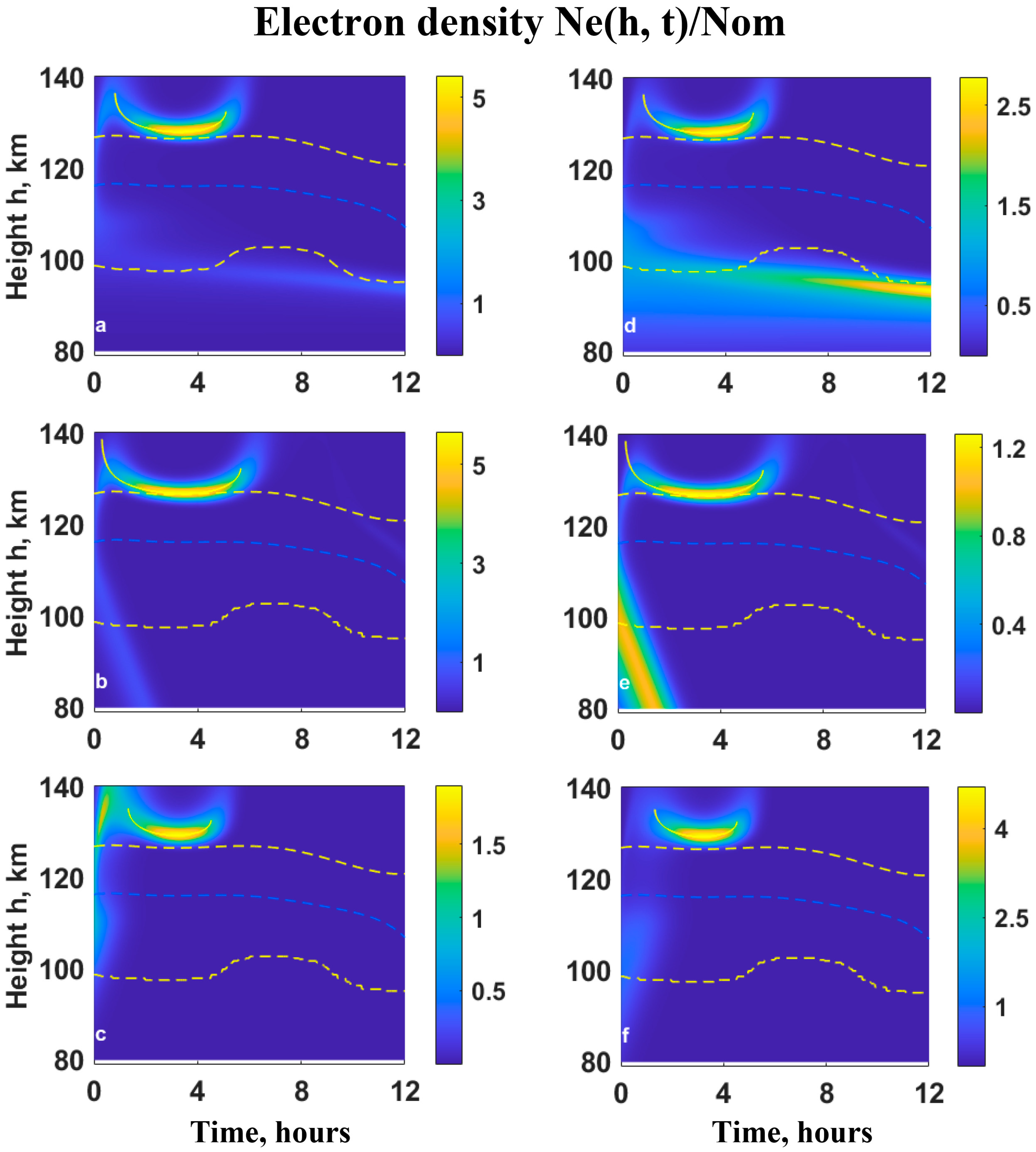
We will demonstrate the behavior of the ion/electron density height profile $N_e(z,t)/N_{om}$ and formation of the Es-type high-density thin layer (with peak density $N_{em}/N_{om}>1$), $H_{ic}(t=t_o)>H_{ic}(t>t_o)$ and/or ion/electron density depletion ($N_e/N_{om}<<1$). These phenomena can be predicted by analyses of ions drift velocity ${\mathrm{w}}_i(z,t)$ (Figure 4a–c) and its vertical changes $\frac{\partial {\mathrm{w}}_{i\mathrm{v}}}{\partial z}$ (Figure 4d–f), which are estimated using HWM14 data of meridional $V_x(z,t)$ and zonal wind velocities $V_y(z,t)$ (Figure 3a,b).

Neutral wind leads to the existence of the regions where the condition $\left(\frac{\partial {\mathrm{w}}_{i\mathrm{v}}}{\partial z}\right)\min <0$ i.e., $C_{t\max }^{\prime }>0$ is satisfied (Figure 3 and Figure 4). Figure 5 shows that close to the above-mentioned regions, the formation of the Es layers and their localization occur at regions with ${\mathrm{w}}_i=0$ (all panels) and ${\mathrm{w}}_{i\mathrm{v}}\to 0$ (Figure 5a,d). For the used horizontal wind profile (Figure 3) the high-density Es layer $N_{m1}/N_{om}=5.4$ (with $H_{ic}=1.8 \mathrm{km}$) is formed for a time around $t-t_o\le 3-5 \mathrm{h}$ (Figure 5a,d) at the location of the ion drift velocity node $h_{m1}=128 \mathrm{km}$ (${\mathrm{w}}_i=0$). Additionally, the secondary Es layer $N_{m2}/N_{om}=1.02$ is formed at a time $t-t_o=12 \mathrm{h}$ at lower heights ($h_{m2}<100 \mathrm{k}\mathrm{m}$) and it descends towards the height about $h_{m2}=93.4 \mathrm{km}$, where ${\mathrm{w}}_{i\mathrm{v}}\to 0$. When the density peak height of the ion/electron initial distribution is relatively higher $h_{om}=115 \mathrm{km}$ (close to the height region of the upper maximum of convergence rate $C_{t\max }^{\prime }>0$ and node ${\mathrm{w}}_i=0$), the density in the upper Es layer (with $H_{ic}=1.8 \mathrm{km}$) is higher $N_{m1}/N_{om}=5.4$ (Figure 5a) than when the initial distribution density peak height is lower $h_{om}=100 \mathrm{k}\mathrm{m}$, ($N_{m1}/N_{om}=2.8$, $H_{ic}=1.8 \mathrm{km}$) (Figure 5d). In these cases (Figure 5a,d), the lower location (close to the lower maximum of convergence rate $C_{t\max }^{\prime }>0$ around h = 99 km–104 km) of initial peak height (panel d, $h_{om}=100 \mathrm{km}$) causes higher density $N_{m2}/N_{om}=2.7$ in the lower Es layer ($h_{m2}=93.4 \mathrm{km}$) (Figure 5d) than in case of higher location $h_{om}=115 \mathrm{km}$ of initial peak height (Figure 5a).

Figure 5 also shows the existence of a divergence region $C_{t\min }^{\prime }<0$, where the ion/electron density continuously decreases/depletes ($N_e(z,t)/N_{om}<1$). The location of this region varies in the height interval from 116 km ($t=t_o$) to 112 km ($t-t_o= 12 \mathrm{h}$). For example, at the time $t-t_o=3 \mathrm{h}$, for the higher location of the initial peak height $N_e(h=116 \mathrm{km}, h_{om}=115 \mathrm{km}, t-t_o=3 \mathrm{h})/N_o(h=116 \mathrm{km}, t=t_o)\approx 0.02$ (Figure 5a), while for the lower location $N_e(h=100 \mathrm{km}, h_{om}=115 \mathrm{km}, t-t_o=3 \mathrm{h})/N_o(h=116 \mathrm{km}, t=t_o)\approx 0.09$ (Figure 5d).

Below the height regions of ions depletion (e.g., h < 110 km) where the ions drift velocity ${\mathrm{w}}_{i\mathrm{v}}\to 0$, at around h = 105 km the ion/electron total convergence rate is maximal $C_{t\max }^{\prime }\approx (2\pm 9)\times {10}^{-5} {\mathrm{s}}^{-1}$ and their ions converge into descending (${\mathrm{w}}_i\to -0$) Es-type layer ($N_e(z,t)/N_{om}>1$), with the continuous increase in densities and with the peak height located at about $h_{m2}=93.4 \mathrm{km}$ at $t-t_o=12 \mathrm{h}$. Here, the peak density of the formed Es $N_{m2}/N_{om}=1.02$ (Figure 5a) is smaller for the higher location of the ion/electron initial layer ($h_{mo}=115 \mathrm{km}$) compared to those for the lower location (close to the region with $C_{t\max }^{\prime }>0$) of the initial layer ($h_{mo}=100 \mathrm{km}$) when $N_{m2}/N_{om}=2.7$ (Figure 5d).

So, in the case of the presence of horizontal wind with only meridional and zonal components of velocities (Figure 3), two regions occur with condition $C_{t\max }^{\prime }>0$ (Figure 4). This leads to the formation of sporadic E with a double peak at about $h_{m1}=128 \mathrm{km}$ and $h_{m2}=93.4\mathrm{km}$ (Figure 5a,d). In this case, the upper Es layer is located at the height region with ${\mathrm{w}}_{i\mathrm{v}}=0$ ($h_{m1}=128 \mathrm{km}$) while the lower one descends to the height region where ions’ vertical drift velocity vanishes ${\mathrm{w}}_{i\mathrm{v}}\to 0$.

Figure 5b,e show that the downward direction of the vertical component of wind velocity $V_z<0$, which causes an increase in ion/electron downward flux, in case of $V_z=-4 \mathrm{m}/\mathrm{s}$, leads to the lower location $h_{m1}(V_z=-4 \mathrm{m}/\mathrm{s})=126.4 \mathrm{km}<h_{m1}(V_z=0)=128 \mathrm{km}$ of the ion vertical drift velocity node (${\mathrm{w}}_i=0$) and, therefore, the Es layer formation occurs at about $h_{m1}=126.8 \mathrm{km}$. Here, the higher location of the initial density peak height ($h_{mo}=115 \mathrm{km}$) and increase in ion/electron flux from upper regions to the region of ion drift velocity node h ≈ 126.4 km lead to the higher density $N_{m1}/N_{om}=5.6$ ($H_{ic}=1.7\mathrm{km}$) (Figure 5b) in the formed Es layer for a time around $t-t_o=3.4 \mathrm{h}$. Here, the relatively small value in the ion’s diffusive displacement to the heights above its convergence region also causes an increase in their peak density. In the case of the lower location, below the divergence region (about height 116 km) of the initial layer ($h_{mo}=100\mathrm{km}$), the increased downward flux of ions, caused by the downward vertical wind $V_z=-4 \mathrm{m}/\mathrm{s}$, leads to the formation of sporadic E with relatively lower density, $N_{m1}/N_{om}=1.3$ ($H_{ic}=1.7\mathrm{km}$) and at the lower location 126.4 km (Figure 5e), than in the case of higher location of initial density peak (Figure 5b).

Figure 5b,e show that the downward wind with additional depletion around the h ≈ 121 km region (Figure 2b,e) causes a relatively higher decrease in ion electron density, compared to the case of the wind with only horizontal components of velocity.

In the case of downward vertical wind velocity, secondary high-density Es layers are not formed at the lower heights of h < 110 km. This is because, unlike the case of wind with only horizontal velocity components, the region ${\mathrm{w}}_{i\mathrm{v}}\to 0$ does not occur and the ions/electrons layer descends with a velocity close to neutral vertical wind velocity ${\mathrm{w}}_{i\mathrm{v}}\approx -4 \mathrm{m}/\mathrm{s}$ (${\mathrm{w}}_{i\mathrm{v}}\approx V_z$) without significant changes in its density (Figure 5b,e). During the downward drift with velocity ${\mathrm{w}}_{i\mathrm{v}}\approx -4 \mathrm{m}/\mathrm{s}$, the ion/electrons cross the region of their convergence rate maximum (around h = 99–104 km) within a short time (about 1 h). For the values, $C_{t\max }^{\prime }\approx 2\cdot {10}^{-5}{\mathrm{s}}^{-1}$ this does not lead to a significant increase in the ions/electrons density, neither in the case of higher ($h_{mo}=115\mathrm{km}$) nor lower ($h_{mo}=100\mathrm{km}$) location of the initial layer. As a result, the formation of the secondary Es-type layer ($N_e(z,t)/N_{om}>1$) at lower heights <110 km does not occur. Figure 5c,f show that the wind velocity component directed upward $V_z>0$ causes the additional upward drift of ions/electrons, i.e., reduction of their downward drift velocity, as in Equation (7). In this case, the value $V_z=4 \mathrm{m}/\mathrm{s}$ leads to the relatively higher location of the ions drift velocity node ${\mathrm{w}}_i(h\approx 129.4\mathrm{km})=0$ (compared to $h_{m1}=128 \mathrm{km}$ in the case of $V_z=0$) and the Es layer formation occurs at about $h_{m1}=129.4 \mathrm{km}$. In this case of the higher location of the ion/electron initial layer ($h_{mo}=115\mathrm{km}$), the additional ion/electron upward drift and increase in ambipolar diffusion also lead to a lower density $N_{m1}/N_{om}=1.9$ (Figure 5c) in the formed Es layer than it was in cases of $V_z=0$ (Figure 5a) and $V_z=-4 \mathrm{m}/\mathrm{s}$ (Figure 5b).

The lower location of the initial peak height ($h_{mo}=100\mathrm{km}$) and upward vertical wind ($V_z=-4 \mathrm{m}/\mathrm{s}$) support the increase in ion/electron flux from lower to upper heights and their additional convergence at the height region of about 121 km (Figure 2f) leads to the relatively high density $N_{m1}/N_{om}=4.7$ in this Es layer formed at about 129.4 km height compared to the densities in Es layers formed for cases of $V_z=0$ ($N_{m1}/N_{om}=2.7$, $h_{m1}=128\mathrm{km}$—Figure 5d) and $V_z=-4 \mathrm{m}/\mathrm{s}$ ($N_{m1}/N_{om}=1.3$, $h_{m1}=126.8\mathrm{km}$—Figure 5e). In this case, in spite of the relatively lower value of the convergence rate, due to upward vertical wind ($\approx 4.9\times {10}^{-5}{\mathrm{s}}^{-1}$), the combined effect of horizontal wind direction, its shear and vertical wind gives high density ($N_{m1}(Vz=4 \mathrm{m}/\mathrm{s})/N_{1m}(V_z=0)\approx 1.7$) in the Es-type layer at about 129.4 km height.

The upward neutral wind and corresponding increased upward ion/electrons flux also result in their depletion in the divergence region (around 116 km). In both cases of the ion/electron initial layer being located at higher or lower altitudes, their depletion ($N_e(z=116 \mathrm{km}, t-t_o>0)/N_e(z=116 \mathrm{km},t=t_o)<1$) in the divergence region with $C_{t\min }^{\prime }<0$ for time of about $t-t_o>2.5 \mathrm{h}$ is bigger (Figure 5b,c,e,f), compared to the one during the absence of vertical wind (Figure 5a,d). However, for a time of about $t-t_o<2.5 \mathrm{h}$ the relatively small depletion at the height region around 116 km, due to ion/electron upward flux to this region by vertical wind velocity $V_z>0$, occurs at the lower location ($z_{om}=100 \mathrm{km}$) of the initial layer (Figure 5f).

Figure 5c,f also show that the increased ions/electrons upward flux at a lower height (h < 110 km) due to upward vertical wind $V_z>0$ also results in their density rarefication at lower height regions with maximal values of convergence rate (99–104 km) and the formation of the secondary Es-type layer at these height regions do not occur.

The upward/downward wind causes the vanishing of the region ${\mathrm{w}}_{i\mathrm{v}}\to 0$ at lower heights h < 110 km (${\mathrm{w}}_{i\mathrm{v}}\approx V_z$) and the formation of an Es-type layer in this region is less expectable. So, in this case of vertical wind velocity, the necessary condition $C_{t\max }^{\prime }>0$ for Es layer formation at regions about 99–104 km occurs, but it is not sufficient for its formation. It is important to note that the presence of condition $C_{t\max }^{\prime }>0$ for the formation of the Es-type is necessary but not sufficient. In the considered cases (Figure 5), the condition $C_{t\max }^{\prime }>0$ occurs for the whole night, but the development of the processes of ions/electrons convergence into a thin dense Es-type layer also depends on the initial distribution of these charged particles. For instance, if we use the same distribution for ion/electron density (Figure 2a,d) for different moments of the night, then the convergence of ions/electrons into the Es-type layer and its localization will occur at the regions where conditions $C_{t\max }^{\prime }>0$, ${\mathrm{w}}_{i\mathrm{v}}=0$ and ${\mathrm{w}}_{i\mathrm{v}}\to 0$ are satisfied at a particular moment of night mentioned above. This is not demonstrated for the sake of brevity.

Note that we have demonstrated theoretically the formation of the Es layer for one typical wind profile, including the HWM14 data, for the meridional and zonal wind velocities at mid-latitudes (45° N; 45° S). This methodology is not limited to HWM14 and can be applied to other model data, as well as measured wind profiles, including the data close to real time.

We can also apply our model to different initial distributions of charged particles, which fits both theory and measurements. In this case, by theoretically estimating the height profile of ions’ vertical drift velocity ${\mathrm{w}}_{i\mathrm{v}}$, as in Equation (7), and $\frac{\partial {\mathrm{w}}_{i\mathrm{v}}}{\partial z}$, the regions with conditions $\left(\frac{\partial {\mathrm{w}}_{i\mathrm{v}}}{\partial z}\right)\min <0$ ($C_{t\max }^{\prime }>0$) necessary for the development of ion/electron convergence into narrow dense Es-type layers also can be identified. This layer is located at the altitudes with minimal value of ions upstream and downstream flows (e.g., ${\mathrm{w}}_{i\mathrm{v}}=0$) or it moves to the region with ${\mathrm{w}}_{i\mathrm{v}}\to 0$ and $C_{t\max }^{\prime }>0$. In this case, the condition $C_{t\max }^{\prime }=(C_{\mathrm{v}}^{\prime }+C_{sh}^{\prime }+C_{\mathrm{v}z}^{\prime })\max >\frac{2D_a}{H_{ic}^2}$ necessary for sporadic E formation, for a particular mid-latitude region (with given B and I), is determined not only by the horizontal ‘windshear’ convergence rate $C_{sh}^{\prime }$, as in Equation (15), but also by the combined effect of rates caused by the realistic wind (three-dimensional) velocity magnitude, direction $C_{\mathrm{v}}^{\prime }$, as in Equation (14), and the vertical changes of vertical wind $C_{\mathrm{v}z}^{\prime }$, as in Equation (16). We note that in the lower thermosphere, the value of ions ambipolar diffusion, as in Equation (10), does not exceed 0.00001 m²/s. As a result, the condition $C_{t\max }^{\prime }>\frac{2D_a}{H_{ic}^2}$ at the initial time ($H_{ic}=10÷16\mathrm{km}$) is satisfied for the small values (e.g., $\pm 4 \mathrm{m}/\mathrm{s}$) of wind velocity. However, the effect of diffusion control on the Es layer is important during its formation (e.g., when $H_{ic}=1÷3\mathrm{km}$).

Below, we demonstrate the values of $C_{t\max }^{\prime }>0$ and $C_{t\min }^{\prime }<0$ (Figure 4 and Figure 5) and corresponding values of parameters $C_{\mathrm{v}}^{\prime }(z,t)$ and $C_{sh}^{\prime }(z,t)$. These values are determined by $\frac{\partial {\mathrm{w}}_{i\mathrm{v}}}{\partial z}$ profile, which in turn is estimated using the HWM14 data (Figure 3).

Figure 6 shows that the condition $C_{t\max }^{\prime }>0$ ($\left(\frac{\partial {\mathrm{w}}_{i\mathrm{v}}}{\partial z}\right)\min <0$) necessary for ion/electron convergence into Es-type thin layer (panels a and c) and the condition $C_{t\min }^{\prime }<0$ ($\left(\frac{\partial {\mathrm{w}}_{i\mathrm{v}}}{\partial z}\right)\max >0$) necessary for their divergence/depletion (panel b) are determined by the combined effect of convergence/divergence rates $C_{\mathrm{v}}^{\prime }(z,t)$, determined by wind velocity direction and magnitude, and $C_{sh}^{\prime }(z,t)$, determined by horizontal wind velocity vertical shear. For instance, in the case of only horizontal wind, the convergence rate in the upper Es layer, formed for time t − t_o = 3–5 h at heights about 126–130 km (Figure 5), $C_{t\max }^{\prime }\approx 0.0027 {\mathrm{s}}^{-1}$ (Figure 4 and Figure 5) is the sum of $C_{\mathrm{v}}^{\prime }\approx 0.00099 {\mathrm{s}}^{-1}$ and $C_{sh}^{\prime }\approx 0.0017 {\mathrm{s}}^{-1}$. The latter shows that in the upper Es layer (Figure 5) about 60% of ion/electron convergence into this layer is attributed to the ‘shear effect’ (by the presence of horizontal wind with vertical shear).

At lower heights (h < 110 km), the higher value $C_{t\max }^{\prime }\approx 9\cdot {10}^{-5} {\mathrm{s}}^{-1}$ in the Es layer (Figure 5a,d) is primarily caused by the convergence rate $C_{\mathrm{v}}^{\prime }$, which is determined by wind value and direction. In this region, the shear effect is negligible and even negative $C_{sh}^{\prime }<0$.

At the altitudes of approximately = 116 km, in the time interval t−t_o < 4 h, the magnitude of $C_{t\min }^{\prime }<0$ $\left(\frac{\partial {\mathrm{w}}_{i\mathrm{v}}}{\partial z}\right)\max >0$) reaches $\approx -0.002 1 {\mathrm{s}}^{-1}$, with approximately 30% ($C_{sh}^{\prime }\approx -0.0006 {\mathrm{s}}^{-1}$) of this value caused by the horizontal wind shear effect, while the remaining 70% ($C_{\mathrm{v}}^{\prime }\approx -0.0015 {\mathrm{s}}^{-1}$) is determined by the wind magnitude and direction.

At the heights of the peaks of the upper Es layer (h = 126 km–130 km), the divergence (≈116 km) and the lower Es layer (93–104 km), the component of the wind velocity has negligible contribution in the values of $C_{t\max }^{\prime }>0$ and $C_{t\min }^{\prime }<0$. However, the ions, due to their vertical drift caused by the vertical component of the wind velocity, pass through the region where only upward/downward vertical wind ($V_z=\pm 4 \mathrm{m}/\mathrm{s}$) causes the maximum convergence/divergence effect (height h ≈ 121 km); therefore, the vertical wind component influences the densities of ions in Es layers, as well as in the depletion regions.

The presented analytical and numerical study shows that the realistic (three-dimensional) profile of the neutral wind velocity in the lower thermosphere (h = 90 km–150 km) significantly determines the behavior of ion/electrons density in this region and therefore, the region of sporadic E (Es) formation and localization. Here, vertical profiles of the ions and vertical drift velocity and its vertical change, estimated by taking into account the vertical component of the wind velocity along with its horizontal component, influence the Es layer formation processes, since the above-mentioned profiles determine the condition, $\left(\frac{\partial {\mathrm{w}}_i}{\partial z}\right)\min <0$ (or $C_{t\max }^{\prime }>0$), necessary for ion/electron convergence into a narrow dense layer. Additionally, by the condition $\left(\frac{\partial {\mathrm{w}}_i}{\partial z}\right)\max >0$ (or $C_{t\min }^{\prime }<0$) the location of ion/electrons depletion regions is identified. It is important to take into account the presence of vertical wind because it affects both the location of regions of ions/electrons convergence into a narrow dense layer, as well as the dynamics of the development of these processes.

The presented theory can be extended by taking into account the production and loss rates (Q and L) of charged particles (e.g., NO⁺ and O₂⁺) in Equation (1), as well as considering the effects of the electric field and the ion drift caused by this field, in Equation (6). This extended study is planned for the near future.

The wind velocity profile given by the HWM14 is mainly determined by tidal motions and planetary waves [35]. The presented theoretical model allows its application for relatively short-term wind variations caused by AGWs and/or other dynamical processes. As a result, it is possible to study the regional features of the origin of the discussed ionospheric irregular structures caused by the above-mentioned processes. To study the feature of ions’ global and regional distributions, it is important to consider molecular ions (e.g., NO⁺ and O₂⁺), along with metal ions (e.g., Fe⁺, Be⁺) in the three-dimensional wind. This is also the subject of future studies.

4. Conclusions

(1) The behavior of the ion/electron concentration and the possibility of the formation of an Es-type layer, as well as their depletion processes under the influence of three-dimensional, which takes into account its vertical $V_z$ component along with the meridional $V_x$ and zonal $V_y$ components of the velocity $V$, are shown. In this case, the presence of a minimum negative value of the vertical change of the vertical drift velocity of ions $\left(\frac{\partial {\mathrm{w}}_{i\mathrm{v}}}{\partial z}\right)\min <0$ in the lower thermosphere, as the main condition for predicting the formation of the Es layer [26], was extended analytically and with appropriate numerical methods, in case of presence of the vertical component of the wind velocity $V_z$.

(2) Using the analytical approach for ion/electron concentration with consideration of ambipolar diffusion (17) shows that their narrow-layer total convergence rate $C_t^{\prime }=C_{\mathrm{v}}^{\prime }+C_{sh}^{\prime }+C_{\mathrm{v}z}^{\prime }$ ($\frac{\partial N_e}{\partial t}\propto -\frac{\partial {\mathrm{w}}_{i\mathrm{v}}}{\partial z}=C_t^{\prime }>0$) is determined by both horizontal and vertical wind velocity magnitude, direction ($C_{\mathrm{v}}^{\prime }$) and vertical change ($C_{sh}^{\prime }$ and $C_{\mathrm{v}z}^{\prime }$); see Equations (14)–(16). The vertical movement of the ion/electron layer and, accordingly, the localization of the Es-type layer in the regions of the minimal reduction (or with ${\mathrm{w}}_{i\mathrm{v}}=0$) of their lower and upper fluxes or regions where these fluxes vanish (${\mathrm{w}}_{i\mathrm{v}}\to 0$), is determined by the profile of the ions vertical drift velocity ${\mathrm{w}}_{i\mathrm{v}}$, as in Equation (7). In a given region (with particular B and I), it is possible to identify the regions of the development of ion convergence $C_{t\max }^{\prime }>\frac{2D_a}{H_{ic}^2}$ (Es-type layer formation) and their depletion conditions $C_{t\min }^{\prime }<0$. The convergence ($C_{\mathrm{v}z}^{\prime }>0$)/divergence ($C_{\mathrm{v}z}^{\prime }<0$) factor caused by the vertical wind is also influenced by the neutral particles’ wind velocity profile.

(3) Downward/upward vertical wind will shift the convergence regions (with ${\mathrm{w}}_{i\mathrm{v}}=0$ or ${\mathrm{w}}_{i\mathrm{v}}\to 0$) down/up, respectively, from their locations that existed in the case of just meridional and zonal winds. In the case of the presence of the wind velocity vertical component, the rates of convergence and divergence of the ions are different from their values in the case of just a horizontal wind.

Along with the profiles of the meridional ($-C_x$, $\partial C_x/\partial z$) and zonal ($-C_y$, $\partial C_y/\partial z$) factors of the wind velocity, the ones of the vertical wind factor ($C_z$) and its vertical change ($-\partial C_z/\partial z$) are important in the height profile of the ion drift velocity ${\mathrm{w}}_{i\mathrm{v}}$ and its vertical change $\frac{\partial {\mathrm{w}}_{i\mathrm{v}}}{\partial z}$ (see Figure 1). In this case, it is shown for the first time that the upward constant wind ($V_z>0$), like the northward wind ($V_x>0$), causes the convergence of ions with the maximum rate in the region of the maximum of $-\partial C_z/\partial z$ (h ≈ 121 km), where the collision frequency of ions-neutrals is equal to their cyclotron frequency ${\nu }_{in}={\omega }_i$ (Figure 1). In this height region, a downward wind ($V_z<0$), like a southward one ($V_x<0$), causes ion/electron depletion (Figure 2).

(4) The significant influence of horizontal wind, ions diffusion and their initial distribution, as well as the vertical wind on the behavior of ions/electrons and, therefore, the formation of Es-layer (as well as ion density depletion) has been demonstrated by numerical simulations (Figure 2 and Figure 5).

Accordingly, at first, the behavior of ions/electrons in the presence of only vertical wind was demonstrated (Figure 2), then the case of only horizontal wind determined by typical HWM14 data was considered (Figure 3) and, finally, the case of three-dimensional wind with the horizontal and vertical components was considered.

The vertically upward/downward component of the three-dimensional wind velocity will shift the regions of ion convergence (e.g., ${\mathrm{w}}_{i\mathrm{v}}=0$ or ${\mathrm{w}}_{i\mathrm{v}}\to 0$) upward or downward, respectively, and change both the location of the formed Es layer and its density relative to values of corresponding parameters estimated in the case of only horizontal wind (Figure 5). Here, the increase in diffusive displacement towards the upper regions (e.g., h > 120 km) also reduces the density of the upper Es-layer and increases it at the lower location.

The location of the initial ion/electron layer relative to the expected regions of convergence, as well as the ions drift caused by the vertical wind, influences the conditions for their convergence into a narrow layer in these regions (Figure 4 and Figure 5). For example, in the lower regions (h < 110 km), due to the downward/upward drift of ions (${\mathrm{w}}_{i\mathrm{v}}\approx V_z$), caused by downward/upward wind, respectively, the ions localization does not occur in the regions with ${\mathrm{w}}_{i\mathrm{v}}\to 0$ (Figure 5b,c,e,f), which appeared in cases of only horizontal wind (Figure 5a,d). So, the presence of a maximum rate of convergence ($C_{t\max }^{\prime }>0$) in the lower regions may not be sufficient for the formation of a high-density Es layer during the vertical wind.

In the case of three-dimensional wind with an upward component (Figure 5f), the formation of an Es layer with a density higher than in the case of only horizontal wind was shown (Figure 5d). In this case, the additional convergence caused by the vertically upward wind in the region increases the convergence caused by the horizontal wind in the regions close to the ion vertical drift velocity node.

(5) In the region of maximum ion/electron divergence $\left(\frac{\partial {\mathrm{w}}_i}{\partial z}\right)\max >0$ (or $C_{t\min }^{\prime }<0$) (e.g., at a height of about 116 km), during the presence of vertical upward/downward wind the depletion of ion/electron concentration is higher than in case of the horizontal wind alone (Figure 5).

(6) The convergence/divergence factors caused by the values of both the horizontal wind vertical shear ($C_{sh}^{\prime }$) and magnitude, and the direction of the wind velocity ($C_{\mathrm{v}z}^{\prime }$), which determine the maximum rates of convergence ($C_{t\max }^{\prime }>0$) and divergence ($C_{t\min }^{\prime }<0$), have been shown for the whole considered nighttime interval (Figure 6).

(7) The vertical wind velocity used in the numerical simulations is much smaller in the lower thermosphere than its observed [41] and model horizontal wind averages [35]. This can be caused by the tidal motions, as well as the propagation of AGWs. In the presented theoretical model, the three-dimensional profile of the wind velocity, which takes into account the vertical component along with its zonal and meridional ones, is important for the prediction of the regions of the ion convergence and formation of Es layers, and also the regions of ion depletion. Therefore, consideration of the significant effect of the wind shear [3,38,39], as well as the wind velocity magnitude and direction [12,26], including the vertical wind described above, is important to study the regional and global distributions of the metal ions [34,46,47,48,49,50] that make up the lower thermosphere.