Profiling of Aerosols and Clouds over High Altitude Urban Atmosphere in Eastern Himalaya: A Ground-Based Observation Using Raman LIDAR

Abstract

Profiles of aerosols and cloud layers have been investigated over a high-altitude urban atmosphere in the eastern Himalayas in India, for the first time, using a Raman LIDAR. The study was conducted post-monsoon season over Darjeeling (latitude 27°01${}^{\prime }$ N longitude 88°36${}^{\prime }$ E, 2200 masl), a tourist destination in north-eastern India. In addition to the aerosols and cloud characterization and atmospheric boundary layer detection, the profile of the water vapor mixing ratio has also been analyzed. Effects of atmospheric dynamics have been studied using the vertical profiles of the normalized standard deviation of RCS along with the water vapor mixing ratio. The aerosol optical characteristics below and above the Atmospheric Boundary Layer (ABL) region were studied separately, along with the interrelation of their optical and microphysical properties with synoptic meteorological parameters. The backscatter coefficient and the extinction coefficient were found in the range from $7.15\times {10}^{-10}$ m${}^{-1}$ sr${}^{-1}$ to $3.01\times {10}^{-5}$ m${}^{-1}$ sr${}^{-1}$ and from $1.02\times {10}^{-5}$ m${}^{-1}$ to $2.28\times {10}^{-3}$ m${}^{-1}$, respectively. The LIDAR ratio varies between 3.9 to 78.39 sr over all altitudes. The variation of the linear depolarization ratio from 0.19 to 0.32 indicates the dominance, of non-spherical particles. The periodicity observed in different parameters may be indicative of atmospheric wave phenomena. Cloud parameters, such as scattering coefficients, top and bottom height, and optical depth for different cloud phases, have been evaluated. A co-located Micro Rain Radar has been used with LIDAR for cloud life cycle study.

1. Introduction

The dynamical interactions of aerosols, clouds, and water vapor constitute an active field of research as they affect the radiation budget of the earth’s atmosphere and hence the climate through their participation in the energy transfer process [1]. LIDAR measurements can provide accurate, vertically resolved information, including multi-layer scenarios of clouds and aerosols.

Several LIDAR-based observations have been reported with the assumption of range-independent LIDAR ratio (LR) [2,3,4,5,6,7,8]. However, such an assumption is not consistent with the actual atmospheric aerosol distributions and hence may lead to loss of information [9]. In the case of Raman LIDAR, Raman channel return can be used, along with the elastic channel, to determine the extinction and backscatter coefficients separately, as reported by various authors [10,11,12,13,14]. A new method was proposed by [15] to retrieve the aerosol backscattering coefficient from Raman return by comparing with the molecule-dominated signal from reference altitude. The aerosol backscattering coefficient, along with Mie LIDAR range corrected signal (RCS) and optimized LR, was used to calculate the aerosol extinction coefficient [15].

In general, LIDAR systems are used to obtain both optical and microphysical parameters, which may be considered a two-step inversion process. In the first step, the measured backscattered power is used to estimate the optical parameters [16,17,18,19,20,21,22]. These parameters are then used in the second inversion to obtain the microphysical parameters, such as number size distribution, refractive index, etc. [23,24,25,26,27,28,29,30,31,32]. The aerosol extinction coefficient retrieval method from the Raman channel involves numerical differentiation of the Raman channel return RCS, which generates errors due to noise susceptibility of the RCS [10,33,34]. In order to avoid such errors, one may use the technique of signal smoothing [35]. The retrieval technique can be improved further using near-range reference height [36]. The proper reference height can be determined using signal-to-noise ratio and normalized standard deviation [37].

Several studies across the world are available in the literature on aerosols and cloud characterization using ground-based LIDAR observations [38,39,40,41,42,43]. The LR was used in the chemical characterization of dust aerosols [41,42,44]. The spectral depolarization ratio was shown to differentiate ice from pure dust and smoke [40]. It was also found to characterize atmospheric pollen and different dust sources using depolarization ratio of different wavelengths [45,46]. Elastic and Raman channels were used to characterize the microphysical properties of aerosols [38,47,48].

The water vapor mixing ratio (WVMR) measurement was reported at a high altitude station in Reunion Island and validated with satellite data [49]. In another study, automated algorithms were used to retrieve aerosol and humidity parameters along with temperature from Raman LIDAR and radiosonde measurement [50,51,52,53]. The large changes in temperature and water vapor were detected in the first-ever decade-long WVMR profiling performed in Switzerland, Payrene area [54], where the variation in precipitable water vapor was found to be strongly correlated with surface relative humidity.

Several detection techniques depending upon specific atmospheric scenarios have been applied to use LIDAR for boundary layer determination [55,56]. The mixed layer depth (MLD) determination using the Harr wavelet method is considered to be the most robust technique [57]. It was shown that the water vapor Raman LIDAR was capable of retrieving profiles of turbulent variables up to third order during the daytime [58]. The nocturnal boundary layer height determined by the elastic LIDAR was correlated to surface meteorological and aerosol parameters [59]. It was also shown that the residual layer and mechanically-driven surface aerosol layer might not be properly distinguished from the nocturnal boundary layer [55,60]. The elastic 532 nm channel requires the first lag time correction in order to obtain reliable turbulence information from the boundary layer [61], whereas the extended Kalman filter approach enables one to retrieve and track the boundary layer parameters based on simplified statistics of the boundary layer dynamics without the need for signal smoothing [62]. It was shown in [63] that the wavelet covariance method performed better during the daytime, whereas at night, the inflection point method was found to be more effective in detecting the nocturnal boundary layer as well as the residual layer height. Another new method, like the Gaussian mixture model, was used for the classification of the altitude sequence of the sample, made with backscatter coefficient and color ratio [64]. However, in the case of the multiple elevated aerosol layers scenario, cluster analysis with RCS and its variance was found to be more reliable compared to the Gaussian mixture model [65].

Recently, it has been hypothesized [66] that the trapping of aerosols may occur up to a particular inversion strength and depth only, whereas the inversion at the boundary layer top does not always cap the aerosol vertical distribution. In another study, the polarized LIDAR was used along with CALIPSO to study the mega dust storm in China, including its origin, transportation, and removal processes [67]. The microphysical and optical properties of the triple-layered vertical aerosol structure formed by the dust storm were studied in detail, and the bottom layer was found to be mixed with local anthropogenic aerosols. The elevated aerosol layers were probed by LIDAR along with satellite [68]. Several methods for aerosol and cloud detection, using different parameters, exist in the literature, such as the slope of logarithm of RCS along with the raw signal, backscattering coefficient of elastic channels, color ratio, and depolarization ratio [69,70,71,72].

The thermodynamic phase of clouds was studied extensively using linear depolarization ratio (LDR) and cloud top temperature (CTT) [43,73]. Ground-based LIDAR measurement was found to be more effective in discriminating ice and water clouds compared to satellite-based observation [74,75]. The presence of supercooled water was distinctly observed by [74]. It was possible to clearly differentiate between the stratocumulus and cirrus cloud [76] in a study in Durban, South Africa. Several in-depth studies of cirrus clouds characterization were conducted [39,77,78,79] using ground-based LIDAR observation. Aerosol-induced microphysical changes in the Altocumulus cloud were also studied in detail using Raman LIDAR and Doppler LIDAR [80].

In the Indian context, some important studies conducted in the recent past using ground-based LIDAR observations are worth mentioning. The air pollution ‘atlas’ over the Indian subcontinent was prepared using CALIOP data, a space-borne LIDAR to show the three-dimensional aerosol distributions over the subcontinent [81]. The vertical profile of aerosol extinction coefficient was found to gradually change from south to north of India from a broad layer structure to an exponentially decreasing extinction profile with increasing altitude. It was reported that within the altitude of 2000 m, the smoke dominated over northeastern parts of India while the polluted dust dominated all over the rest of the Indian subcontinent [81]. The effect of downwind transported agricultural crop residue burning and associated radiative forcing was also studied in Hyderabad, a metropolis in southern India [82]. The seasonal variation of aerosol and cloud properties was studied [83] and aerosol optical depth (AOD) was determined using elastic channels of LIDAR and compared to those obtained from AERONET and MODIS [84] over Manora peak, a high altitude station (1950 masl) in the western Himalayan region. The micropulse LIDAR observation of seasonal characteristics of aerosols were performed in tropical coastal regions in southern India as well [85].

The Raman LIDAR was used to study aerosol extinction and backscattering coefficient along with LR over the plain land regions, namely, Gwal Pahari, Pune, Gadanki, and Ahmedabad, as well as over the Indian Ocean [86,87,88,89,90,91]. The characteristics of cirrus clouds in Gwal Pahari and Gadanki were also studied by [92,93,94], respectively. The Raman LIDAR study in Palampur, a high-altitude station in the western Himalayas, using glued signal showed that, though the atmosphere above 4 km was quite free from aerosols, the cloud appeared at 7–8 km [95]. In another work in the Himalayan Tibetan Plateau (HTP) using Mie LIDAR and range independent 30 sr LR value, the contribution of aerosols was found to be mostly due to the transboundary transport of black carbon (BC) particles arising from the massive biomass burning in south Asia [96].

The high-altitude elevated aerosol layers absorb solar radiation and produce atmospheric dynamic feedback, which is known as the elevated heat pump mechanism. It enhances the snow melt in the Himalayas and Tibetan Plateau [97]. Moreover, optically thick clouds occurring below an aerosol layer enhance the absorption by aerosols above clouds [98]. In order to understand the role of aerosols in Himalayan climate change, a range-resolved aerosol and cloud characterization study is necessary. In addition to the several surface air quality and aerosol studies [1,99,100,101], investigations based on the remote sensing measurement of aerosol and cloud layer optical properties were also performed over the central and western Himalayan region in India [83,84,95,102,103,104,105,106,107,108,109]. On the other hand, despite several studies on surface air quality and aerosols over the eastern Himalayas [110,111,112,113,114,115,116,117], it has remained unexplored and virgin in terms of vertical profiling using ground-based LIDAR observations. The topography of the eastern Himalayas, with an abrupt rise from the Indo-Gangetic plain, is distinctly different from those of central and western Himalayas [118]. Moreover, the moist sub-temperate climate with heavy precipitation from June to September and moist, dense evergreen forest adds to the distinct features of the eastern Himalayas. It is imperative to have a good understanding of the vertical profiling of aerosols and clouds over this part of the Himalayas that is climatically vulnerable and ecologically fragile due to its proximity to glaciers and rich biodiversity.

In this region, amongst the dry season months, the most favorable months are found to be September and October in the post-monsoon season, when our study location, Darjeeling, experiences both the local and transported aerosols. Most importantly, the site experiences less occurrence of hill fog/near surface clouds, common enough phenomena here which would otherwise hinder our observation. The major objectives of the present study may be itemized as follows. (1) understanding of the range-resolved optical properties of aerosols and clouds; (2) boundary layer detection and range-dependent LR and (3) study of the development of cloud layer till the initiation of precipitation. To this end, we have studied the vertical profile of aerosol extinction and backscattering coefficients, WVMR, and LR using a Raman LIDAR. In order to understand the topographical effect on boundary layer dynamics, we have studied atmospheric boundary layer (ABL) height at day and night both. Cloud development has been studied using the colocated Raman LIDAR and micro rain RADAR. In addition, we have performed a periodicity analysis which may help us to understand the cause of certain phenomena as well as the interrelationship between different observables, if any.

2. Site Description and Synoptic Meteorology

The present work describes the study performed at Darjeeling (2200 masl), a popular tourist destination in Eastern Himalayas. Figure 1 shows the sampling location, Bose Institute campus (latitude 27°10${}^{\prime }$ N longitude 88°36${}^{\prime }$ E). A detailed description of the site is given in [110]. This region has a steep staircase topography, rising from the Siliguri at the foothills to Darjeeling within an aerial distance of 59 km. With the complex labyrinthian mountains with bold spurs, ridges, and valleys, it experiences greatly varying weather with heavy precipitation in monsoons.

The experiment was performed post-monsoon during September–October 2016. In this study period, the average temperature and relative humidity remained around $(13.08\pm 2.72)$ ℃, and $(82.1\pm 10.9)\%$, respectively. The average value of vertical wind speed was found to be around $(0.05\pm 0.04)$ m/s. The details of meteorological parameters of the post-monsoon season in Darjeeling have been reported earlier [113].

3. Instrumentation, Data, and Methodology

3.1. Instrumentation and Data

A manually controlled multiwavelength Raman LIDAR, developed by Raymetrics, was installed at the Bose Institute campus, Darjeeling, for vertical profiling of atmosphere [119,120]. The emitting system of this LIDAR consists of a frequency tripled ND: YAG laser emitting pulsed laser beam of 355 nm, 532 nm, and 1064 nm wavelength pointed vertically upward. The receiving system contains three elastic channels corresponding to 355 nm, 532 nm, and 1064 nm wavelength and two Raman channels of 387 nm and 408 nm wavelength. The Raman channels of 387 nm and 408 nm are the Stokes return of 355 nm incident wavelength for nitrogen and water vapor, respectively. It is designed based on the Cassegrain optical telescope, which has a receiver field of view of 1 milliradian with a vertical resolution of 7.5 m, the temporal resolution of the raw profile being 1 min. The returning signal is detected by photomultiplier tubes and converted into a resulting LIDAR signal by an A/D converter. It samples and digitizes the LIDAR signal with a 40 MHZ sampling rate, which corresponds to a 7.5 m vertical resolution. It is applicable for LIDAR signals coming from short distances within 8–10 km. The photon counting mode is used to detect low-intensity LIDAR signals above 8 km by photomultiplier tube with a 250 MHZ sampling rate. This sampling rate enables one to collect at least 1000 laser shots in order to lower the statistical fluctuation and obtain a satisfactory signal-to-noise ratio (SNR).

LIDAR signal processing includes the elimination of background atmospheric skylight and electronic noise due to instrumentation. The background is evaluated by selecting a range where the signal is quite stable, and the mean value at that range is minimum. The effective range of that signal is restricted up to that altitude. In order to generate a range-corrected signal (RCS), the range-related attenuation from the atmosphere was compensated by distance square law correction at each data point. A running low pass derivative digital filter with a variable path was applied to remove the high-frequency components, and the dataset was smoothed by least square fit with second order polynomial.

The LIDAR data were collected in the month of September and October 2016. We were able to collect nighttime data for seven days, three in September and four days in October, within this period. Daytime observation was performed on one day in October. In the case of nighttime measurement, the raw signal and RCS data of 7.5 m vertical resolution for elastic and Raman channels were collected. For daytime measurement, only the elastic channels were used as the Raman signal was too weak to be detected in the presence of strong daylight background. The cross and the co-polarized component of the 532 nm elastic channel were used for Linear depolarization ratio (LDR) estimation. The mathematical formalism for the retrieval of aerosol and cloud optical properties from the LIDAR signal are given in Appendix A.

A Micro rain Radar (MRR-2, METEK Technologies, Germany) was used here to detect the precipitation initiation time and its starting altitude. It is a vertically pointed Frequency Modulated Continuous Wave (FMCW) Radar, which transmits 24.1 GHz radiation at a bandwidth of 50 MHz vertically into the atmosphere. The radar reflectivity increases inside the cloud in the melting layer due to the difference in the refractive index of water droplets and ice aggregates in this frequency range [121]. The MRR, along with the LIDAR, was used for the case study of a cloud life cycle.

The specific humidity and temperature, along with zonal and meridionial wind velocity data from the European Center for medium-range weather forecast (ECMWF) re-analysis (or ERA) (https://cds.climate.copernicus.eu/cdsapp, accessed on 17 November 2022) were used for the calibration of the water vapor mixing ratio (WVMR) at different altitudes and the detection of cloud phase and periodicity analysis, respectively. HYSPLIT back trajectories of 120 h were used to compare the mixed layer depth from the present study and identify the source regions of the aerosol layers. The altitude was provided as an input of HYSPLIT by averaging the layer base and top.

3.2. Methodology

The raw data were stored at a 7.5 m altitude bin. However, for the present analysis, the effective spatial resolution of 120 m was determined by varying the number of points of sliding linear fit in order to resolve two narrow and well-separated structures in the aerosol extinction profile [122]. It also reduced signal fluctuations with minimum loss of information. In order to have credible results, the LIDAR measurement was obtained for the altitude range from the overlap height to the altitude where SNR remained above the threshold value. In some of the previous studies, the threshold was taken to be 10 [123,124,125]. In our case, up to 5 km in altitude, the SNR stayed above 1000 for aerosol/cloud layer-free days. In the presence of dense aerosol/ cloud layers, the SNR varied between 10 to 100 at the layer top region.

The aerosol extinction coefficient (${\alpha }_a$) and backscattering coefficient (${\beta }_a$) for every 30 min interval were evaluated using the retrieval technique mentioned in Appendix B (Equations (A7) and (A8)) using $RC{S}_{355}$ and $RC{S}_{387}$ for 120 m altitude resolution. The statistical fluctuations present in the signal could introduce large fluctuations in the derivative involved in Equation (A7). Three different methods, named ‘linear’, ‘quadratic’, and ‘averaged’, were used to identify the one with the least effect of fluctuation for further discussion.

In the first two methods, the term $ln\frac{N_m}{P_N{r}^2}$ in Equation (A7) was evaluated using $RC{S}_{387}$ with molecular density profile at an interval of 7.5 m. In the ‘linear’ method, this term was then fitted with a linear function in a 120 m bin, and the derivative was calculated from the fitted linear polynomial. In the case of the ‘quadratic’ method, a second-order polynomial function was used in a 120 m altitude bin to calculate the derivative. Finally, for the ‘averaged’ method, the RCS, as well as the molecular density, was averaged at 120 m intervals, and then the gradient of the term was calculated. The ${\alpha }_a$ values calculated in three methods were compared for different altitude ranges, and the ‘averaged’ method was found to have the fewest fluctuations. The ${\beta }_a$ was calculated using selected ${\alpha }_a$, and the corresponding LR was evaluated using their ratio. The reference altitude for the evaluation of ${\beta }_a$ was taken as the altitude for which ${\alpha }_a$/${\alpha }_m$ becomes negligible [126].

Here we would like to mention that ${\alpha }_a$ can be negative for certain cases Appendix B.1. In the present study, the ${\alpha }_a$ with negative values have been taken to be ${\alpha }_a=0$.

3.2.1. ${\alpha }_a$, ${\beta }_a$, LR, LDR and AE

The ${\alpha }_a$ and ${\beta }_a$ for each aerosol and cloud layer were calculated by the retrieval technique mentioned in Appendix B. The optical depth of the aerosol and cloud layer was evaluated by integrating ${\alpha }_a$ from the layer base to the layer top. All the aerosol layers corresponding to the same source were grouped together using the HYSPLIT back trajectory of 120 h. The aerosol layers from each source were categorized into two subgroups of coarse and fine mode dominating layer. For each subgroup, the ${\alpha }_a$, ${\beta }_a$, LR, LDR, and AE were calculated. The Angstrom exponent (AE) was calculated from the elastic backscattering coefficient of 1064 and 355 nm channels.

The depolarization channels have been calibrated using the $\pm 45$° calibration method [127]. The LDR was estimated using cross and co-polarized components of 532 nm channel using the expression LDR $=\left({\beta }_{532}^{\perp }\right)/\left({\beta }_{532}^{\Vert }\right)$, where ${\beta }^{\perp }$ and ${\beta }^{\Vert }$ are the aerosol backscattering coefficient of the cross and co-polarized channels corresponding to 532 nm. The thermodynamic phase of the cloud was detected by CTT, found from the reanalysis temperature data. The ${\alpha }_a$, ${\beta }_a$, LDR, LR, and cloud optical depth (COD) were studied and compared with the existing literature. Only one event for the cirrus cloud was observed in the study period.

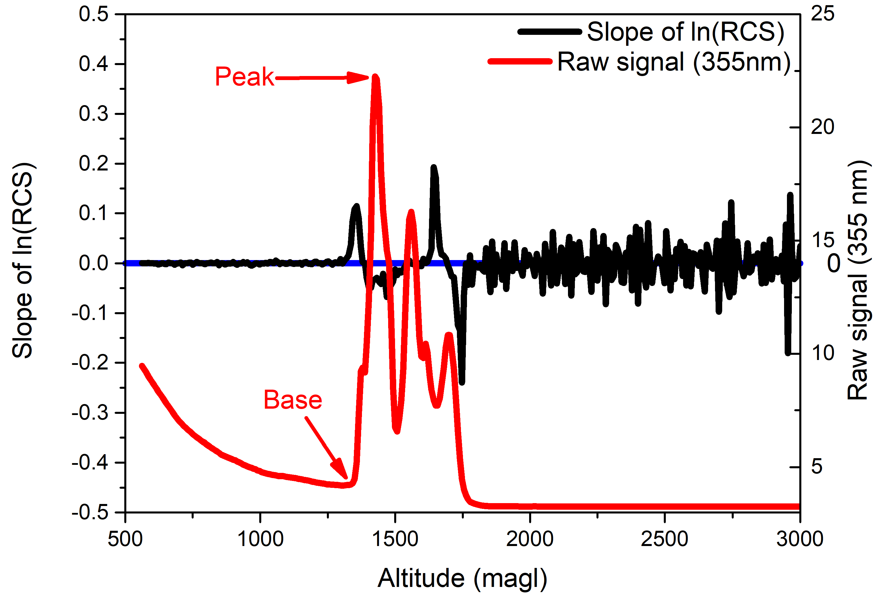
3.2.2. Aerosol and Cloud Layers

The aerosol or cloud layer base altitude can be defined as the altitude above which the density of aerosols increases abruptly, or the hydrometeors appear. This change in constituents would lead to a sharp increase in the backscatter signal indicating the location of the layer base. In the present study, in order to reduce the variability range of clear sky signal, the slope of $ln\left(RCS\right)$ with respect to altitude was used to detect the elevated aerosol layer boundary [128]. The altitude at which the signal started to increase (positive signal slope) corresponds to the layer base, whereas the slope of $ln\left(RCS\right)$ returned to the clear sky value at the layer top. The slope of $ln\left(RCS\right)$ and the raw signal for 355 nm are shown in Figure 2 to demonstrate the change of the slope and signal in the case of an existing layer.

The ratio (Rat) of the peak value of the raw signal to the signal at the base level was used to classify it as an aerosol or cloud layer. If Rat crossed the threshold ($Ra{t}_{threshold}$ = 4 below 5000 m and $Ra{t}_{threshold}$ = 1.5 above 5000 m), it was considered as a cloud otherwise, it was taken as an aerosol layer [72,128,129]. In the case of the low cloud below 800 m, the attenuation of the signal due to blocking by hydrometeors decreased the Rat value below $Ra{t}_{threshold}$. Then the minimum value of the slope within the layer ($D_s$) was used to identify the layer. If $D_s<-7$, it was considered to be a cloud layer. If $ln\left(RCS\right)$ within the layer was lower than three times its standard deviation, it was considered noise and rejected from the analysis [128].

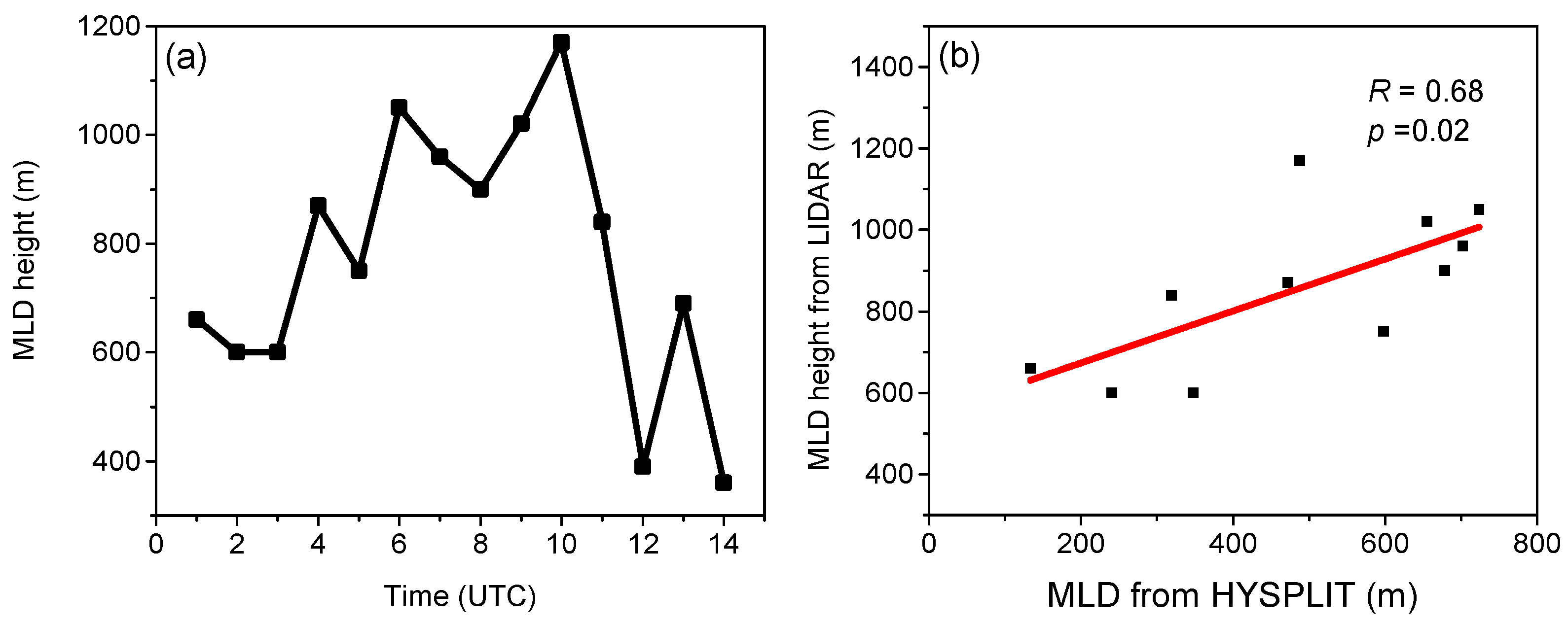
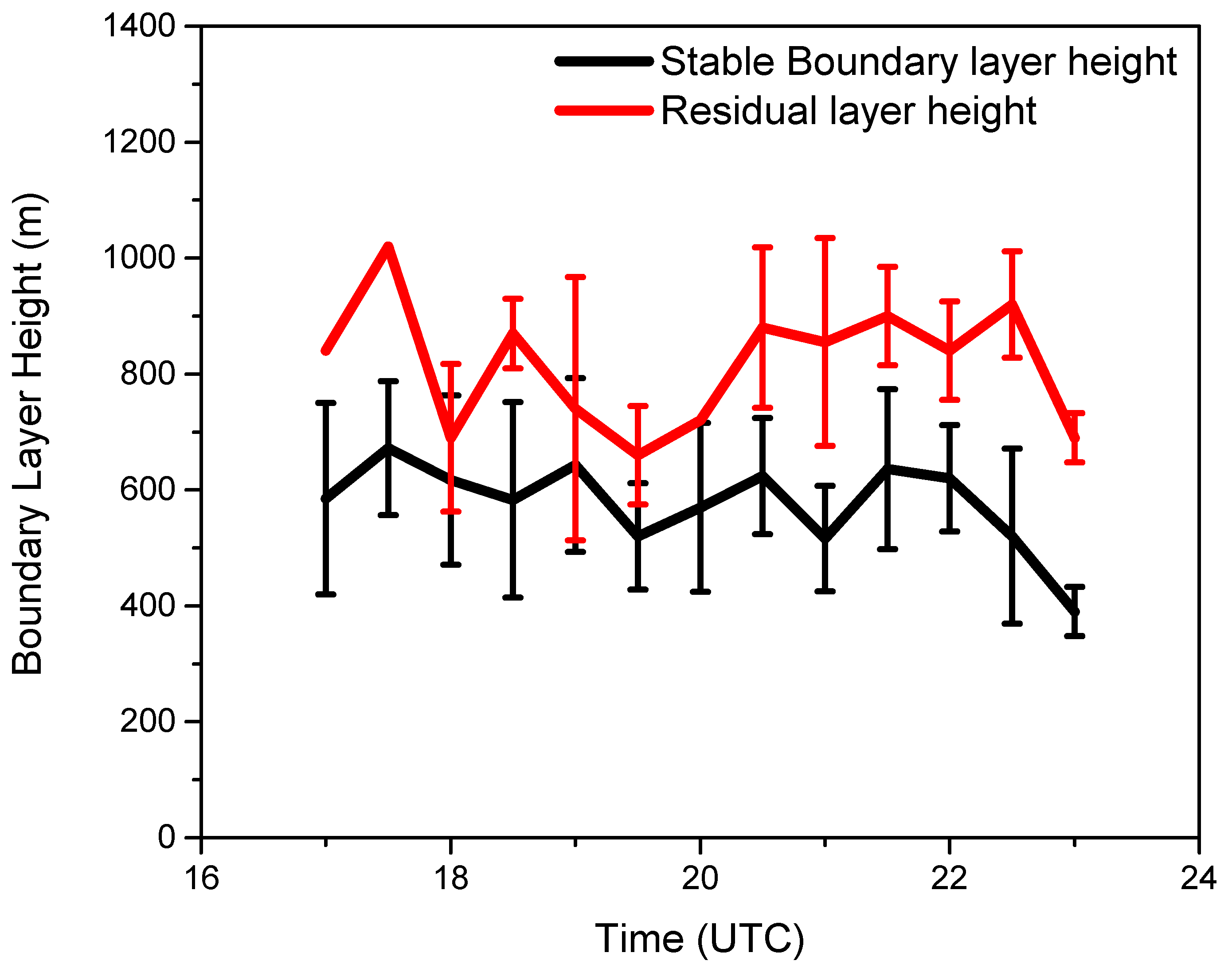
3.2.3. Atmospheric Boundary Layer

In the present study, Atmospheric Boundary Layer (ABL) was estimated using the non-hierarchical Cluster analysis (CA) method described in Appendix D. Here the optimal number of clusters was determined by both minimizing the Davies–Bouldin index Equation (A18), which measures the similarity between the clusters, and maximizing the Dunn index indicating compact and well-separated clusters Equation (A19). The mean $RC{S}_{355}$ and its variance at 30 min intervals were used here. The data were normalized by dividing all the values of each parameter by their maximum. The ABL top was estimated by the height at which the cluster change occurred [65] due to the sudden decrease of aerosol concentration at the ABL top, which maximizes the variance as well.

The vertical extent of convective mixing is termed as ‘mixed layer depth’ (MLD) [130]. The decaying convective mixing in the evening forms a neutrally stratified residual layer. At night the land surface cools faster than the earth’s atmosphere by emitting long wave radiation, which causes surface-based temperature inversion and hence stable boundary layer (SBL) formation [130].

In the present case, complete information could not be retrieved, at lower altitudes, due to the partial overlap of the laser beam and telescope field of view. The MLD was determined by applying the cluster analysis on the daytime data of LIDAR RCS and its variance from 60 m to 2000 m. The MLD was identified as the altitude above the overlap height (360 m), at which the first cluster change occurred.

For the SBL height determination, the nighttime LIDAR RCS and its variance within the altitudes 60 m to 1200 m were considered. There were multiple cluster changes in one profile, indicating multiple aerosol layers at night. The first one above 360 m was the SBL top, and the layers above it up to 1000 m were identified as residual layers [65]. The depth of the residual layer is usually identified as the space between the top of the SBL and the base of capping inversion [131].

A sample plot of mean and variation of RCS along with the stable boundary layer (SBL) and multiple residual layers are shown in Figure 3.

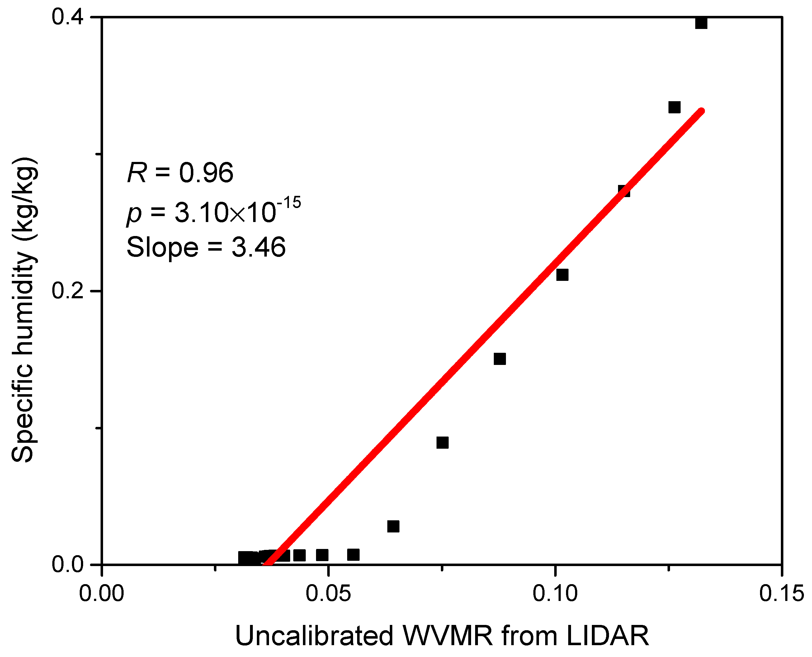
3.2.4. Water Vapor Mixing Ratio (WVMR)

The WVMR was retrieved using the standard method (Appendix C) [132,133,134]. It was calculated using 408 nm and 387 nm channel returns (Equations (A13) and (A15)). A low pass filter was applied in order to remove the unrealistic high values that appeared due to the noise fluctuation of RCS. If the raw signal of the 408 nm channel was reduced to less than 0.01 mv after a certain altitude, the WVMR above that altitude was taken to be zero. A careful analysis was needed here as it was observed that a similar reduction could also occur due to the cloud-induced extinction of the return signal of the 408 nm channel.

WVMR was calibrated using ERA-interim specific humidity profile in kg/kg dry air unit along with AWS situated at the station by linear fitting. The specific humidity reanalysis data and un-calibrated WVMR were averaged over the study period and fitted with a first-order polynomial. The slope of the fitting (Figure 4) was taken as the calibration constant.

Since the calibration constant varies with altitude due to different vertical processes of moisture transportation, the information of the specific humidity for the entire altitude range, including the low values at higher altitudes, was used for the calibration [135,136,137,138,139].

3.2.5. Atmospheric Dynamics and Periodicity

The normalized standard deviation (NSD), which is defined as the standard deviation of RCS normalized by its mean value for each point of range profile, may be considered as a measure of optical turbulence intensity [140,141,142]. We have studied the NSD profile of 355 nm for this analysis. The two 30 min intervals were selected in order to distinguish the NSD characteristics in the case of stratified and turbulent atmospheres.

The Lomb–Scargle periodogram (LSP) was used to study the frequency spectrum for the hourly data for every 120 m altitude ranging from 600 m to 4920 m. Details of the formalism were discussed in [116].

4. Results and Discussions

In the present section, we have described the LIDAR-derived quantities and their implications. The variations of the stable boundary layer (SBL) and residual layer, along with mixed Layer depth (MLD) over time, have been described. The vertical profiles of optical parameters and their variation, along with the water vapor mixing ratio (WVMR) in the absence or presence of cloud/aerosol layers, have been discussed within and above the Atmospheric Boundary Layer (ABL) separately. Depending on the source region, we have analyzed the aerosol layers at different altitudes. The cloud properties have been extracted to analyze the observed cloud layer characteristics. The formation and development of a cloud layer have been discussed using co-located LIDAR and MRR. The periodicity analysis of range corrected signal (RCS) and derived quantities are presented at the end.

4.1. RCS, ${\alpha }_a$, ${\beta }_a$, and LR

The variation of RCS${}_{355}$, RCS${}_{387}$, and derived aerosol parameters are shown in Figure 5 with three rows corresponding to the three different days. The mean deviation of aerosol extinction coefficient (${\alpha }_a$) evaluated using linear and quadratic fit compared to the ‘averaged’ method are of the order of ${10}^{-5}$ or higher. Moreover, the ‘averaged’ method gives the smoother variation of ${\alpha }_a$ compared to the other two methods and is used for the rest of the analysis.

In the first row, both the RCS show a monotonic behavior indicating the absence of aerosol and/or cloud layer. The backscattering coefficient (${\beta }_a$) was found to decrease sharply with increasing altitude. There were two increments of ${\beta }_a$ at 1000 m and 2000 m. The LIDAR ratio (LR) at 1000 m and 2000 m was found to be $59.06\pm 32.5$ sr and $32.61\pm 15.22$ sr, respectively. The decrease in ${\beta }_a$ resulted in the increase in LR at altitudes above 3000 m.

The second row (Figure 5) shows the presence of three elevated aerosol layers at altitudes 2000 m, 3000 m, and 4000 m. The corresponding RCS${}_{355}$ shows a peak, and RCS${}_{387}$, the Raman line from $N_2$, shows step-like behavior signaling a sudden change in $N_2$ concentration. They were identified as aerosol layers following the argument as discussed in Section 3.2.

The LR is evaluated from the ratio of the extinction to the backscatter coefficient. In the case of aerosol layers around 2000 m, LR is found to vary from $36.36$ to $130.3$ sr with an average of $70.58\pm 26.62$ sr. This value is comparable to results found by some other authors as well [143,144,145]. The LR for aerosols depends on its sources along with its aging and mixing processes over the transported path [145].

On the other hand, the larger variation of the values of LR inside the aerosol layers, above 2000 m, resulted in unusually large mean values as well as standard deviation. The larger drop in signal-to-noise ratio (SNR) and fluctuations in RCS induces larger variation in the LR values within the layer. Here, as seen in (Figure 5) LR varies between $30.38$ to $491.4$ sr, resulting in an average value of $160.85\pm 178.3$ sr.

The RCS${}_{355}$ peak and RCS${}_{387}$ step-like structure can be seen in the third row as well. This was identified as a cloud layer Section 3.2. In the case of clouds, the within-layer variation of LR is found to be much larger. The LR value for the cloud layer was found to vary between $60.2$ to $886.5$ sr with an average of $211\pm 269$ sr. Here there is an increase in ${\alpha }_a$ along with a large drop in ${\beta }_a$. In this case, the absorption of the LIDAR signal inside the cloud layer along with the multiple scattering might be responsible for the increase in the ${\alpha }_a$ value and hence the LR [146]. More investigation is needed to understand the large variation of both aerosol and cloud layers.

The ${\alpha }_a$ values in the first row were much lower than the days with aerosol and cloud layers. The aerosol diffusion, its vertical movement, and hence the stability is controlled by the strength of the temperature inversion layer [147,148]. The lower values of ${\alpha }_a$ may be due to the weaker inversion, which inhibited the formation of the aerosol layer and resulted in the comparatively low density of aerosols.

4.2. Atmospheric Boundary Layer

The complete cycle of evolution of MLD from 0000 UT to 1400 UT on 28 October 2016 is shown in Figure 6. The entire interval was controlled by solar convective activity, the local sunrise and sunset time being 0000 UT and 1130 UT, respectively. No cloud layer was detected by LIDAR on that day. MLD increased from 0300 UT to its maximum of 1200 m at 1000 UT despite its fluctuation around 0500 UT and 0800 UT. The time lapse between sunrise and the onset of MLD growth may be due to the sensible heat flux along with wind flow strength dependence of below-SBL region warming by shear-driven turbulence and resulting entrainment [149]. The fluctuations around 0500 UT and 0800 UT might be due to updraft and downdraft of the turbulent eddies resulting from intense convective mixing [57,150]. With the approaching sunset, MLD started to decrease after 1000 UT onwards. Thermal formation eventually ceases due to the decaying turbulence initiating the collapse of the mixed layer. In this situation, the aerosol accumulation in lower levels would be enhanced, leading to the increase in backscattering [151]. MLD in the present study is found to be positively correlated with HYSPLIT-generated MLD (Figure 6). In the present study, the residual layer was identified from the cluster analysis as the layer just above the SBL. Multiple layers were observed as shown in (Figure 3). The position of the residual layers varied from 720 m to 1020 m, with the most frequent position being at 840 m (Figure 7). In some cases, the error bars can be seen to be missing as the residual layer was not always visible. In the mountainous topography, the complex temperature inversion characteristics with multilayer structure were observed earlier [152]; the residual layer was shown to have two parts, the upper part being inconspicuous.

The interaction of the residual layer and SBL may occur via large-scale processes such as subsidence, mountain valley circulation, and gravity waves. These interactions lead to the formation of complex multilayer structures in temperature inversion and aerosol concentration in the mountainous urbanized region [152]. In the present study, the reasons for variations in the SBL and ABL top, as seen in Figure 7, might be due to unstable conditions along with interlayer mixing due to complex dynamics of terrain and the corresponding wind pattern. The presence of low cloud, a frequent occurrence at the present site, may induce error in the extraction of boundary layer heights [153,154,155].

The average height of SBL, in the present study, is found to be around $576\pm 75$ m. The temporal variation of average SBL height for the study period is shown in Figure 7. Its formation after sunset depends on surface radiative cooling as well as local topographical features. As mentioned earlier, the experimental site is located in a mountainous region with a staircase-like topology. The urbanized hill station with local anthropogenic activity has the potential to behave like the urban heat island. A similar study of the boundary layer formation process for an urban heat island in a mountainous region was conducted in detail in Sofia, Bulgaria [156].

4.3. Comparison of Vertical Profiles of Aerosol Optical Parameters between the Days with and without Aerosol and/or Cloud Layers

The entire study period was divided into two groups based on the absence (group 1) or presence (group 2) of aerosol layers and/or cloud layers. Group 1 consists of days having no aerosol or cloud layers. Days with at least one aerosol or cloud layer within 5000 m constitute group 2. The valid range of LR was reported to be within 0 to 200 sr for the aerosols trapped inside in planetary boundary layer [157]. The lowest LR for low light absorbing larger maritime aerosols was found to be around 20–30 sr, and the largest range for smaller highly absorbing urban haze was around 70–100 sr [158]. On the other hand, for heavily polluted cases, the LR was found to be greater than 100 sr in different studies [145,159]. So, while averaging, we set the upper boundary of the filter for LR to 200 sr. The quantitative analysis of the LR profile was performed up to 2000 m as at higher altitudes, the large variation in LIDAR SNR might introduce larger errors in the LR profiles [35].

The entire altitude range in the present study was divided into two regions separated by the top of the residual layer. The temperature inversion above the residual layer acts as a capping inversion at nighttime and stops the aerosol mixing. So, the region between the overlap region (360 m) and the average residual layer top height (960 m) is dominated by locally generated aerosols. The atmospheric phenomena in this region is discussed below Section 4.3.1. On the other hand, the altitude range from the residual layer top height to 5000 m is dominated by long-range transported aerosols. The observations in this altitude range are discussed below in Section 4.3.2.

4.3.1. Profiles within the ABL

The vertical profile of ${\beta }_a$, ${\alpha }_a$, LR, Angstrom exponent ($AE$), linear depolarization ratio (LDR) along with WVMR, for both group 1 and group 2 are shown in Figure 8, from 360 m to 960 m. The nocturnal SBL, around 588 m, shielded the aerosols transport at night. However, owing to aerosol penetration in the mixed layer throughout the day and its persistence in the residual layer at night, the aerosol concentration in this region remained higher than at other altitudes. It is dominated by locally generated aerosols from vehicular exhaust and biomass burning mainly.

Group 1

Figure 8 shows that ${\alpha }_a$ remains zero till 500 m and increases with altitude. ${\beta }_a$ is found to decrease till around 500 m, and then the rate of decrease with altitude becomes slower. LR remains zero till 500 m and then starts increasing with altitude. Beyond 700 m, LR increases sharply with altitude. AE increases till about 600 m and then remains almost constant with height. LDR decreases monotonically with altitude though the rate is slower beyond 800 m. WVMR also decreases slowly with altitude.

Group 2

A cloud layer was observed with its base around 600 m and top around 830 m. Figure 8 shows that both ${\alpha }_a$ and ${\beta }_a$ initially increase with altitude. ${\alpha }_a$ starts decreasing beyond 700 m, while ${\beta }_a$ starts decreasing at 600 m. LR increases initially and then changes its slope sharply around 700 m. LDR, as the figure shows, decreases monotonically till around 600 m. The rate of decrease becomes slower above this altitude. WVMR also decreases with altitude.

The difference between group 1 and group 2 bears the signature of higher loading of aerosols and water vapor along with the cloud layer observed around 600–830 m for group 2. The higher aerosol loading along with WVMR abundance (Figure 8) presented a favorable condition for cloud formation. The increase in ${\alpha }_a$ up to a higher altitude than ${\beta }_a$ may be due to small aerosol particles production near cloud vicinity [160] and multiple scattering inside the cloud by hydrometeors [161].

The AE values shown in the Figure 8 indicate the coarse mode aerosol dominance within ABL for both groups. The LDR values were similar for two groups up to 800 m. Above 800 m, the LDR for group 1 is indicative of higher nonsphericity of aerosols compared to group 2, as the higher WVMR for group 2 induces more sphericity.

The correlations between the different quantities within the ABL are given in the first two columns of

Table 1. The correlation coefficient (R) for linear correlation among LR, LDR and WVMR are shown in the table. All correlations are statistically significant with probability <0.05.

Correlation	Below ABL		Above ABL
	Group 1	Group 2	Group 1	Group 2
LDR-WVMR	0.47	0.95	0.94	−0.69
LR-LDR	−0.52	−0.93	0.48	0.45
LR-WVMR	−0.94	−0.78	0.45	−0.53

. LDR-WVMR correlation is positive for both groups. The decrease of WVMR with altitude may be due to the droplet formation by condensation on aerosols. This would create more spherical particles and cause a decrease in LDR. The droplet formation might also lead to an increase in ${\alpha }_a$ caused by the multiple scattering. It would increase LR resulting in a negative correlation between LR-LDR and LR-WVMR.

4.3.2. Profiles above the ABL

The vertical profile of ${\alpha }_a$, ${\beta }_a$, LR, AE, LDR, and WVMR for group 1 and group 2 are presented in Figure 9 from the altitude 1000 m to 5000 m. As the temperature inversion above the ABL caps the local aerosols within ABL, they are inhibited from entraining in the free troposphere region. So this region is dominated by long-range transported aerosols.

Group 1

HYSPLIT back trajectory for group 1 showed that the long-range transportation was predominantly from the Nepal region, which is rich in anthropogenic aerosols [114]. The anthropogenic plumes generated by biomass burning or vehicular exhaust contain black carbon (BC) as one of the significant components [162,163]. Both ${\alpha }_a$ and ${\beta }_a$ are found to decrease with altitude, the rate of change of the latter being more. This leads to an increase in LR up to 1400 m. Interference of scattered radiation from coarse mode scatterers may be responsible for the faster decrease in ${\beta }_a$. Above this, the rate of decrease of ${\alpha }_a$ may be more due to fewer aerosols as well as cloud condensation nuclei (CCN) due to a decrease in WVMR. Further increase in LR beyond 1800 m may be the result of low SNR [35]. AE value is less than 1 (Figure 9) up to 4000 m, indicating the presence of coarse mode aerosols. AE increases with altitude and becomes more than 2 beyond 4000 m, indicating the presence of very small particles. LDR decreases with altitude till 3000 m indicating more abundance of regular shaped aerosols with increasing altitude [145]. Above 3000 m, small aerosol abundance may result in a constant LDR. The LDR value above 3000 m is unusually higher compared to other studies [40,145,164,165] and needs further investigation. WVMR also decreases with altitude and becomes almost zero around 3000 m.

Group 2

The long-range transportation for group 2 was from the Bay of Bengal (BoB), passing over Bangladesh, NE India, and Bihar, which are neighboring states of West Bengal. So the aerosol types were mainly maritime and anthropogenic aerosols from vehicular exhaust [114]. The ${\alpha }_a$ and ${\beta }_a$, shown in Figure 9, are much higher compared to group 1 below 4000 m and 3500 m, respectively, due to the presence of cloud and aerosol layers. Since ${\alpha }_a$ depends on the rate of change of LIDAR return (Equation (A7)), the layers’ structures are more prominent in its variation. The presence of cloud around 1680 m resulted in the increase and then decrease in ${\alpha }_a$ as the beam encountered the cloud hydrometeors. The layered structure of ${\alpha }_a$ in the range 2000–4000 m reflects the presence of several aerosol layers. The sharp variation in ${\beta }_a$ in the altitude range 1000–2000 m may be due to the cloud hydrometeors.

${\beta }_a$ depends on the number density of aerosols and their back-scattering cross sections, later being dependent on their size and shape [Appendix A]. The marine aerosols have mainly the coarse mode particles of diameter >1 $\mathsf{\mu }$m [166], whereas anthropogenic plume aerosols have diameter ≤1 $\mathsf{\mu }$m [167]. The evaluation of x for these aerosols with incident 355 nm wavelength suggested a dominant contribution of Mie scattering for both types of aerosols as discussed in Appendix A. The greater abundance of WVMR for group 2 resulted in a higher CCN activation probability for the aerosols. This would increase their sphericity resulting in an increase in ${\beta }_a$ [168]. LR is found to increase up to 1500 m and then decrease. Further increase in LR, around 2000 m may be the result of low SNR [35]. AE variation is indicative of the mostly coarse mode dominance except in the aerosol layers around 3000 m and 3500 m. LDR variation indicates the variation in the sphericity of the constituents due to the presence of a cloud layer near around 1000–2000 m and the aerosol layers above. The air parcel ascent governs the initial decrease in WVMR. Its further variation may be controlled by the variation of the amount transformed to liquid water, which depends on the availability of condensation nuclei and surrounding meteorological conditions. The sharp decrease in WVMR with an altitude above 3500 m is due to low SNR of 408 nm raw signal.

Using Mie scattering for spherical particles, the single scattering albedo (SSA) calculation of core-shell combination among BC, sea salt, and sulfate were studied earlier [169]. It was shown that the BC shell-sea salt core combination has lower SSA than the BC core-sulfate shell combination, and all these combinations have enhanced absorption coefficients compared to the externally mixed case. The presence of a thin layer of cloud increases the probability of the mixing of BC with sea salt aerosols through core-shell combination. This enhancement in absorption resulted in an increase in the extinction coefficient and hence aerosol optical depth (AOD). In the case of group 2, the anthropogenic plume mixed with sea salt aerosols could lead to the core-shell combination and enhanced ${\alpha }_a$ due to an increase in absorption.

Let us now compare the observations for both groups. An increase in ${\alpha }_a$ near the vicinity of the cloud layer may be due to new small particle production and aerosol swelling as relative humidity increases near the cloud [160]. This may be the reason for the higher average standard deviation for ${\alpha }_a$ in the case of group 2 ($1.04\times {10}^{-3}$) compared to group 1 ($2.7\times {10}^{-5}$). The average standard deviations of ${\beta }_a$ are $3.28\times {10}^{-7}$ and $8.97\times {10}^{-6}$ for groups 1 and 2, respectively. It was higher for group 2 due to larger backscattering from aerosol and cloud layers. Above 4000 m, ${\alpha }_a$ and ${\beta }_a$ are almost the same for both groups due to the negligible amount of aerosols present. The low aerosol concentration and homogeneous vertical distribution above 3000 m were also reported in the literature [145].

LR was found to be higher for group 1, despite the presence of aerosols and cloud layers in group 2. This may be due to a larger increase in ${\alpha }_a$ compared to ${\beta }_a$ on 28 October 2016 caused by the increase in aerosol number concentration at that altitude. The corresponding increase in LDR indicates an increase in nonspherical aerosol concentration.

The celebration of Diwali (30 October 2016) with fireworks in India usually starts a few days earlier. The generation of huge amounts of aerosols due to fireworks was reported earlier [170]. In order to illustrate our argument, the increase in CCN concentration on Diwali day compared to non-Diwali day due to fireworks at night is shown in Figure 10. The generated aerosols and water vapor could be uplifted due to instabilities. This would induce a larger increase in ${\alpha }_a$ compared to that in ${\beta }_a$ and hence in LR.

The correlation between the different quantities is given in the last two columns of Table 1. ${\beta }_a$ and ${\alpha }_a$ for group 1 were found to decrease monotonically with altitude, indicating a sharp decrease in aerosol concentration with altitude. The less advection of aerosols along with water vapor decreased the ${\beta }_a$ and WVMR with altitude. The LDR also showed sharp a decrease with altitude. The regularly shaped non-absorbing particles at high altitudes might be the reason for LR decreasing with height as found by [145,171]. So LDR, LR, as well as WVMR is found to exhibit a positive correlation with each other.

The multiple aerosol/cloud layers were the result of the temperature inversions present in the atmosphere for group 2. This induces nonmonotonic behavior in WVMR, AE as well as LDR. The WVMR decreased with altitude, as it was advected from the ground by ascending air parcels and also got condensed to liquid water on the aerosols. The existence of clouds at different altitude levels induced multiple scattering by cloud hydrometeors, thereby increasing the ${\beta }_{\perp }$ component and hence LDR [146]. So LDR-WVMR became negatively correlated while LR-LDR is positively correlated as the multiple scattering by cloud hydrometeors increased ${\alpha }_a$ and hence increased LR in turn. This resulted in a negative correlation between LR and WVMR.

4.4. Characterization of Aerosol Layers

HYSPLIT back trajectories of 120 h were used to identify the source of the aerosol layers. The altitude was provided as an input of HYSPLIT by averaging the layer base and top. In

Table 2. Characteristics of the aerosol layers during the entire study period. The $LR>200$ sr and $LDR>1$ are exempted from this study. The reasons are explained in the text.

Source	Mode	Layer Base (m)	Layer Top (m)	Layer Thickness	${\mathit{\beta }}_{\mathit{a}}\times {10}^{-6}$ (m${}^{-1}$sr${}^{-1}$)	${\mathit{\alpha }}_{\mathit{a}}\times {10}^{-4}$ m${}^{-1}$	LR (sr)	LDR	AOD
BoB-Bangladesh-WB	Coarse	1550.3	1872.6	322.3	$3.8\pm 0.9$	$6.7\pm 3.8$	$127.0\pm 77.8$	$0.17\pm 0.01$	$0.27\pm 0.09$
BoB-Bangladesh-WB	Fine	2304.8	2564.7	260.0	$1.8\pm 0.5$	$27.6\pm 22.3$	$99.2\pm 57.3$	$0.24\pm 0.01$	$0.93\pm 0.76$
NE India	Coarse	2371.7	2512.7	141	$2.6\pm 1.9$	$7.6\pm 5.3$	$97.0$	$0.35\pm 0.07$	$0.25\pm 0.22$
NE India	Fine	2560.7	2831.3	270.5	$1.9\pm 0.6$	$29.9\pm 10.4$	$81.9$	$0.47\pm 0.05$	$1.13\pm 0.34$
Bangladesh- NE India	Coarse	2844.2	3226.7	382.5	$4.4\pm 2.5$	$19.7\pm 7.0$	>200	$0.23\pm 0.10$	$1.01\pm 0.33$
Bangladesh- NE India	Fine	2140.7	2403.9	263.2	$1.6\pm 0.8$	$9.4\pm 5.8$	>200	$0.35\pm 0.06$	$0.37\pm 0.40$
China-NE India	Coarse	1926.3	2082.0	155.6	$1.9$	$8.1$	>200	>1	$0.21$
China-NE India	Fine	3348.0	3548.3	200.3	$0.6\pm 0.3$	$12.8\pm 8.6$	>200	0.42	$0.6\pm 0.55$
Bangladesh	Fine	1361.8	1526.8	165	0.9	3.6	>200	0.31	0.09
Bihar-Nepal	Coarse	2180.2	2540.4	360.3	3.1	11.8	57	0.28	0.72
Bihar-Nepal	Fine	2816.3	3328.7	512.3	2.1	24.8	>200	0.20	1.57
Bihar-WB	Fine	1327.3	1840.3	513	3.3	3.6	53.5	0.19	0.37

, every aerosol layer is characterized by its sources and dominant mode. Here we have tabulated the median height of the aerosol layer base and top, their geometrical thickness, LDR, ${\alpha }_a$, ${\beta }_a$, AOD, and LR, along with its sources. The median absolute deviations of the LDR, LR, ${\alpha }_a$, ${\beta }_a$, and AOD values, for more than one event are also included in the table. The mode of LDR within each layer was calculated to extract the sphericity information. The LDR values greater than 1, and LR values greater than 200 sr were not taken into account in the analysis. The LDR cannot be greater than 1 for random scatterer orientation as the intensity of the return from the polarization analyzer in a parallel direction to incident radiation is always greater compared to the return intensity of the perpendicular direction [172]. However, if the optical depth becomes polarization dependent due to the particular orientation of aerosols, ice particles, or raindrops, the LDR measured by LIDAR can be greater than 1 [173], results which are exempted in this study. The LR found above 200 sr on some occasions was associated with the decrease in ${\beta }_a$ to ${10}^{-7}$ order of magnitude due to high ${\alpha }_a$ values, ${\beta }_a$ being dependent exponentially on the ${\alpha }_a$ (see Equation (A8)).

The aerosols coming from BoB via Bangladesh contain mainly marine-urban mixed aerosols. For the purely marine aerosol layer, the LR should be 20–30 sr [174]. However, in this study, we found LR to be 127.02 sr and 99.17 sr for coarse and fine-mode aerosols, respectively. The mixing of urban aerosols with marine increased the absorptivity and hence LR. Marine aerosols are more soluble in water due to higher concentrations of sodium and chloride ions [110]. The LDR of coarse and fine mode layers were found to be around 0.17 and 0.24, respectively. The less solubility of urban aerosols in water increases its non-sphericity and, in turn, LDR.

Aerosols coming from and over NE India contain mainly vehicular exhaust [175]. These aerosols had higher ${\alpha }_a$ and AOD but similar ${\beta }_a$ compared to aerosols from other regions for both coarse and fine mode dominance. The increase in ${\alpha }_a$ and AOD seemed to be due to an increase in absorptivity. The presence of graphitic soot, which is highly absorptive in this wavelength region, might increase the ${\alpha }_a$ and hence AOD [176].

It was found that for both the above cases, the LDR for the coarse mode was lower than the fine mode. As the coarse mode aerosols are more susceptible to CCN formation due to their larger size, they are expected to be more spherical. The ${\beta }_a$ for coarse mode was found to be higher than fine mode. Thus sphericity of coarse mode aerosols might be responsible for the increase in ${\beta }_a$ [168].

The aerosols coming from Bihar via Nepal contain dominating contributions from biomass burning and anthropogenic aerosols [114]. The LR observed for biomass burning ranges between 30–60 sr [86]. In the present study, for these trajectories, the LR was found to be within 60 sr. The LDR for coarse mode shows a higher value than for fine mode. The mixing of insoluble large particles with biomass-burning aerosols may increase the LDR for coarse mode. The mixing of large mineral dust with biomass-burning aerosols was found to increase LDR in previous work [177]. The ${\alpha }_a$, ${\beta }_a$, and AOD for the present study showed similar values for both the coarse and fine mode dominating layers.

4.5. Characterization of Cloud Layers

The cloud layers, identified by the method described in Section 3.2, are categorized according to their thermodynamic phase by CTT, which was retrieved from ECMWF reanalysis data. If $CTT>0$ °C is identified as a water cloud and $CTT<-37$ °C is considered as an ice cloud. The cloud that remains in between the temperature range is considered a mixed-phase cloud. The median of cloud base height (CBH), cloud top height (CTH), ${\alpha }_a$, ${\beta }_a$, LR, cloud optical depth (COD), and LDR along with their median absolute deviation are tabulated for water, mixed and ice phase cloud in

Table 3. Characteristics of clouds of three different phases within the study period.

Parameters	Water Phase Cloud	Mixed Phase Cloud	Ice Phase Cloud
CBH (m)	$1237.0\pm 103.8$	$1261.46\pm 706.6$	$\mathrm{10,648.0}\pm 121.28$
CTH (m)	$1714.0\pm 325$	$1745.0\pm 843.2$	$\mathrm{12,167.0}\pm 174.0$
LDR	$0.32\pm 0.11$	$0.34\pm 0.16$	$0.64\pm 0.20$
${\beta }_a\times {10}^{-6}$	$10.7\pm 6.69$	$50.9\pm 40.1$	$33.3\pm 22.1$
(${\mathrm{m}}^{-1}{\mathrm{sr}}^{-1}$)
${\alpha }_a\times {10}^{-4}$ (m${}^{-1}$)	$8.5\pm 5.6$	$23.0\pm 11.5$	$1.57\pm 0.56$
COD	$0.36\pm 0.29$	$1.61\pm 0.95$	$0.27\pm 0.11$
LR (sr)	$61.9\pm 23.7$	$74.83\pm 67.11$	$10.5\pm 5.5$

.

Let us first discuss the water and ice cloud. The water clouds were found to have a base height of 1200 m and a top height of 1700 m, which were below 0 °C isotherm. Only one event of ice cloud was observed in the present study. The CBH was around 10,000 m, and CTH was around 12,000 m. This might be considered as the cirrus cloud by its position and CTT. The deviations shown in Table 3 correspond to the median absolute deviation in the temporal variation of the tabulated parameters.

It is shown in Table 3 that the LDR for the water cloud is lower than that for the ice cloud. The water droplets are spherical, while ice crystals are of different shapes. Liquid water cloud droplets are supposed to be almost spherical with LDR ranging from 0.03 to 0.07 [178]. However, in Table 3, the water phase cloud shows higher a LDR. This might be due to multiple scattering of the incident beam by water droplets, which increases the intensity of depolarized component and, in turn, increases LDR [179]. On the other hand, the LDR is also sensitive to droplet size and cloud particle number concentration [180].

${\beta }_a$ for water cloud is lower than ice cloud. The multiple scattering seemed to be playing a major role here, as the ice crystals have narrower forward scattering but broader backscattering peaks compared to water droplets. Backscattering of forward scattered light is thus more effective for ice clouds [161].

The ice crystals are poor absorbers in this wavelength region [181]. Hence ${\alpha }_a$ was found to be lower for ice clouds than that for water clouds. Additionally, the Raman signal was attenuated inside the water cloud by hydrometeors [182]. The COD followed a similar trend as that of ${\alpha }_a$.

The LR for ice clouds was minimum in the present study. It was similar in magnitude to the observation of air-borne Cloud Particle LIDAR [178]. The behavior of ice crystal as the poor absorber and good scatterer made its LR minimum. In the case of the water cloud, LR was higher due to higher ${\alpha }_a$ [181].

Let us now discuss the mixed-phase cloud, which in the present case, showed a base and top height similar to the water cloud. The ${\alpha }_a$ for the mixed-phase cloud was found to be higher than the ice and water cloud in the present study. The ice-to-water phase transition inside the cloud increased ${\alpha }_a$. Since ${\alpha }_a$ is inversely proportional to the droplet effective radius, it increases due to the increase in droplet concentration compared to ice crystals [183]. The LDR for the mixed phase was slightly higher than the water cloud but lower than the ice cloud. Our observation indicates that the sphericity of melting ice particles in the mixed phase lay in between those of water and ice clouds. On the other hand, ${\beta }_a$ for mixed-phase cloud was found to be higher compared to both water and ice phase cloud. The highly reflective layer of supercooled water seems to increase the ${\beta }_a$ values. The observation of mixed-phase cloud by Alex LIDAR [74] showed high ${\beta }_a$ values for the supercooled layer. The LR for the mixed-phase cloud was also higher than the other clouds, as in the case for ${\alpha }_a$. COD followed the same trend as well.

4.6. Atmospheric Dynamics

The $RC{S}_{355}$ and the corresponding Normalized Standard Deviation (NSD) for 27 October 2017 1700 UT–1730 UT are shown in Figure 11a,c. There was no aerosol layer on this day, and the RCS was found to decrease monotonically with altitude. The same quantities are plotted for 13 September 2016 1900 UT–1930 UT in Figure 11b,d. The effect of three consecutive aerosol layers, along with the turbulent atmosphere, can be seen in the plots.

Figure 11a shows a monotonic decrease in RCS with altitude. There was no occurrence of aerosol or cloud layers. So the temporal variation of the RCS structure was absent. The corresponding NSD variation [Figure 11c] remained constant up to 2000 m. The increased NSD above $0.02$ was mainly due to the electronic noise fluctuations. On the other hand, Figure 11b shows the presence of a layer during 0 to 4 min at 4000 m. Another layer became visible after 2 min at 2750 m and existed there for 16 min. From 14 min to 28 min, two layers at 4000 m and 1500 m were formed. The local maxima of the NSD plot can be identified from Figure 11d by the high concentration of contours present for the first 16 min and the last 14 min. It indicates the turbulent exchange between the two layers. The average value of the NSD for the whole interval, found to be 0.22 with a maximum value of 1.45, was one order of magnitude higher than the previous stratified day.

4.7. The Cloud Life Cycle by LIDAR and MRR—A Case Study

We have studied the development of a precipitating cloud using the measurements from colocated LIDAR and MRR. The time-height variation of $RC{S}_{355}$ from 1900 UT to 2018 UT, plotted in Figure 12, shows the existence of all the aerosol and cloud layers within this interval. The layer from 1900 UT to 2018 UT, at around 3000 m, is referred to as the precipitation layer for further discussion. Other layers visible are at around 2000 m, from 1900 UT to 1905 UT, from 1910 UT to 1924 UT, and from 1940 UT to 2000 UT. The third layer is visible from 1950 UT to 2010 UT around 1400 m. The full life cycle of the precipitation layer is divided into three parts according to the $RC{S}_{355}$ variation [Figure 12], which are growth (from 1900 UT to 1920 UT), mature (from 1921 UT to 2000 UT) and dispersion (from 2000 UT to 2018 UT), respectively.

The optical depth of the precipitation layer varies from 0.1 to 2.16 in its whole lifetime. For other layers, it varies from 0.12 to 0.21. The layers were visible by LIDAR only. The MRR did not detect any cloud layer. Similar LIDAR-RADAR combined observation by [184] showed that optically thin clouds (optical depth $0.25\pm 0.04$), though detected by LIDAR, were frequently missed by RADAR. On the other hand, Figure 13a shows the increase in RADAR reflectivity in the time interval 2018 to 2030 UT, indicating the initiation of precipitation at 2700 m. Coincidentally, the LIDAR also detected the $RC{S}_{355}$ increment from 2018 UT, as can be seen in Figure 13b, from 2700 m.

The variation of $RC{S}_{355}$ (Figure 14 first row) and WVMR, which is normalized by its maximum value in this time range (third row) with time-height along with the NSD contour plot (second row) for the categories growth (0–20 min), mature (20–60 min) and dispersion (60–78 min) (defined in Figure 12) are shown in the first, second, and third column, respectively, where the time scale is in minutes taking 1900 UT as 0.

The $RC{S}_{355}$ variation for the growth phase (Figure 14a) shows that the precipitation layer grows at 2700 m from 0 to 8 min, while the subcloud layer disperses at 1500 m. Corresponding NSD time-height variation (Figure 14d) shows increased values from 1800 m up to 3000 m, indicating the increased turbulence in that region. The increased turbulence can induce convective exchange between the precipitation and subcloud layer in the presence of temperature gradient and instability. In the course of 9 to 18 min, the precipitation layer decays while subcloud layer grows and the corresponding NSD increases.

In the second column, $RC{S}_{355}$ (Figure 14b) and NSD variation (Figure 14e) indicates possible exchange between the precipitation and subcloud layer. The increased value of NSD may be the result of the interlayer convection process, which uplifted the subcloud layer to the precipitation layer and injected more nucleation centers. Since the aerosols, along with water vapor, were also uplifted, the CCN and hence cloud particle formation is favored. The multiple scattering by the cloud particles increased the RCS of the precipitation layer. The precipitation layer started to decay from 38 min, and the subcloud layer regrows due to the transfer of cloud particles to the subcloud layer by the interlayer exchange process, which is indicated by the corresponding increase in NSD values within 1700 m to 3000 m. This exchange process and the frequent growth and decay of the two layers continued up to 58 min.

In the case of the dispersion phase, the $RC{S}_{355}$ (Figure 14c) of the precipitation layer decreased from the mature phase, and another subcloud layer formed at 2300 m around 63 to 69 min. The strong interlayer exchange among the layers, which is indicated by increased NSD values (Figure 14f), distributes the cloud particles from the precipitation layers to other subcloud layers. The layers were rich with liquid water droplets and with plenty of CCN, where vapor to liquid phase transition reduced the WVMR amount at that altitude. The formation of liquid water droplets and the acceleration of the process by frequent interlayer exchange led the precipitation layer to shed rain at 2018 UT, which was detected by MRR.

The normalized WVMR variation (Figure 14g–i) shows an overall decrease from growth to mature ($22\%$) and from mature to dispersion phase ($12.3\%$) around 2700 m, which is approximately the precipitation layer altitude. It indicates that the decrease in WVMR in three phases is due to the vapor-to-liquid phase transition via CCN, which is supplied by the existing aerosol layers.

4.8. Periodicity in LIDAR RCS and Derived Parameters

The periodic variation of aerosol columnar content over a region reflects the variation in natural and anthropogenic local sources as well as long-range transportation. It can also be modulated by synoptic meteorological conditions such as relative humidity, winds, and rainfall variation [185]. The transported dust and sea salt from adjacent source regions in different seasons also modulate the aerosol periodicity at various altitudes [186,187]. It was also found that the loading of aerosol over multiple regions undergoes multi-scale variability associated with monsoon climate systems, as the aerosol emission, concentration, and transport are dependent on large-scale atmospheric circulation [188].

The periodic study in the lower troposphere and the higher atmosphere is expected to reveal the effect of planetary waves. They are mainly excited in the troposphere by the topography of the region, convection, and shear, along with the transported energy and momentum to the middle atmosphere [189]. Some of the main coupling agents of the lower troposphere and the middle atmosphere are namely gravity waves, tides, mountain waves, Kelvin waves, and Rossby waves [190,191,192]. In the present complex ridge-prone topography, the mountain wave formation is quite natural for certain stability conditions and air velocity direction [193].

The LIDAR RCS of 355 nm, 532 nm, and 1064 nm elastic channel and 408 nm Raman channel, along with the WVMR, were used to study LSP in 120 m resolution. The hourly data were used in the LSP, and the results of power spectral density were obtained with 2-h resolution. Only the periods with significance levels $1\%$ to $10\%$ were used here for analysis as tabulated in

Table 4. Results of LSP for different parameters.

Parameters	Altitude	Significance Level	Significant Strongest Period
RCS of 355 nm channel	2280 m	$10\%$	12 days
	2400 m	$10\%$	24 h
	3600 m	$10\%$	27 h
	3720 m	$1\%$	64 days
	4080–4920 m	$1\%$	64 days
RCS of 387 nm channel	1200–1680 m	$10\%$	24 days
	1800–2040 m	$10\%$	27 days
	2160–3000 m	$10\%$	24 h
	3120–3960 m	$1\%$	64 days
	4080–4920 m	$1\%$	32 days
RCS of Raman 408 nm channel	600 m	$10\%$	22 h
RCS of 532 nm channel	3720–4920 m	$1\%$	64 days
WVMR	600 m	$1\%$	7 weeks
	720 m	$1\%$	16 days
Zonal wind velocity	2000 m	$1\%$	10 days
	4000 m	$1\%$	10 days
Meridonial wind velocity	2000 m	$10\%$	27 h

.

In the case of RCS${}_{355}$, 12 days period at 2280 m with $10\%$ significance may be caused by the zonal wind periodicity at 2000 m. The 24–27 h periodicity observed in RCS${}_{355}$ around 2400 and 3600 m, respectively, may have some effect on the meridional wind periodicity around 2000 m. The 64 days periodicities observed around 3720 m to 4920 m, in both RCS${}_{355}$ and RCS${}_{532}$, with a significance of $1\%$ may be related to the sea surface wind velocity variation due to intra-seasonal oscillation of low-level jet [194]. The RCS${}_{387}$ also showed 64 days and 32 days periodicity for the altitude range 3120–3960 m and 4080–4920 m, respectively.

The periodicity of 22 h at 600 m with a significance level of $10\%$ in the Raman RCS${}_{408}$ may be due to the boundary layer activity, the average SBL height being around 600 m in the present study.

At 600 m, WVMR had a periodicity of 7 weeks. This period with significance up to $1\%$ and may be related to the long-term transportation of the water vapor in this region. It was reported that the periods centered at 10 weeks for the aerosol columnar content and meteorological parameters indicate the interrelation in long-term trends present among the parameters [195]. Another observed period of nearly 16 days at 720 m may be related to the tropical cyclone activity [196]. It was reported earlier that the quasi-biweekly oscillation, associated with the convectively coupled equatorial Rossby wave, has a major influence on the active and break of the Indian monsoon [197].

In addition to the above, we also observed 24 and 27 h periodicities at 2400 m and 3600 m, respectively, in $RC{S}_{355}$ ($10\%$ significance) along with the 24 hours, 24 days, and 27 days periodicities at around 2100–3000 m, 1200–1680 m and 1800–2040 m, respectively in $RC{S}_{387}$.

5. Summary and Conclusions

In this paper, we have studied the vertically range-resolved aerosol and cloud layers along with their optical properties at Darjeeling, a high-altitude station in Eastern Himalayas. There were a total 34 h of measurements spanning over 7 nights. LIDAR gives the output in 1 min intervals with 7.5 m height resolution. We have averaged LIDAR-measured range corrected signal (RCS) for vertical and temporal resolution of 120 m and 30 min, respectively, for our analysis. So we obtained 68 RCS profiles for the entire analysis.

The above RCS were used to calculate ${\alpha }_a$, ${\beta }_a$, LIDAR ratio (LR), and linear depolarization ratio (LDR) to study the general optical characteristics of the atmosphere. The analog mode has been used for analysis below 5 km. On the other hand, photon counting mode has been used for the observation of cirrus clouds.

The aerosol and cloud layers were identified, and their optical properties were studied along with the source identification for aerosols and phase detection for clouds. The water vapor mixing ratio (WVMR) was retrieved and calibrated. The WVMR, along with the normalized standard deviation (NSD), was used to understand the effects of atmospheric dynamics. The changes detected in the RCS, NSD, and WVMR in the cloud lifetime until precipitation was used to comment on the underlying processes inside the cloud. The periodicity of LIDAR RCS and derived quantities were analyzed to understand the atmospheric variabilities due to different factors such as topography, long-range transport, and planetary waves in this region.

The contribution of scattering and absorption by aerosols as quantified by ${\alpha }_a$ is sensitive to the method used for its evaluation. In our case averaging over the altitude bin had minimum fluctuation and hence produced better results. ${\alpha }_a$ was found to be negative in some cases, which may be due to the effect of aerosols sensitive to the 387 nm Raman return from $N_2$.

The average ${\alpha }_a$ though similar in magnitude to that observed at Palampur, the high altitude station in the western Himalayas measured in post-monsoon, is higher than the land station Gawl Pahari near New Delhi [89,95]. Our results indicate that the abundance of long-range transported anthropogenic plumes and marine aerosols in different mixing states may be responsible for the increase in ${\alpha }_a$. The average ${\beta }_a$ observed here is found to be of the same order of magnitude as the land station Gwal Pahari as well as Palampur [89,95].

The averaged LR profile was calculated with LR ranges from 0 to 200 sr with 360 m (overlap height) to 2000 m altitude range. The mean and standard deviation of LR ($61\pm 20$ sr) is calculated by averaging over the 360–2000 m altitude range. Such an LR value suggests the dominant contribution from anthropogenic aerosols from NE India and biomass-burning aerosols from Bihar (via Nepal). It is lower in magnitude than Gawl Pahari (77 sr for biomass burning) but higher compared to Palampur (35 sr for urban aerosols) [89,95]. A stable aerosol layer from 500 m to 1500 m has been observed at Manora peak in the central Himalayan region along with the elevated aerosol layers within 2000 m to 4000 m above ground [108]. No such stable layer was found in the present eastern Himalayan site. On the other hand, here, multiple elevated aerosol layers were observed in the altitude range of 1300 m to 3500 m. The ${\beta }_a$ was found to be of the same order of magnitude as the high altitude study at Jungfraujoch (3580 masl) in Switzerland [198]. The ABL characteristics, along with residual layer height, were found to be similar to Sofia in Bulgaria [152,156].

The LR was found to be varying by a large amount within the aerosol and cloud layers, yielding very large values. In addition, the LDR values above 3000 m were also found to be unusually higher. These aspects need to be investigated further.

The cloud top temperature (CTT) was used to determine the thermodynamic phase of the cloud. The calculated parameters manifest the characteristics of different phases of clouds observed in the present study. The colocated measurement of LIDAR and MRR was used to study the life cycle of the cloud from its development to precipitation. The interlayer exchange injects more aerosols and leads to cloud droplets formation and precipitation, which can be explained by RCS, NSD, and WVMR variation. The major findings of the present study can be summarized below.

• The atmospheric boundary layer (ABL) height shows a maximum of around 1140 m altitude. The 7-day average SBL height is 576 m. The multilayered structure of the residual layer and its infrequent appearance may be indicative of destruction by mountain valley circulation and topography-induced wind patterns.
• The LR and LDR correlation within and above the ABL differs with and without aerosol or cloud layers. In the presence of layers, the LR-LDR relation becomes significantly negative within ABL. However, above the ABL, LR-LDR shows a positive significant correlation.
• The cloud condensation nuclei (CCN) susceptibility of aerosols makes them more spherical and hence may be responsible for an increase in ${\beta }_a$. The core-shell combination of anthropogenic and marine aerosols may increase ${\alpha }_a$ compared to pure anthropogenic aerosols. The presence of multiple aerosol/cloud layers induces non-monotonic behavior with altitude in case of WVMR, Angstrom exponent (AE) and LDR.
• The layered structures are prominent in ${\alpha }_a$ variation as it is directly related to RCS change with altitude. The dominating coarse mode aerosols are prominent Mie scatterers. The interference of scattered radiation from the scatterers might be responsible for the faster decrease of ${\beta }_a$ compared to ${\alpha }_a$. It results in the increase in LR m.
• The ${\alpha }_a$ is found to be maximum for mixed-phase compared to both water and ice phase clouds. LDR is found to be maximum for the ice phase and minimum for the water phase cloud. On the other hand, both LR and cloud optical depth (COD) are found to be maximum for mixed-phase and minimum for ice-phase clouds.
• The major periodicities in Lomb–Scargle periodogram (LSP) studies of RCS corresponding to 355 nm, 387 nm, and 532 nm show 64-day periodicity at different altitudes. The periodicity in WVMR is found to be of 7 weeks and 16 days at 600 m and 720 m, respectively, related to the periodicity of long-range transportation and cyclonic activities.

The present findings are indicative of the complex dynamic features of the atmosphere and its layered structure over the present site. A more detailed range-resolved study of aerosol, cloud, and precipitation interaction with both day and nighttime data would enlighten the impact of aerosols on Earth’s radiation budget at the surface and hence hydrological cycle. In addition, the availability of radiosonde data would help us to have a more rigorous calibration. The detailed knowledge of the storeyed structure of atmospheric processes along with boundary layer dynamics, wind flow patterns, and meteorological conditions along with their interrelations may induce a deeper understanding of the global warming and climate change scenario in the eastern Himalayan region, facing a great threat of glacier retreat and fragility.

References

1. Mushtaq, Z.; Sharma, M.; Bangotra, P.; Gautam, A.S.; Gautam, S. Atmospheric Aerosols: Some Highlights and Highlighters, Past to Recent Years. Aerosol Sci. Eng. 2022, 6, 135–145. [Google Scholar] [CrossRef]
2. Fernald, F.G. Analysis of atmospheric lidar observations: Some comments. Appl. Opt. 1984, 23, 652–653. [Google Scholar] [CrossRef] [PubMed]
3. Klett, J.D. Stable analytical inversion solution for processing lidar returns. Appl. Opt. 1981, 20, 211–220. [Google Scholar] [CrossRef] [Green Version]
4. Wei, H.; Koga, R.; Iokibe, K.; Wada, O.; Toyota, Y. Stable inversion method for a polarized-lidar: Analysis and simulation. JOSA A 2001, 18, 392–398. [Google Scholar] [CrossRef] [PubMed]
5. Fan, S.; Liu, C.; Xie, Z.; Dong, Y.; Hu, Q.; Fan, G.; Chen, Z.; Zhang, T.; Duan, J.; Zhang, P.; et al. Scanning vertical distributions of typical aerosols along the Yangtze River using elastic lidar. Sci. Total Environ. 2018, 628, 631–641. [Google Scholar] [CrossRef] [PubMed]
6. Fruck, C.; Gaug, M.; Hahn, A.; Acciari, V.; Besenrieder, J.; Prester, D.D.; Dorner, D.; Fink, D.; Font, L.; Mićanović, S.; et al. Characterizing the aerosol atmosphere above the Observatorio del Roque de los Muchachos by analyzing seven years of data taken with an GaAsP HPD-readout, absolutely calibrated elastic LIDAR. arXiv 2022, arXiv:2202.09561. [Google Scholar]
7. Veselovskii, I.; Goloub, P.; Hu, Q.; Podvin, T.; Korenskiy, M. Lidar Ratios of Dust Over West Africa Measured During “Shadow” Campaign. In Proceedings of the EPJ Web of Conferences, EDP Sciences, Hefei, China, 24–28 June 2019; Volume 237, p. 02022. [Google Scholar]
8. Giannakaki, E.; Kokkalis, P.; Marinou, E.; Bartsotas, N.S.; Amiridis, V.; Ansmann, A.; Komppula, M. The potential of elastic and polarization lidars to retrieve extinction profiles. Atmos. Meas. Tech. 2020, 13, 893–905. [Google Scholar] [CrossRef] [Green Version]
9. Omar, A.H.; Winker, D.M.; Vaughan, M.A.; Hu, Y.; Trepte, C.R.; Ferrare, R.A.; Lee, K.P.; Hostetler, C.A.; Kittaka, C.; Rogers, R.R.; et al. The CALIPSO automated aerosol classification and lidar ratio selection algorithm. J. Atmos. Ocean. Technol. 2009, 26, 1994–2014. [Google Scholar] [CrossRef]
10. Ansmann, A.; Riebesell, M.; Weitkamp, C. Measurement of atmospheric aerosol extinction profiles with a Raman lidar. Opt. Lett. 1990, 15, 746–748. [Google Scholar] [CrossRef]
11. Hara, Y.; Nishizawa, T.; Sugimoto, N.; Osada, K.; Yumimoto, K.; Uno, I.; Kudo, R.; Ishimoto, H. Retrieval of aerosol components using multi-wavelength Mie-Raman lidar and comparison with ground aerosol sampling. Remote Sens. 2018, 10, 937. [Google Scholar] [CrossRef] [Green Version]
12. Langenbach, A.; Baumgarten, G.; Fiedler, J.; Lübken, F.J.; von Savigny, C.; Zalach, J. Year-round stratospheric aerosol backscatter ratios calculated from lidar measurements above northern Norway. Atmos. Meas. Tech. 2019, 12, 4065–4076. [Google Scholar] [CrossRef] [Green Version]
13. Zalach, J.; von Savigny, C.; Langenbach, A.; Baumgarten, G.; Lübken, F.J.; Bourassa, A. A method for retrieving stratospheric aerosol extinction and particle size from ground-based Rayleigh-Mie-Raman lidar observations. Atmosphere 2020, 11, 773. [Google Scholar] [CrossRef]
14. Wang, Y.; Amodeo, A.; O’Connor, E.J.; Baars, H.; Bortoli, D.; Hu, Q.; Sun, D.; D’Amico, G. Numerical Weather Predictions and Re-Analysis as Input for Lidar Inversions: Assessment of the Impact on Optical Products. Remote Sens. 2022, 14, 2342. [Google Scholar] [CrossRef]
15. Gong, W.; Wang, W.; Mao, F.; Zhang, J. Improved method for retrieving the aerosol optical properties without the numerical derivative for Raman–Mie lidar. Opt. Commun. 2015, 349, 145–150. [Google Scholar] [CrossRef]
16. Shan, H.; Zhang, H.; Liu, J.; Tao, Z.; Wang, S.; Ma, X.; Zhou, P.; Yao, L.; Liu, D.; Xie, C.; et al. Retrieval method of aerosol extinction coefficient profile based on backscattering, side-scattering and Raman-scattering lidar. Opt. Commun. 2018, 410, 730–732. [Google Scholar] [CrossRef]
17. Shen, J.; Cao, N. Accurate inversion of tropospheric aerosol extinction coefficient profile by Mie-Raman lidar. Optik 2019, 184, 153–164. [Google Scholar] [CrossRef]
18. Shen, J.; Cao, N.; Yang, S.; Yang, S. Inversion of aerosol extinction coefficient by Raman-Mie scattering lidar. Optik 2020, 203, 164038. [Google Scholar] [CrossRef]
19. Dieudonné, E.; Chazette, P.; Marnas, F.; Totems, J.; Shang, X. Raman Lidar Observations of Aerosol Optical Properties in 11 Cities from France to Siberia. Remote Sens. 2017, 9, 978. [Google Scholar] [CrossRef] [Green Version]
20. Wang, L.; Stanič, S.; Eichinger, W.; Močnik, G.; Drinovec, L.; Gregorič, A. Investigation of Aerosol Properties and Structures in Two Representative Meteorological Situations over the Vipava Valley Using Polarization Raman LiDAR. Atmosphere 2019, 10, 128. [Google Scholar] [CrossRef] [Green Version]
21. Sipeng, Y.; Cao, N.; Song, X. Correction of the Fernald Method Using Real-Time Average Lidar Ratios with Mie–Rayleigh–Raman Lidar. J. Appl. Spectrosc. 2019, 86, 533–537. [Google Scholar] [CrossRef]
22. Yin, Z.; Baars, H.; Seifert, P.; Engelmann, R. Automatic LiDAR calibration and processing program for multiwavelength Raman polarization LiDAR. In Proceedings of the EPJ Web of Conferences, EDP Sciences, Hefei, China, 24–28 June 2019; Volume 237, p. 08007. [Google Scholar]
23. Chang, Y.; Hu, Q.; Goloub, P.; Veselovskii, I.; Podvin, T. Retrieval of Aerosol Microphysical Properties from Multi-Wavelength Mie–Raman Lidar Using Maximum Likelihood Estimation: Algorithm, Performance, and Application. Remote Sens. 2022, 14, 6208. [Google Scholar] [CrossRef]
24. Sorrentino, A.; Sannino, A.; Spinelli, N.; Piana, M.; Boselli, A.; Tontodonato, V.; Castellano, P.; Wang, X. A Bayesian parametric approach to the retrieval of the atmospheric number size distribution from lidar data. Atmos. Meas. Tech. 2022, 15, 149–164. [Google Scholar] [CrossRef]
25. Böckmann, C.; Nakoudi, K.; Ritter, C.; Herber, A. Retrieval of Arctic Particle Microphysics from Air-Borne LiDAR and Sun-Photometer Data. In Proceedings of the IGARSS 2020–2020 IEEE International Geoscience and Remote Sensing Symposium, Waikoloa, HI, USA, 26 September–2 October 2020; IEEE: Piscataway, NJ, USA, 2020; pp. 5584–5587. [Google Scholar]
26. Müller, D.; Wandinger, U.; Ansmann, A. Microphysical particle parameters from extinction and backscatter lidar data by inversion with regularization: Simulation. Appl. Opt. 1999, 38, 2358–2368. [Google Scholar] [CrossRef] [PubMed]
27. Veselovskii, I.; Kolgotin, A.; Griaznov, V.; Müller, D.; Wandinger, U.; Whiteman, D.N. Inversion with regularization for the retrieval of tropospheric aerosol parameters from multiwavelength lidar sounding. Appl. Opt. 2002, 41, 3685–3699. [Google Scholar] [CrossRef] [Green Version]
28. Böckmann, C.; Mironova, I.; Müller, D.; Schneidenbach, L.; Nessler, R. Microphysical aerosol parameters from multiwavelength lidar. JOSA A 2005, 22, 518–528. [Google Scholar] [CrossRef]
29. Di, H.; Wang, Q.; Hua, H.; Li, S.; Yan, Q.; Liu, J.; Song, Y.; Hua, D. Aerosol microphysical particle parameter inversion and error analysis based on remote sensing data. Remote Sens. 2018, 10, 1753. [Google Scholar] [CrossRef] [Green Version]
30. Samoilova, S.; Balin, Y.S.; Kokhanenko, G.; Nasonov, S.; Penner, I. Retrieval of tropospheric aerosol parameters from the data of lidar sensing. In Proceedings of the 27th International Symposium on Atmospheric and Ocean Optics, Atmospheric Physics, Moscow, Russia, 5–9 July 2021; Volume 11916, pp. 896–904. [Google Scholar]
31. Wandinger, U.; Müller, D.; Böckmann, C.; Althausen, D.; Matthias, V.; Bösenberg, J.; Weiß, V.; Fiebig, M.; Wendisch, M.; Stohl, A.; et al. Optical and microphysical characterization of biomass-burning and industrial-pollution aerosols from-multiwavelength lidar and aircraft measurements. J. Geophys. Res. Atmos. 2002, 107, 8125. [Google Scholar] [CrossRef]
32. Alados-Arboledas, L.; Müller, D.; Guerrero-Rascado, J.; Navas-Guzmán, F.; Pérez-Ramírez, D.; Olmo, F. Optical and microphysical properties of fresh biomass burning aerosol retrieved by Raman lidar, and star-and sun-photometry. Geophys. Res. Lett. 2011, 38. [Google Scholar] [CrossRef]
33. Shcherbakov, V. Regularized algorithm for Raman lidar data processing. Appl. Opt. 2007, 46, 4879–4889. [Google Scholar] [CrossRef]
34. Samoilova, S.; Balin, Y.S.; Kokhanenko, G.; Penner, I. Investigations of the vertical distribution of troposphere aerosol layers based on the data of multifrequency Raman lidar sensing: Part 1. Methods of optical parameter retrieval. Atmos. Ocean. Opt. 2009, 22, 302–315. [Google Scholar] [CrossRef]
35. Pappalardo, G.; Amodeo, A.; Pandolfi, M.; Wandinger, U.; Ansmann, A.; Bösenberg, J.; Matthias, V.; Amiridis, V.; De Tomasi, F.; Frioud, M.; et al. Aerosol lidar intercomparison in the framework of the EARLINET project. 3. Raman lidar algorithm for aerosol extinction, backscatter, and lidar ratio. Appl. Opt. 2004, 43, 5370–5385. [Google Scholar] [CrossRef] [PubMed]
36. Su, J.; Wu, Y.; McCormick, M.P.; Lei, L.; Lee, R.B. Improved method to retrieve aerosol optical properties from combined elastic backscatter and Raman lidar data. Appl. Phys. B 2014, 116, 61–67. [Google Scholar] [CrossRef]
37. Li, J.; Li, C.; Guo, J.; Li, J.; Tan, W.; Kang, L.; Chen, D.; Song, T.; Liu, L. Retrieval of aerosol profiles by Raman lidar with dynamic determination of the lidar equation reference height. Atmos. Environ. 2019, 199, 252–259. [Google Scholar] [CrossRef]
38. Müller, D.; Wandinger, U.; Althausen, D.; Fiebig, M. Comprehensive particle characterization from three-wavelength Raman-lidar observations: Case study. Appl. Opt. 2001, 40, 4863–4869. [Google Scholar] [CrossRef]
39. Whiteman, D.; Evans, K.; Demoz, B.; Starr, D.O.; Eloranta, E.; Tobin, D.; Feltz, W.; Jedlovec, G.; Gutman, S.; Schwemmer, G.; et al. Raman lidar measurements of water vapor and cirrus clouds during the passage of Hurricane Bonnie. J. Geophys. Res. Atmos. 2001, 106, 5211–5225. [Google Scholar] [CrossRef] [Green Version]
40. Burton, S.; Ferrare, R.; Hostetler, C.; Hair, J.; Rogers, R.; Obland, M.; Butler, C.; Cook, A.; Harper, D.; Froyd, K. Aerosol classification using airborne High Spectral Resolution Lidar measurements–methodology and examples. Atmos. Meas. Tech. 2012, 5, 73–98. [Google Scholar] [CrossRef] [Green Version]
41. Schuster, G.L.; Vaughan, M.; MacDonnell, D.; Su, W.; Winker, D.; Dubovik, O.; Lapyonok, T.; Trepte, C. Comparison of CALIPSO aerosol optical depth retrievals to AERONET measurements, and a climatology for the lidar ratio of dust. Atmos. Chem. Phys. 2012, 12, 7431–7452. [Google Scholar] [CrossRef] [Green Version]
42. Filioglou, M.; Giannakaki, E.; Backman, J.; Kesti, J.; Hirsikko, A.; Engelmann, R.; O’Connor, E.; Leskinen, J.T.; Shang, X.; Korhonen, H.; et al. Optical and geometrical aerosol particle properties over the United Arab Emirates. Atmos. Chem. Phys. 2020, 20, 8909–8922. [Google Scholar] [CrossRef]
43. Lewis, J.R.; Campbell, J.R.; Stewart, S.A.; Tan, I.; Welton, E.J.; Lolli, S. Determining cloud thermodynamic phase from the polarized Micro Pulse Lidar. Atmos. Meas. Tech. 2020, 13, 6901–6913. [Google Scholar] [CrossRef]
44. Wang, Z.; Liu, C.; Hu, Q.; Dong, Y.; Liu, H.; Xing, C.; Tan, W. Quantify the contribution of dust and anthropogenic sources to aerosols in North China by lidar and validated with CALIPSO. Remote Sens. 2021, 13, 1811. [Google Scholar] [CrossRef]
45. Bohlmann, S.; Shang, X.; Vakkari, V.; Giannakaki, E.; Leskinen, A.; Lehtinen, K.E.J.; Pätsi, S.; Komppula, M. Lidar depolarization ratio of atmospheric pollen at multiple wavelengths. Atmos. Chem. Phys. 2021, 21, 7083–7097. [Google Scholar] [CrossRef]
46. Wang, H.; Li, Z.; Goloub, P.; Hu, Q.; Wang, F.; Lv, Y.; Ge, B.; Hu, X.; Shang, J.; Zhang, P. Identification of typical dust sources in Tarim Basin based on multi-wavelength Raman polarization lidar. Atmos. Environ. 2022, 290, 119358. [Google Scholar] [CrossRef]
47. Janicka, L.; Stachlewska, I.S.; Veselovskii, I.; Baars, H. Temporal variations in optical and microphysical properties of mineral dust and biomass burning aerosol derived from daytime Raman lidar observations over Warsaw, Poland. Atmos. Environ. 2017, 169, 162–174. [Google Scholar] [CrossRef]
48. Nishizawa, T.; Sugimoto, N.; Matsui, I.; Shimizu, A.; Hara, Y.; Itsushi, U.; Yasunaga, K.; Kudo, R.; Kim, S.W. Ground-based network observation using Mie–Raman lidars and multi-wavelength Raman lidars and algorithm to retrieve distributions of aerosol components. J. Quant. Spectrosc. Radiat. Transf. 2017, 188, 79–93. [Google Scholar] [CrossRef]
49. Vérèmes, H.; Payen, G.; Keckhut, P.; Duflot, V.; Baray, J.L.; Cammas, J.P.; Evan, S.; Posny, F.; Körner, S.; Bosser, P. Validation of the Water Vapor Profiles of the Raman Lidar at the Maïdo Observatory (Reunion Island) Calibrated with Global Navigation Satellite System Integrated Water Vapor. Atmosphere 2019, 10, 713. [Google Scholar] [CrossRef] [Green Version]
50. Turner, D.D.; Ferrare, R.; Brasseur, L.H.; Feltz, W.; Tooman, T. Automated retrievals of water vapor and aerosol profiles from an operational Raman lidar. J. Atmos. Ocean. Technol. 2002, 19, 37–50. [Google Scholar] [CrossRef]
51. Kulla, B.S.; Ritter, C. Water vapor calibration: Using a Raman lidar and radiosoundings to obtain highly resolved water vapor profiles. Remote Sens. 2019, 11, 616. [Google Scholar] [CrossRef] [Green Version]
52. Yu, S.; Liu, D.; Xu, J.; Wang, Z.; Wu, D.; Wang, Y. Water Vapor Mixing Ratio Distribution Inversion by Raman Lidar in Beijing. In Proceedings of the EPJ Web of Conferences, EDP Sciences, Hefei, China, 24–28 June 2019; Volume 237, p. 06020. [Google Scholar]
53. Yabuki, M.; Kawano, Y.; Tottori, Y.; Tsukamoto, M.; Takeuchi, E.; Tsuda, T. A Raman lidar with a deep ultraviolet laser for continuous water vapor profiling in the atmospheric boundary layer. In Proceedings of the EPJ Web of Conferences, EDP Sciences, Hefei, China, 24–28 June 2019; Volume 237, p. 03001. [Google Scholar]
54. Hicks-Jalali, S.; Sica, R.J.; Martucci, G.; Maillard Barras, E.; Voirin, J.; Haefele, A. A Raman lidar tropospheric water vapour climatology and height-resolved trend analysis over Payerne, Switzerland. Atmos. Chem. Phys. 2020, 20, 9619–9640. [Google Scholar] [CrossRef]
55. Dang, R.; Yang, Y.; Hu, X.M.; Wang, Z.; Zhang, S. A review of techniques for diagnosing the atmospheric boundary layer height (ABLH) using aerosol lidar data. Remote Sens. 2019, 11, 1590. [Google Scholar] [CrossRef] [Green Version]
56. Summa, D.; Vivone, G.; Franco, N.; D’Amico, G.; De Rosa, B.; Di Girolamo, P. Atmospheric Boundary Layer Height: Inter-Comparison of Different Estimation Approaches Using the Raman Lidar as Benchmark. Remote Sens. 2023, 15, 1381. [Google Scholar] [CrossRef]
57. Pal, S.; Behrendt, A.; Wulfmeyer, V. Elastic-backscatter-lidar-based characterization of the convective boundary layer and investigation of related statistics. Ann. Geophys. 2010, 28, 825–847. [Google Scholar] [CrossRef] [Green Version]
58. Wulfmeyer, V.; Pal, S.; Turner, D.D.; Wagner, E. Can water vapour Raman lidar resolve profiles of turbulent variables in the convective boundary layer? Bound.-Layer Meteorol. 2010, 136, 253–284. [Google Scholar] [CrossRef] [Green Version]
59. Wang, W.; Mao, F.; Gong, W.; Pan, Z.; Du, L. Evaluating the governing factors of variability in nocturnal boundary layer height based on elastic lidar in Wuhan. Int. J. Environ. Res. Public Health 2016, 13, 1071. [Google Scholar] [CrossRef] [PubMed] [Green Version]
60. Kim, M.H.; Yeo, H.; Park, S.; Park, D.H.; Omar, A.; Nishizawa, T.; Shimizu, A.; Kim, S.W. Assessing CALIOP-derived planetary boundary layer height using ground-based lidar. Remote Sens. 2021, 13, 1496. [Google Scholar] [CrossRef]
61. De Arruda Moreira, G.; Guerrero-Rascado, J.L.; Benavent-Oltra, J.A.; Ortiz-Amezcua, P.; Román, R.; E Bedoya-Velásquez, A.; Bravo-Aranda, J.A.; Olmo Reyes, F.J.; Landulfo, E.; Alados-Arboledas, L. Analyzing the turbulent planetary boundary layer by remote sensing systems: The Doppler wind lidar, aerosol elastic lidar and microwave radiometer. Atmos. Chem. Phys. 2019, 19, 1263–1280. [Google Scholar] [CrossRef] [Green Version]
62. Lange, D.; Tiana-Alsina, J.; Saeed, U.; Tomas, S.; Rocadenbosch, F. Atmospheric boundary layer height monitoring using a Kalman filter and backscatter lidar returns. IEEE Trans. Geosci. Remote Sens. 2013, 52, 4717–4728. [Google Scholar] [CrossRef]
63. De Arruda Moreira, G.; de Oliveira, A.P.; Sánchez, M.P.; Codato, G.; da Silva Lopes, F.J.; Landulfo, E.; Marques Filho, E.P. Performance assessment of aerosol-lidar remote sensing skills to retrieve the time evolution of the urban boundary layer height in the Metropolitan Region of São Paulo City, Brazil. Atmos. Res. 2022, 277, 106290. [Google Scholar]
64. Liu, B.; Ma, Y.; Gong, W.; Zhang, M.; Yang, J. Improved two-wavelength Lidar algorithm for retrieving atmospheric boundary layer height. J. Quant. Spectrosc. Radiat. Transf. 2019, 224, 55–61. [Google Scholar] [CrossRef]
65. Toledo, D.; Córdoba-Jabonero, C.; Gil-Ojeda, M. Cluster analysis: A new approach applied to lidar measurements for atmospheric boundary layer height estimation. J. Atmos. Ocean. Technol. 2014, 31, 422–436. [Google Scholar] [CrossRef]
66. Prasad, P.; Basha, G.; Ratnam, M.V. Is the atmospheric boundary layer altitude or the strong thermal inversions that control the vertical extent of aerosols? Sci. Total Environ. 2022, 802, 149758. [Google Scholar] [CrossRef]
67. He, Y.; Yi, F.; Yin, Z.; Liu, F.; Yi, Y.; Zhou, J. Mega Asian dust event over China on 27–31 March 2021 observed with space-borne instruments and ground-based polarization lidar. Atmos. Environ. 2022, 285, 119238. [Google Scholar] [CrossRef]
68. Kokkalis, P.; Soupiona, O.; Papanikolaou, C.A.; Foskinis, R.; Mylonaki, M.; Solomos, S.; Vratolis, S.; Vasilatou, V.; Kralli, E.; Anagnou, D.; et al. Radiative effect and mixing processes of a long-lasting dust event over Athens, Greece, during the COVID-19 period. Atmosphere 2021, 12, 318. [Google Scholar] [CrossRef]
69. Nishizawa, T.; Higurashi, A.; Sugimoto, N.; Matsui, I.; Shimizu, A.; Okamoto, H. Development of aerosol and cloud retrieval algorithms using ATLID and MSI data of EarthCARE. Aip Conf. Proc. 2013, 1531, 472–475. [Google Scholar]
70. Liu, Z.; Vaughan, M.; Winker, D.; Kittaka, C.; Getzewich, B.; Kuehn, R.; Omar, A.; Powell, K.; Trepte, C.; Hostetler, C. The CALIPSO lidar cloud and aerosol discrimination: Version 2 algorithm and initial assessment of performance. J. Atmos. Ocean. Technol. 2009, 26, 1198–1213. [Google Scholar] [CrossRef]
71. Hart, W.D.; Spinhirne, J.D.; Palm, S.P.; Hlavka, D.L. Height distribution between cloud and aerosol layers from the GLAS spaceborne lidar in the Indian Ocean region. Geophys. Res. Lett. 2005, 32, L22S06. [Google Scholar] [CrossRef] [Green Version]
72. Zhao, C.; Wang, Y.; Wang, Q.; Li, Z.; Wang, Z.; Liu, D. A new cloud and aerosol layer detection method based on micropulse lidar measurements. J. Geophys. Res. Atmos. 2014, 119, 6788–6802. [Google Scholar] [CrossRef] [Green Version]
73. Hu, Y. Depolarization ratio–effective lidar ratio relation: Theoretical basis for space lidar cloud phase discrimination. Geophys. Res. Lett. 2007, 34, L11812. [Google Scholar] [CrossRef]
74. Hogan, R.J.; Illingworth, A.; O’connor, E.; Baptista, J.P. Characteristics of mixed-phase clouds. II: A climatology from ground-based lidar. Q. J. R. Meteorol. Soc. J. Atmos. Sci. Appl. Meteorol. Phys. Oceanogr. 2003, 129, 2117–2134. [Google Scholar] [CrossRef]
75. Yoshida, R.; Okamoto, H.; Hagihara, Y.; Ishimoto, H. Global analysis of cloud phase and ice crystal orientation from Cloud-Aerosol Lidar and Infrared Pathfinder Satellite Observation (CALIPSO) data using attenuated backscattering and depolarization ratio. J. Geophys. Res. Atmos. 2010, 115, D00H32. [Google Scholar] [CrossRef]
76. Shikwambana, L.; Sivakumar, V. Observation of clouds using the CSIR transportable LIDAR: A case study over Durban, South Africa. Adv. Meteorol. 2016, 2016, 4184512. [Google Scholar] [CrossRef] [Green Version]
77. Comstock, J.M.; Ackerman, T.P.; Mace, G.G. Ground-based lidar and radar remote sensing of tropical cirrus clouds at Nauru Island: Cloud statistics and radiative impacts. J. Geophys. Res. Atmos. 2002, 107, 1–14. [Google Scholar] [CrossRef]
78. He, Y.; Yi, F.; Liu, F.; Yin, Z.; Zhou, J. Ice nucleation of cirrus clouds related to the transported dust layer observed by ground-based lidars over Wuhan, China. Adv. Atmos. Sci. 2022, 39, 2017–2086. [Google Scholar] [CrossRef]
79. Kustova, N.; Konoshonkin, A.; Shishko, V.; Timofeev, D.; Tkachev, I.; Wang, Z.; Borovoi, A. Depolarization Ratio for Randomly Oriented Ice Crystals of Cirrus Clouds. Atmosphere 2022, 13, 1551. [Google Scholar] [CrossRef]
80. Schmidt, J.; Ansmann, A.; Bühl, J.; Wandinger, U. Strong aerosol–cloud interaction in altocumulus during updraft periods: Lidar observations over central Europe. Atmos. Chem. Phys. 2015, 15, 10687–10700. [Google Scholar] [CrossRef] [Green Version]
81. Kulkarni, P.; Sreekanth, V. Spaceborne lidar retrieved composite and speciated aerosol extinction profiles and optical depths over India: A decade of observations. Atmos. Pollut. Res. 2020, 11, 946–962. [Google Scholar] [CrossRef]
82. Badarinath, K.; Kharol, S.K.; Sharma, A.R. Long-range transport of aerosols from agriculture crop residue burning in Indo-Gangetic Plains—A study using LIDAR, ground measurements and satellite data. J. Atmos. Sol.-Terr. Phys. 2009, 71, 112–120. [Google Scholar] [CrossRef]
83. Hegde, P.; Pant, P.; Bhavani Kumar, Y. An integrated analysis of lidar observations in association with optical properties of aerosols from a high altitude location in central Himalayas. Atmos. Sci. Lett. 2009, 10, 48–57. [Google Scholar] [CrossRef]
84. Bangia, T.; Omar, A.; Sagar, R.; Kumar, A.; Bhattacharjee, S.; Reddy, A.; Agarwal, P.K.; Kumar, P. Study of atmospheric aerosols over the central Himalayan region using a newly developed Mie light detection and ranging system: Preliminary results. J. Appl. Remote Sens. 2011, 5, 053521. [Google Scholar] [CrossRef]
85. Ananthavel, A.; Mehta, S.K.; Reddy, T.R.; Ali, S.; Rao, D.N. Vertical distributions and columnar properties of the aerosols during different seasons over Kattankulathur (12.82 °N, 80.04 °E): A semi-urban tropical coastal station. Atmos. Environ. 2021, 256, 118457. [Google Scholar] [CrossRef]
86. Ansmann, A.; Althausen, D.; Wandinger, U.; Franke, K.; Müller, D.; Wagner, F.; Heintzenberg, J. Vertical profiling of the Indian aerosol plume with six-wavelength lidar during INDOEX: A first case study. Geophys. Res. Lett. 2000, 27, 963–966. [Google Scholar] [CrossRef]
87. Tiwari, Y.; Devara, P.; Raj, P.; Maheskumar, R.; Pandithurai, G.; Dani, K. Tropical urban aerosol distributions during pre-sunrise and post-sunset as observed with lidar and solar radiometer at Pune, India. J. Aerosol Sci. 2003, 34, 449–458. [Google Scholar] [CrossRef]
88. Devara, P.; Raj, P.; Pandithurai, G.; Dani, K.; Maheskumar, R. Relationship between lidar-based observations of aerosol content and monsoon precipitation over a tropical station, Pune, India. Meteorol. Appl. 2003, 10, 253–262. [Google Scholar] [CrossRef] [Green Version]
89. Komppula, M.; Mielonen, T.; Arola, A.; Korhonen, K.; Lihavainen, H.; Hyvärinen, A.P.; Baars, H.; Engelmann, R.; Althausen, D.; Ansmann, A.; et al. One year of Raman-lidar measurements in Gual Pahari EUCAARI site close to New Delhi in India–Seasonal characteristics of the aerosol vertical structure. Atmos. Chem. Phys. 2012, 12, 4513–4524. [Google Scholar] [CrossRef] [Green Version]
90. Saha, S.; Sharma, S.; Kumar, K.N.; Kumar, P.; Joshi, V.; Georgoussis, G.; Lal, S. A case study on the vertical distribution and characteristics of aerosols using ground-based raman lidar, satellite and model over Western India. Int. J. Remote Sens. 2021, 42, 6417–6432. [Google Scholar] [CrossRef]
91. Vishnu, R.; Kumar, Y.B.; Nair, A.K.M. An Investigation of the Elevated Aerosol Layer Using a Polarization Lidar Over a Tropical Rural Site in India. Bound.-Layer Meteorol. 2021, 178, 323–340. [Google Scholar] [CrossRef]
92. Pandit, A.K.; Gadhavi, H.; Ratnam, M.V.; Jayaraman, A.; Raghunath, K.; Rao, S.V.B. Characteristics of cirrus clouds and tropical tropopause layer: Seasonal variation and long-term trends. J. Atmos.-Sol.-Terr. Phys. 2014, 121, 248–256. [Google Scholar] [CrossRef]
93. Manoj Kumar, N.; Venkatramanan, K. Lidar Observed Optical Properties of Tropical Cirrus Clouds Over Gadanki Region. Front. Earth Sci. 2020, 8, 140. [Google Scholar] [CrossRef]
94. Voudouri, K.A.; Giannakaki, E.; Komppula, M.; Balis, D. Variability in cirrus cloud properties using a Polly XT Raman lidar over high and tropical latitudes. Atmos. Chem. Phys. 2020, 20, 4427–4444. [Google Scholar] [CrossRef] [Green Version]
95. Jaswant; Radhakrishnan, S.R.; Singh, S.K.; Sharma, C.; Kumar Shukla, D. Initial assessment of lidar signal and the first result of a Raman lidar installed at a high altitude station in India. Remote Sens. Appl. Soc. Environ. 2020, 18, 100309. [Google Scholar] [CrossRef]
96. Xiang, Y.; Zhang, T.; Liu, J.; Wan, X.; Loewen, M.; Chen, X.; Kang, S.; Fu, Y.; Lv, L.; Liu, W.; et al. Vertical profile of aerosols in the Himalayas revealed by lidar: New insights into their seasonal/diurnal patterns, sources, and transport. Environ. Pollut. 2021, 285, 117686. [Google Scholar] [CrossRef]
97. Lau, W.K.; Kim, M.K.; Kim, K.M.; Lee, W.S. Enhanced surface warming and accelerated snow melt in the Himalayas and Tibetan Plateau induced by absorbing aerosols. Environ. Res. Lett. 2010, 5, 025204. [Google Scholar] [CrossRef]
98. Seinfeld, J. Black carbon and brown clouds. Nat. Geosci. 2008, 1, 15–16. [Google Scholar] [CrossRef]
99. Maharjan, L.; Tripathee, L.; Kang, S.; Ambade, B.; Chen, P.; Zheng, H.; Li, Q.; Shrestha, K.L.; Sharma, C.M. Characteristics of Atmospheric Particle-bound Polycyclic Aromatic Compounds over the Himalayan Middle Hills: Implications for Sources and Health Risk Assessment. Asian J. Atmos. Environ. 2021, 15, 1–19. [Google Scholar] [CrossRef]
100. Bisht, L.; Gupta, V.; Singh, A.; Gautam, A.S.; Gautam, S. Heavy metal concentration and its distribution analysis in urban road dust: A case study from most populated city of Indian state of Uttarakhand. Spat.-Spatio-Temporal Epidemiol. 2022, 40, 100470. [Google Scholar] [CrossRef] [PubMed]
101. Gautam, A.S.; Singh, K.; Sharma, M.; Gautam, S.; Joshi, A.; Kumar, S. Classification of Different Sky Conditions Based on Solar Radiation Extinction and the Variability of Aerosol Optical Depth, Angstrom Exponent, Fine Particles Over Tehri Garhwal, Uttarakhand, India. MAPAN 2023, 38, 21–36. [Google Scholar] [CrossRef]
102. Srivastava, A.K.; Pant, P.; Hegde, P.; Singh, S.; Dumka, U.; Naja, M.; Singh, N.; Bhavanikumar, Y. The influence of a south Asian dust storm on aerosol radiative forcing at a high-altitude station in central Himalayas. Int. J. Remote Sens. 2011, 32, 7827–7845. [Google Scholar] [CrossRef]
103. Reddy, K.; Kumar, D.P.; Ahammed, Y.N.; Naja, M. Aerosol vertical profiles strongly affect their radiative forcing uncertainties: Study by using ground-based lidar and other measurements. Remote Sens. Lett. 2013, 4, 1018–1027. [Google Scholar] [CrossRef]
104. Solanki, R.; Singh, N.; Pant, P.; Dumka, U.; Kumar, Y.B.; Srivastava, A.; Bist, S.; Chandola, H. Detection of long range transport of aerosols with elevated layers over high altitude station in the central Himalayas: A case study on 22 and 24 March 2012 at ARIES, Nainital. Indian J. Radio Space Phys. 2013, 42, 332–339. [Google Scholar]
105. Solanki, R.; Singh, N. LiDAR observations of the vertical distribution of aerosols in free troposphere: Comparison with CALIPSO level-2 data over the central Himalayas. Atmos. Environ. 2014, 99, 227–238. [Google Scholar] [CrossRef]
106. Shukla, K.; Phanikumar, D.; Newsom, R.K.; Kumar, K.N.; Ratnam, M.V.; Naja, M.; Singh, N. Estimation of the mixing layer height over a high altitude site in Central Himalayan region by using Doppler lidar. J. Atmos.-Sol.-Terr. Phys. 2014, 109, 48–53. [Google Scholar] [CrossRef]
107. Phanikumar, D.; Shukla, K.; Naja, M.; Singh, N.; Sahai, S.; Sagar, R.; Satheesh, S.; Moorthy, K.; Kotamarthi, V.; Newsom, R.K. Doppler Lidar observations over a high altitude mountainous site Manora Peak in the central Himalayan region. Curr. Sci. 2016, 111, 101–108. [Google Scholar] [CrossRef]
108. Shukla, K.; Phanikumar, D.; Kumar, K.N.; Kumar, A.; Naja, M.; Sharma, S.; Attada, R. Micro-Pulse Lidar observations of elevated aerosol layers over the Himalayan region. J. Atmos. -Sol.-Terr. Phys. 2021, 213, 105526. [Google Scholar] [CrossRef]
109. Singh, S.K.; Radhakrishnan, S.; Jaswant; Mishra, S.K.; Shukla, D.K.; Ranjan, A.; Sharma, C. Study of variation of aerosol optical properties over a high altitude station in Indian Western Himalayan region, palampur using raman lidar system. J. Atmos. Chem. 2022, 79, 117–139. [Google Scholar] [CrossRef]
110. Chatterjee, A.; Adak, A.; Singh, A.K.; Srivastava, M.K.; Ghosh, S.K.; Tiwari, S.; Devara, P.C.; Raha, S. Aerosol chemistry over a high altitude station at northeastern Himalayas, India. PLoS ONE 2010, 5, e11122. [Google Scholar] [CrossRef]
111. Chatterjee, A.; Ghosh, S.K.; Adak, A.; Singh, A.K.; Devara, P.C.; Raha, S. Effect of dust and anthropogenic aerosols on columnar aerosol optical properties over Darjeeling (2200 m asl), eastern Himalayas, India. PLoS ONE 2012, 7, e40286. [Google Scholar] [CrossRef]
112. Roy, A.; Chatterjee, A.; Tiwari, S.; Sarkar, C.; Das, S.K.; Ghosh, S.K.; Raha, S. Precipitation chemistry over urban, rural and high altitude Himalayan stations in eastern India. Atmos. Res. 2016, 181, 44–53. [Google Scholar] [CrossRef]
113. Roy, A.; Chatterjee, A.; Sarkar, C.; Das, S.K.; Ghosh, S.K.; Raha, S. A study on aerosol-cloud condensation nuclei (CCN) activation over eastern Himalaya in India. Atmos. Res. 2017, 189, 69–81. [Google Scholar] [CrossRef]
114. Sarkar, C.; Roy, A.; Chatterjee, A.; Ghosh, S.K.; Raha, S. Factors controlling the long-term (2009–2015) trend of PM2.5 and black carbon aerosols at eastern Himalaya, India. Sci. Total Environ. 2019, 656, 280–296. [Google Scholar] [CrossRef]
115. Rai, A.; Mukherjee, S.; Chatterjee, A.; Choudhary, N.; Kotnala, G.; Mandal, T.; Sharma, S. Seasonal variation of OC, EC, and WSOC of PM10 and their Cwt analysis over the eastern Himalaya. Aerosol Sci. Eng. 2020, 4, 26–40. [Google Scholar] [CrossRef]
116. Bhattacharyya, T.; Chatterjee, A.; Das, S.K.; Singh, S.; Ghosh, S.K. Study of fair weather surface atmospheric electric field at high altitude station in Eastern Himalayas. Atmos. Res. 2020, 239, 104909. [Google Scholar] [CrossRef]
117. Ghosh, A.; Patel, A.; Rastogi, N.; Sharma, S.K.; Mandal, T.K.; Chatterjee, A. Size-segregated aerosols over a high altitude Himalayan and a tropical urban metropolis in Eastern India: Chemical characterization, light absorption, role of meteorology and long range transport. Atmos. Environ. 2021, 254, 118398. [Google Scholar] [CrossRef]
118. Shrestha, D.; Singh, P.; Nakamura, K. Spatiotemporal variation of rainfall over the central Himalayan region revealed by TRMM Precipitation Radar. J. Geophys. Res. Atmos. 2012, 117, D22106. [Google Scholar] [CrossRef] [Green Version]
119. Avdikos, G. Powerful Raman Lidar systems for atmospheric analysis and high-energy physics experiments. In Proceedings of the EPJ Web of Conferences, EDP Sciences, Padova, Italy, 19–21 May 2014; Volume 89, p. 04003. [Google Scholar]
120. Raymetrics, S.A. LIDAR MANUAL LR312-D400; Raymetrics S.A.: Attika, Greece, 2014. [Google Scholar]
121. METEK GMBH. Micro Rain Radar Physical Basis version 1.3, MRR Instruction Manual; METEK GMBH, METEK Meteorologische Messtechnik GmbH: Elmshorn, Germany, 2009. [Google Scholar]
122. Whiteman, D.N. Application of statistical methods to the determination of slope in lidar data. Appl. Opt. 1999, 38, 3360–3369. [Google Scholar] [CrossRef]
123. Liu, L.; Zhang, T.; Wu, Y.; Wang, Q.; Gao, T. Accuracy analysis of the aerosol backscatter coefficient profiles derived from the CYY-2B ceilometer. Adv. Meteorol. 2018, 2018, 9738197. [Google Scholar] [CrossRef] [Green Version]
124. Xie, C.; Zhou, J. Method and analysis of calculating signal-to-noise ratio in lidar sensing. In Proceedings of the Optical Technologies for Atmospheric, Ocean, and Environmental Studies, Beijing, China, 18–2 October 2004; Volume 5832, pp. 738–746. [Google Scholar]
125. Zenteno-Hernández, J.A.; Comerón, A.; Rodríguez-Gómez, A.; Muñoz-Porcar, C.; D’Amico, G.; Sicard, M. A comparative analysis of aerosol optical coefficients and their associated errors retrieved from pure-rotational and vibro-rotational raman lidar signals. Sensors 2021, 21, 1277. [Google Scholar] [CrossRef] [PubMed]
126. Ansmann, A.; Riebesell, M.; Wandinger, U.; Weitkamp, C.; Voss, E.; Lahmann, W.; Michaelis, W. Combined Raman elastic-backscatter lidar for vertical profiling of moisture, aerosol extinction, backscatter, and lidar ratio. Appl. Phys. B 1992, 55, 18–28. [Google Scholar] [CrossRef]
127. Bravo-Aranda, J.A.; Navas-Guzmán, F.; Guerrero-Rascado, J.L.; Pérez-Ramírez, D.; Granados-Muñoz, M.J.; Alados-Arboledas, L. Analysis of lidar depolarization calibration procedure and application to the atmospheric aerosol characterization. Int. J. Remote Sens. 2013, 34, 3543–3560. [Google Scholar] [CrossRef]
128. Wang, Z.; Sassen, K. Cloud type and macrophysical property retrieval using multiple remote sensors. J. Appl. Meteorol. 2001, 40, 1665–1682. [Google Scholar] [CrossRef]
129. Wang, Z. Cloud Property Retrieval Using Combined Ground-Based Remote Sensors; The University of Utah: Salt Lake City, UT, USA, 2000. [Google Scholar]
130. Stull, R.B. An Introduction to Boundary Layer Meteorology; Springer Science & Business Media: Berlin/Heidelberg, Germany, 1988; Volume 13. [Google Scholar]
131. Tjernström, M.; Balsley, B.B.; Svensson, G.; Nappo, C.J. The effects of critical layers on residual layer turbulence. J. Atmos. Sci. 2009, 66, 468–480. [Google Scholar] [CrossRef]
132. Whiteman, D.N.; Melfi, S.; Ferrare, R. Raman lidar system for the measurement of water vapor and aerosols in the Earth’s atmosphere. Appl. Opt. 1992, 31, 3068–3082. [Google Scholar] [CrossRef]
133. Mattis, I.; Ansmann, A.; Müller, D.; Wandinger, U.; Althausen, D. Dual-wavelength Raman lidar observations of the extinction-to-backscatter ratio of Saharan dust. Geophys. Res. Lett. 2002, 29, 20–21. [Google Scholar] [CrossRef]
134. Navas-Guzmán, F.; Fernandez-Galvez, J.; Granados-Munoz, M.J.; Guerrero-Rascado, J.L.; Bravo-Aranda, J.A.; Alados-Arboledas, L. Tropospheric water vapour and relative humidity profiles from lidar and microwave radiometry. Atmos. Meas. Tech. 2014, 7, 1201–1211. [Google Scholar] [CrossRef] [Green Version]
135. Mattis, I.; Ansmann, A.; Althausen, D.; Jaenisch, V.; Wandinger, U.; Müller, D.; Arshinov, Y.F.; Bobrovnikov, S.M.; Serikov, I.B. Relative-humidity profiling in the troposphere with a Raman lidar. Appl. Opt. 2002, 41, 6451–6462. [Google Scholar] [CrossRef] [PubMed]
136. Liu, T.; He, Q.; Chen, Y.; Liu, J.; Liu, Q.; Fu, X.; Zhang, J.; Huang, G.; Li, R. Distinct impacts of humidity profiles on physical properties and secondary formation of aerosols in Shanghai. Atmos. Environ. 2021, 267, 118756. [Google Scholar] [CrossRef]
137. Xue, Y.; Li, J.; Li, Z.; Gunshor, M.M.; Schmit, T.J. Evaluation of the diurnal variation of upper tropospheric humidity in reanalysis using homogenized observed radiances from international geostationary weather satellites. Remote Sens. 2020, 12, 1628. [Google Scholar] [CrossRef]
138. Jiang, J.H.; Su, H.; Zhai, C.; Wu, L.; Minschwaner, K.; Molod, A.M.; Tompkins, A.M. An assessment of upper troposphere and lower stratosphere water vapor in MERRA, MERRA2, and ECMWF reanalyses using Aura MLS observations. J. Geophys. Res. Atmos. 2015, 120, 11–468. [Google Scholar] [CrossRef] [Green Version]
139. Dessler, A.E.; Davis, S. Trends in tropospheric humidity from reanalysis systems. J. Geophys. Res. Atmos. 2010, 115, D19127. [Google Scholar] [CrossRef]
140. Curley, M.J.; Peterson, B.H.; Wang, J.; Sarkisov, S.S.; Sarkisov, S.S., II; Edlin, G.R.; Snow, R.A.; Rushing, J.F. Statistical analysis of cloud-cover mitigation of optical turbulence in the boundary layer. Opt. Express 2006, 14, 8929–8946. [Google Scholar] [CrossRef] [PubMed]
141. Peshev, Z.Y.; Deleva, A.D.; Dreischuh, T.N.; Stoyanov, D.V. Lidar measurements of atmospheric dynamics over high mountainous terrain. Aip Conf. Proc. 2010, 1203, 1108–1113. [Google Scholar]
142. Tunick, A. Statistical analysis of optical turbulence intensity over a 2.33 km propagation path. Opt. Express 2007, 15, 3619–3628. [Google Scholar] [CrossRef]
143. Noh, Y.M.; Müller, D.; Mattis, I.; Lee, H.; Kim, Y.J. Vertically resolved light-absorption characteristics and the influence of relative humidity on particle properties: Multiwavelength Raman lidar observations of East Asian aerosol types over Korea. J. Geophys. Res. Atmos. 2011, 116, D06206. [Google Scholar] [CrossRef] [Green Version]
144. Wang, W.; Gong, W.; Mao, F.; Pan, Z.; Liu, B. Measurement and study of lidar ratio by using a raman lidar in central China. Int. J. Environ. Res. Public Health 2016, 13, 508. [Google Scholar] [CrossRef] [PubMed] [Green Version]
145. Liu, T.; He, Q.; Chen, Y.; Liu, J.; Liu, Q.; Gao, W.; Huang, G.; Shi, W.; Yu, X. Long-term variation in aerosol lidar ratio in Shanghai based on Raman lidar measurements. Atmos. Chem. Phys. 2021, 21, 5377–5391. [Google Scholar] [CrossRef]
146. Weitkamp, C. Lidar: Range-Resolved Optical Remote Sensing of the Atmosphere; Springer Science & Business: Berlin/Heidelberg, Germany, 2006; Volume 12. [Google Scholar]
147. Stryhal, J.; Huth, R.; Sládek, I. Climatology of low-level temperature inversions at the Prague-Libuš aerological station. Theor. Appl. Climatol. 2017, 127, 409–420. [Google Scholar] [CrossRef]
148. Bailey, A.; Chase, T.N.; Cassano, J.J.; Noone, D. Changing temperature inversion characteristics in the US Southwest and relationships to large-scale atmospheric circulation. J. Appl. Meteorol. Climatol. 2011, 50, 1307–1323. [Google Scholar] [CrossRef]
149. Angevine, W.M.; Baltink, H.K.; Bosveld, F.C. Observations of the morning transition of the convective boundary layer. Bound.-Layer Meteorol. 2001, 101, 209–227. [Google Scholar] [CrossRef]
150. Ansmann, A.; Fruntke, J.; Engelmann, R. Updraft and downdraft characterization with Doppler lidar: Cloud-free versus cumuli-topped mixed layer. Atmos. Chem. Phys. 2010, 10, 7845–7858. [Google Scholar] [CrossRef] [Green Version]
151. Conceição, R.; Silva, H.G.; Bennett, A.; Salgado, R.; Bortoli, D.; Costa, M.J.; Pereira, M.C. High-frequency response of the atmospheric electric potential gradient under strong and dry boundary-layer convection. Bound.-Layer Meteorol. 2018, 166, 69–81. [Google Scholar] [CrossRef]
152. Kolev, N.; Grigorov, I.; Kolev, I.; Devara, P.; Raj, P.E.; Dani, K. Lidar and Sun photometer observations of atmospheric boundary-layer characteristics over an urban area in a mountain valley. Bound.-Layer Meteorol. 2007, 124, 99–115. [Google Scholar] [CrossRef]
153. Zhang, Y.; Chen, S.; Chen, S.; Chen, H.; Guo, P. A novel lidar gradient cluster analysis method of nocturnal boundary layer detection during air pollution episodes. Atmos. Meas. Tech. 2020, 13, 6675–6689. [Google Scholar] [CrossRef]
154. Zhu, Z.; Li, H.; Zhou, X.; Fan, S.; Xu, W.; Gong, W. A Cluster Analysis Approach for Nocturnal Atmospheric Boundary Layer Height Estimation from Multi-Wavelength Lidar. Atmosphere 2023, 14, 847. [Google Scholar] [CrossRef]
155. Zhong, T.; Wang, N.; Shen, X.; Xiao, D.; Xiang, Z.; Liu, D. Determination of planetary boundary layer height with lidar signals using maximum limited height initialization and range restriction (MLHI-RR). Remote Sens. 2020, 12, 2272. [Google Scholar] [CrossRef]
156. Kolev, I.; Savov, P.; Kaprielov, B.; Parvanov, O.; Simeonov, V. Lidar observation of the nocturnal boundary layer formation over Sofia, Bulgaria. Atmos. Environ. 2000, 34, 3223–3235. [Google Scholar] [CrossRef]
157. Royer, P.; Chazette, P.; Lardier, M.; Sauvage, L. Aerosol content survey by mini N2-Raman lidar: Application to local and long-range transport aerosols. Atmos. Environ. 2011, 45, 7487–7495. [Google Scholar] [CrossRef]
158. Franke, K.; Ansmann, A.; Müller, D.; Althausen, D.; Venkataraman, C.; Reddy, M.S.; Wagner, F.; Scheele, R. Optical properties of the Indo-Asian haze layer over the tropical Indian Ocean. J. Geophys. Res. Atmos. 2003, 108, 4509. [Google Scholar] [CrossRef]
159. Noh, Y.M.; Kim, Y.J.; Choi, B.C.; Murayama, T. Aerosol lidar ratio characteristics measured by a multi-wavelength Raman lidar system at Anmyeon Island, Korea. Atmos. Res. 2007, 86, 76–87. [Google Scholar] [CrossRef]
160. Su, W.; Schuster, G.L.; Loeb, N.G.; Rogers, R.R.; Ferrare, R.A.; Hostetler, C.A.; Hair, J.W.; Obland, M.D. Aerosol and cloud interaction observed from high spectral resolution lidar data. J. Geophys. Res. Atmos. 2008, 113, D24202. [Google Scholar] [CrossRef] [Green Version]
161. Wandinger, U. Multiple-scattering influence on extinction-and backscatter-coefficient measurements with Raman and high-spectral-resolution lidars. Appl. Opt. 1998, 37, 417–427. [Google Scholar] [CrossRef]
162. Sahu, L.; Kondo, Y.; Moteki, N.; Takegawa, N.; Zhao, Y.; Cubison, M.; Jimenez, J.; Vay, S.; Diskin, G.; Wisthaler, A.; et al. Emission characteristics of black carbon in anthropogenic and biomass burning plumes over California during ARCTAS-CARB 2008. J. Geophys. Res. Atmos. 2012, 117, D16302. [Google Scholar] [CrossRef] [Green Version]
163. Klimont, Z.; Kupiainen, K.; Heyes, C.; Purohit, P.; Cofala, J.; Rafaj, P.; Borken-Kleefeld, J.; Schöpp, W. Global anthropogenic emissions of particulate matter including black carbon. Atmos. Chem. Phys. 2017, 17, 8681–8723. [Google Scholar] [CrossRef] [Green Version]
164. Shin, S.; Noh, Y.M.; Lee, K.; Lee, H.; Müller, D.; Kim, Y.; Kim, K.; Shin, D. Retrieval of the single scattering albedo of Asian dust mixed with pollutants using lidar observations. Adv. Atmos. Sci. 2014, 31, 1417–1426. [Google Scholar] [CrossRef]
165. Aswini, M.; Kumar, A.; Das, S.K. Quantification of long-range transported aeolian dust towards the Indian peninsular region using satellite and ground-based data-A case study during a dust storm over the Arabian Sea. Atmos. Res. 2020, 239, 104910. [Google Scholar] [CrossRef]
166. O’Dowd, C.D.; Smith, M.H.; Consterdine, I.E.; Lowe, J.A. Marine aerosol, sea-salt, and the marine sulphur cycle: A short review. Atmos. Environ. 1997, 31, 73–80. [Google Scholar] [CrossRef]
167. Han, J.; Moon, K.; Ryu, S.; Kim, Y.; Perry, K.D. Source estimation of anthropogenic aerosols collected by a DRUM sampler during spring of 2002 at Gosan, Korea. Atmos. Environ. 2005, 39, 3113–3125. [Google Scholar] [CrossRef]
168. Mishchenko, M.I.; Travis, L.D.; Kahn, R.A.; West, R.A. Modeling phase functions for dustlike tropospheric aerosols using a shape mixture of randomly oriented polydisperse spheroids. J. Geophys. Res. Atmos. 1997, 102, 16831–16847. [Google Scholar] [CrossRef]
169. Chandra, S.; Satheesh, S.; Srinivasan, J. Can the state of mixing of black carbon aerosols explain the mystery of ‘excess’ atmospheric absorption? Geophys. Res. Lett. 2004, 31, L19109. [Google Scholar] [CrossRef]
170. Chatterjee, A.; Sarkar, C.; Adak, A.; Mukherjee, U.; Ghosh, S.; Raha, S. Ambient air quality during Diwali Festival over Kolkata-a mega-city in India. Aerosol Air Qual. Res. 2013, 13, 1133–1144. [Google Scholar] [CrossRef] [Green Version]
171. Tesche, M.; Ansmann, A.; Müller, D.; Althausen, D.; Engelmann, R.; Hu, M.; Zhang, Y. Particle backscatter, extinction, and lidar ratio profiling with Raman lidar in south and north China. Appl. Opt. 2007, 46, 6302–6308. [Google Scholar] [CrossRef]
172. Gimmestad, G.G. Reexamination of depolarization in lidar measurements. Appl. Opt. 2008, 47, 3795–3802. [Google Scholar] [CrossRef]
173. Sassen, K. Polarization in lidar: A review. Polariz. Sci. Remote Sens. 2003, 5158, 151–160. [Google Scholar]
174. Müller, D.; Ansmann, A.; Mattis, I.; Tesche, M.; Wandinger, U.; Althausen, D.; Pisani, G. Aerosol-type-dependent lidar ratios observed with Raman lidar. J. Geophys. Res. Atmos. 2007, 112. [Google Scholar] [CrossRef]
175. Khare, P.; Baruah, B.P. Elemental characterization and source identification of PM2.5 using multivariate analysis at the suburban site of North-East India. Atmos. Res. 2010, 98, 148–162. [Google Scholar] [CrossRef]
176. Rosen, H.; Hansen, A.; Gundel, L.; Novakov, T. Identification of the optically absorbing component in urban aerosols. Appl. Opt. 1978, 17, 3859–3861. [Google Scholar] [CrossRef]
177. Weinzierl, B.; Sauer, D.; Esselborn, M.; Petzold, A.; Veira, A.; Rose, M.; Mund, S.; Wirth, M.; Ansmann, A.; Tesche, M.; et al. Microphysical and optical properties of dust and tropical biomass burning aerosol layers in the Cape Verde region—An overview of the airborne in situ and lidar measurements during SAMUM-2. Tellus B Chem. Phys. Meteorol. 2011, 63, 589–618. [Google Scholar] [CrossRef] [Green Version]
178. Yorks, J.E.; Hlavka, D.L.; Hart, W.D.; McGill, M.J. Statistics of cloud optical properties from airborne lidar measurements. J. Atmos. Ocean. Technol. 2011, 28, 869–883. [Google Scholar] [CrossRef]
179. Sassen, K. Polarization in lidar. In Lidar; Springer: Berlin/Heidelberg, Germany, 2005; pp. 19–42. [Google Scholar]
180. Liou, K.N.; Schotland, R.M. Multiple backscattering and depolarization from water clouds for a pulsed lidar system. J. Atmos. Sci 1971, 28, 772–784. [Google Scholar] [CrossRef]
181. Warren, S.G. Optical properties of ice and snow. Philos. Trans. R. Soc. A 2019, 377, 20180161. [Google Scholar] [CrossRef]
182. Wu, Y.; Chaw, S.; Gross, B.; Moshary, F.; Ahmed, S. Cloud optical depth measurement comparison between a Raman-Mie and Mie elastic lidar. In Proceedings of the Lidar Technologies, Techniques, and Measurements for Atmospheric Remote Sensing IV, International Society for Optics and Photonics, Wales, UK, 15–18 September 2008; Volume 7111, p. 71110Q. [Google Scholar]
183. Tan, I.; Oreopoulos, L.; Cho, N. The role of thermodynamic phase shifts in cloud optical depth variations with temperature. Geophys. Res. Lett. 2019, 46, 4502–4511. [Google Scholar] [CrossRef]
184. McGill, M.; Li, L.; Hart, W.; Heymsfield, G.; Hlavka, D.; Racette, P.; Tian, L.; Vaughan, M.; Winker, D. Combined lidar-radar remote sensing: Initial results from CRYSTAL-FACE. J. Geophys. Res. Atmos. 2004, 109, D07203. [Google Scholar] [CrossRef]
185. Ramachandran, S.; Ghosh, S.; Verma, A.; Panigrahi, P.K. Multiscale periodicities in aerosol optical depth over India. Environ. Res. Lett. 2013, 8, 014034. [Google Scholar] [CrossRef] [Green Version]
186. Kaufman, Y.J.; Tanré, D.; Boucher, O. A satellite view of aerosols in the climate system. Nature 2002, 419, 215–223. [Google Scholar] [CrossRef] [PubMed]
187. Prospero, J.M.; Ginoux, P.; Torres, O.; Nicholson, S.E.; Gill, T.E. Environmental characterization of global sources of atmospheric soil dust identified with the Nimbus 7 Total Ozone Mapping Spectrometer (TOMS) absorbing aerosol product. Rev. Geophys. 2002, 40, 2-1–2-31. [Google Scholar] [CrossRef]
188. Lau, K.M.; Kim, K.M. Observational relationships between aerosol and Asian monsoon rainfall, and circulation. Geophys. Res. Lett. 2006, 33, L21810. [Google Scholar] [CrossRef]
189. Ehard, B.; Achtert, P.; Gumbel, J. Long-term lidar observations of wintertime gravity wave activity over northern Sweden. Ann. Geophys. 2014, 32, 1395–1405. [Google Scholar] [CrossRef] [Green Version]
190. Viezee, W.; Collis, R.; Lawrenee, J., Jr. An investigation of mountain waves with lidar observations. J. Appl. Meteorol. Climatol. 1973, 12, 140–148. [Google Scholar] [CrossRef]
191. Scott, R.; Cammas, J. Wave breaking and mixing at the subtropical tropopause. J. Atmos. Sci. 2002, 59, 2347–2361. [Google Scholar] [CrossRef]
192. Jain, A.; Das, S.S.; Mandal, T.K.; Mitra, A. Observations of extremely low tropopause temperature over the Indian tropical region during monsoon and postmonsoon months: Possible implications. J. Geophys. Res. Atmos. 2006, 111, D07106. [Google Scholar] [CrossRef] [Green Version]
193. Tyagi, A.; Madan, O. Mountain waves over Himalayas. Mausam 1989, 40, 181–184. [Google Scholar] [CrossRef]
194. Sathiyamoorthy, V.; Sikhakolli, R.; Gohil, B.; Pal, P. Intra-seasonal variability in Oceansat-2 scatterometer sea-surface winds over the Indian summer monsoon region. Meteorol. Atmos. Phys. 2012, 117, 145–152. [Google Scholar] [CrossRef]
195. Devara, P.; Raj, P.E.; Sharma, S.; Pandithurai, G. Lidar-observed long-term variations in urban aerosol characteristics and their connection with meteorological parameters. Int. J. Climatol. 1994, 14, 581–591. [Google Scholar] [CrossRef]
196. Nakazawa, T. Intraseasonal variations of OLR in the tropics during the FGGE year. J. Meteorol. Soc. Jpn. Ser. II 1986, 64, 17–34. [Google Scholar] [CrossRef] [Green Version]
197. Chatterjee, P.; Goswami, B.N. Structure, genesis and scale selection of the tropical quasi-biweekly mode. Q. J. R. Meteorol. Soc. 2004, 130, 1171–1194. [Google Scholar] [CrossRef] [Green Version]
198. Larchevêque, G.; Balin, I.; Nessler, R.; Quaglia, P.; Simeonov, V.; van den Bergh, H.; Calpini, B. Development of a multiwavelength aerosol and water-vapor lidar at the Jungfraujoch Alpine Station (3580 m above sea level) in Switzerland. Appl. Opt. 2002, 41, 2781–2790. [Google Scholar] [CrossRef] [PubMed]
199. Hulst, H.C.; van de Hulst, H.C. Light Scattering by Small Particles; Courier Corporation: Chelmsford, MA, USA, 1981. [Google Scholar]
200. Murayama, T.; Sugimoto, N.; Uno, I.; Kinoshita, K.; Aoki, K.; Hagiwara, N.; Liu, Z.; Matsui, I.; Sakai, T.; Shibata, T.; et al. Ground-based network observation of Asian dust events of April 1998 in east Asia. J. Geophys. Res. Atmos. 2001, 106, 18345–18359. [Google Scholar] [CrossRef] [Green Version]
201. Murayama, T.; Okamoto, H.; Kaneyasu, N.; Kamataki, H.; Miura, K. Application of lidar depolarization measurement in the atmospheric boundary layer: Effects of dust and sea-salt particles. J. Geophys. Res. Atmos. 1999, 104, 31781–31792. [Google Scholar] [CrossRef]
202. Takano, Y.; Liou, K.N. Solar radiative transfer in cirrus clouds. Part I: Single-scattering and optical properties of hexagonal ice crystals. J. Atmos. Sci. 1989, 46, 3–19. [Google Scholar] [CrossRef]
203. Macke, A. Scattering of light by polyhedral ice crystals. Appl. Opt. 1993, 32, 2780–2788. [Google Scholar] [CrossRef]
204. Muinonen, K.; Lumme, K.; Peltoniemi, J.; Irvine, W.M. Light scattering by randomly oriented crystals. Appl. Opt. 1989, 28, 3051–3060. [Google Scholar] [CrossRef]
205. Macke, A.; Mueller, J.; Raschke, E. Single scattering properties of atmospheric ice crystals. J. Atmos. Sci. 1996, 53, 2813–2825. [Google Scholar] [CrossRef]
206. Yang, P.; Liou, K.; Wyser, K.; Mitchell, D. Parameterization of the scattering and absorption properties of individual ice crystals. J. Geophys. Res. Atmos. 2000, 105, 4699–4718. [Google Scholar] [CrossRef]
207. Zhang, Z. Computation of the Scattering Properties of Nonspherical Ice Crystals. Ph.D. Thesis, Texas A&M University, College Station, TX, USA, 2004. [Google Scholar]
208. Kustova, N.; Konoshonkin, A.; Shishko, V.; Timofeev, D.; Borovoi, A.; Wang, Z. Coherent Backscattering by Large Ice Crystals of Irregular Shapes in Cirrus Clouds. Atmosphere 2022, 13, 1279. [Google Scholar] [CrossRef]
209. Hill, S.C.; Hill, A.C.; Barber, P.W. Light scattering by size/shape distributions of soil particles and spheroids. Appl. Opt. 1984, 23, 1025–1031. [Google Scholar] [CrossRef] [PubMed]
210. Dubovik, O.; King, M.D. A flexible inversion algorithm for retrieval of aerosol optical properties from Sun and sky radiance measurements. J. Geophys. Res. Atmos. 2000, 105, 20673–20696. [Google Scholar] [CrossRef] [Green Version]
211. Wang, X.; Boselli, A.; D’Avino, L.; Velotta, R.; Spinelli, N.; Bruscaglioni, P.; Ismaelli, A.; Zaccanti, G. An algorithm to determine cirrus properties from analysis of multiple-scattering influence on lidar signals. Appl. Phys. B 2005, 80, 609–615. [Google Scholar] [CrossRef]
212. Davis, A. Multiple-scattering lidar from both sides of the clouds: Addressing internal structure. J. Geophys. Res. Atmos. 2008, 113, D14S10. [Google Scholar] [CrossRef] [Green Version]
213. Wandinger, U.; Tesche, M.; Seifert, P.; Ansmann, A.; Müller, D.; Althausen, D. Size matters: Influence of multiple scattering on CALIPSO light-extinction profiling in desert dust. Geophys. Res. Lett. 2010, 37, L10801. [Google Scholar] [CrossRef] [Green Version]
214. Guerrero-Rascado, J.L.; Costa, M.J.; Bortoli, D.; Silva, A.M.; Lyamani, H.; Alados-Arboledas, L. Infrared lidar overlap function: An experimental determination. Opt. Express 2010, 18, 20350–20369. [Google Scholar] [CrossRef]
215. Bates, D. Rayleigh scattering by air. Planet. Space Sci. 1984, 32, 785–790. [Google Scholar] [CrossRef]
216. Bodhaine, B.A.; Wood, N.B.; Dutton, E.G.; Slusser, J.R. On Rayleigh optical depth calculations. J. Atmos. Ocean. Technol. 1999, 16, 1854–1861. [Google Scholar] [CrossRef]
217. Young, A.T. On the Rayleigh-scattering optical depth of the atmosphere. J. Appl. Meteorol. 1981, 20, 328–330. [Google Scholar] [CrossRef]
218. Aparna, J.; Satheesh, S.; Pillai, V.M. Determination of aerosol extinction coefficient profiles from LIDAR data using the optical depth solution method. In Proceedings of the Remote Sensing of the Atmosphere and Clouds, Goa, India, 13–17 November 2006; Volume 6408, pp. 203–210. [Google Scholar]
219. Sun, G.; Qin, L.; Hou, Z.; Jing, X.; He, F.; Tan, F.; Zhang, S. Small-scale Scheimpflug lidar for aerosol extinction coefficient and vertical atmospheric transmittance detection. Opt. Express 2018, 26, 7423–7436. [Google Scholar] [CrossRef] [PubMed]
Figure 1. Satellite image showing geographical position of Darjeeling and the topographical features of the study site is shown inset.
Atmosphere 14 01102 g001
Figure 2. The slope of ln ( R C S ) and Raw signal of 355 nm channel is shown. The peak and base marked by the arrow is used to determine Rat.
Atmosphere 14 01102 g002
Figure 3. Sample plot of mean RCS of 355 nm and variance of 30-min LIDAR profile is shown by black and red curves, respectively. The layer heights have been calculated from cluster analysis of the normalized data of RCS and variance.
Atmosphere 14 01102 g003
Figure 4. Scatter plot of uncalibrated WVMR from LIDAR data and the specific humidity from Reanalysis data in kg/kg along with linear fit is shown. The correlation coefficient (R), probability of significance (p), and slope are shown in the figure.
Atmosphere 14 01102 g004
Figure 5. Variation of different quantities with altitude over ground level. First row: 27 October 2016 1700 UT without aerosol layer, Second row: 13 September 2016 1900 UT with multiple aerosol layers, and third row: 15 September 2016 1900 UT with a cloud layer. First column: R C S 355 and R C S 387 , second column: α a calculated by ‘averaged’, ‘linear’, and ‘quadratic’ method, third column: β a and fourth column: LR. All the data are of 120 m resolution and 30 min averaged. The axis titles in the first column and third row are the same for all rows and columns.
Atmosphere 14 01102 g005
Figure 6. (a) The MLD (LIDAR) on 28 October 2016 from 0000 UT to 1400 UT is shown. (b) The linear correlation of MLD derived from LIDAR and MLD from HYSPLIT is shown. The R and p values are given in the figure.
Atmosphere 14 01102 g006
Figure 7. Variation of average stable boundary layer and residual layer during 1700 UT–2300 UT for the study period.
Atmosphere 14 01102 g007
Figure 8. Altitude variation of averaged quantities of groups 1 and 2 within the ABL region. First row shows, from left, variation of α a , β a and LR, respectively. Second row shows, from left, variation of AE, LDR, and WVMR, respectively. The red and black color has been used to indicate “group 1” and “group 2”, respectively. Here “group 1” α a and β a are multiplied by 10.
Atmosphere 14 01102 g008
Figure 9. Altitude variation of averaged quantities of groups 1 and 2 above the ABL region. First row shows, from left, variation of α a , β a and LR, respectively. Second row shows, from the left, variation of AE, LDR, and WVMR, respectively. The red and black color has been used to indicate “group 1” and “group 2”, respectively. The α a and β a for “group 1” are multiplied by 10.
Atmosphere 14 01102 g009
Figure 10. The CCN concentration on Diwali and non-Diwali days with local time is plotted in the figure. The increase in CCN concentration at night on Diwali day is shown.
Atmosphere 14 01102 g010
Figure 11. The figure shows R C S 355 and NSD variation of two days. The color map beside each figure corresponds to the R C S 355 for (a,b), and NSD for (c,d). Figure (a,c) corresponds to 27 October 2016 1700–1730 UT, whereas figure (b,d) corresponds to 13 September 2016 1900–1930 UT.
Atmosphere 14 01102 g011aAtmosphere 14 01102 g011b
Figure 12. The variation of R C S 355 on 4 October 2016 from 1900 UT to 2018 UT to show the precipitation layer from the growth to dispersion stage of its total life cycle.
Atmosphere 14 01102 g012
Figure 13. (a) The variation of RADAR reflectivity with altitude and time on 4 October 2016 from 1900 UT to 2030 UT. The precipitation initiation time and height are indicated by the increase in RADAR reflectivity at 2018 UT. (b) RCS of 355 nm is shown for 4 October 2016 from 2000 UT to 2026 UT to show the RCS increment and precipitation initiation time (2018 UT) clearly.
Atmosphere 14 01102 g013
Figure 14. Figure shows the variation of R C S 355 , NSD, normalized WVMR for the growth, maturation, and dispersion phase of the cloud. (a) R C S 355 of growth phase, (b) R C S 355 of mature phase, (c) R C S 355 of dispersion phase, (d) NSD of growth phase, (e) NSD of mature phase, (f) NSD of dispersion phase, (g) WVMR of growth phase, (h) WVMR of mature phase, (i) WVMR of dispersion phase. The color map at right to each figure corresponds to the R C S 355 for (ac), NSD for (df), WVMR for (gi).
Atmosphere 14 01102 g014