Article

A Study on the Influence of Air Pollution on Temperature Forecast Skill Based on Operational Weather Forecast in BTH Region

1
Institute of Urban Meteorology, China Meteorological Administration, Beijing 100089, China
2
Shaanxi Climate Center, Xi’an 710014, China
*
Authors to whom correspondence should be addressed.
Atmosphere 2023, 14(8), 1229; https://doi.org/10.3390/atmos14081229
Submission received: 27 June 2023 / Revised: 10 July 2023 / Accepted: 10 July 2023 / Published: 30 July 2023
(This article belongs to the Section Atmospheric Techniques, Instruments, and Modeling)

Abstract

:
Surface air temperature is a comprehensive function of aerosols in the atmosphere and various weather factors. However, there is no real-time aerosol concentration feedback in most operational numerical weather prediction (NWP) models. This raises a scientific question of how abnormal changes in air pollutants in a short period of time will affect the temperature prediction skill of NWP models. Thus, the study was carried out to investigate the possible influence of air pollution on the temperature forecast skill based on the operational NWP model over the Beijing–Tianjin–Hebei (BTH) region during January–February 2020. The results show that the average concentrations of PM2.5, SO2, NO2 and CO over the BTH region in February were smaller than those in January by 38.5%, 35.1%, 48.0% and 33.1%, respectively. Simultaneously, the forecast skills for surface temperature in February from both regional (RMAPS, Rapid-refresh Multi-scale Analysis and Prediction System) and global (ECMWF, European Centre for Medium-Range Weather Forecasts) operational NWP models improved markedly compared with that in January. In both models, the underestimation of maximum temperature and the overestimation of minimum temperature in most cities over the BTH region in February were significantly reduced. With the 24 h (24 h) forecast lead time, the RMSE (root mean square error) of BTH daily mean, maximum and minimum temperature prediction in February based on RMAPS were 17.3%, 9.8% and 21.6% lower than that in January, respectively. These are generally consistent with the other statistical indices such as deviation and regression coefficient. As the forecast lead time extended to 48 h and 72 h forecast, the phenomena still existed and were also evident in the ECMWF model. The improvement of temperature forecast skill of NWP models may be attributed to the unexpected dramatical reduction of air pollutants. Less aerosols during the daytime allow more solar radiation reaching the surface and cause a warming in the near-surface temperature, while less aerosols during the nighttime favor the outgoing long-wave radiation and then lead to a cooling near the ground.

1. Introduction

The Beijing–Tianjin–Hebei (BTH) region is located in the north of the North China Plain with approximately 110 million residents and 216,000 km2 in size. With the rapid urbanization and industrial development over the past three decades, the BTH region has become one of China’s most economically developed regions and the third economic engine in China. However, with the heavy industrialization and rapid urbanization, as well as high-population density and special terrain and meteorological conditions, the BTH region has also become one of the most polluted hotspots in China [1,2,3]. Although the unprecedented and nationwide environmental governances have been executed since 2013 to reduce air pollutants emission and the air quality in most Chinese cities have been greatly improved, the BTH region is still one of the most polluted areas in China [4,5,6,7]. Air pollution or haze events in the BTH region, characterized by low visibility and high concentration of aerosol particles in aerodynamic diameter less than 2.5 μm (PM2.5), greatly threaten human health, traffic safety and ecosystems [8,9,10,11].
Meteorological conditions play important roles in the formation and evolution of air pollution. At the same time, they are also affected by aerosol pollution through direct or indirect, physical or chemical effects. Therein, atmospheric aerosols are liquid or solid particles suspended in the air, which are multi-facet agents that play great roles in visibility, air quality, weather and climate and others through various mechanisms, such as atmospheric radiation, cloud physics, and hydrologic cycle processes [12,13,14,15,16,17]. An important and interesting question is whether atmospheric aerosol pollution would affect the forecast performance of the real-time operational numerical weather prediction (NWP) model systems, especially when the pollution status changes greatly and unexpectedly in a short period of time. To date, this is still an open scientific problem that needs more exploration.
Because of the high cost of running a fully integrated air pollution system at the high resolution of current NWP systems, the real-time coupling effects between atmosphere and chemistry have not been taken into account in the mainstream operational NWP models. They usually use the climatologically radiative transfer parameters based on the outdated aerosol datasets instead of the realistic aerosol-radiation interactions [18,19]. Some studies, mainly in North America and Europe, suggested that the numerical simulations with aerosol feedback mechanism can generally improve the prediction skills of temperature, relative humidity and other factors, especially near the large pollution sources [20,21,22]. Although some recent studies pointed out that, whether the feedback effect of real-time air pollution is considered in numerical weather prediction models, may have a non-negligible impact on the forecast bias of temperature and precipitation, and many weather systems such as Madden–Julian oscillation (MJO), intertropical convergence zone (ITCZ) and monsoon systems [23,24,25,26], there are fewer studies for understanding the specific impact of air pollution on the regional or local weather forecast performance from the perspective of real-time and operational NWP models, especially for the seriously polluted BTH region.
In a short period of time, an operational NWP system should be generally stable in its forecasting skills. Theoretically speaking, without the real-time meteorology–chemistry coupling effects, the NWP model is unlikely to adjust promptly to their forecasting capabilities with the different air pollution levels in time. Due to the spread of coronavirus disease (COVID-19), the strict industrial production and transportation restrictions and quarantines were executed, approximately, since the end of January in most of China and then many other countries, which led to an obvious reduction in pollutant emissions and improvement of air quality [27,28]. The spaceborne NO2 column observations revealed unprecedented decreases of NO2 over China, South Korea, Western Europe and the U.S. as a result of public health measures enforced to contain the coronavirus disease outbreak in January–April 2020 [29]. The concentrations of other pollutants such PM2.5, SO2 and CO also decreased significantly during this period in China, especially in BTH, which will be presented below based on the hourly station observations.
It is scientifically important to understand whether the unexpected significant decrease in pollutants (especially the aerosols, i.e., PM2.5) would cause a discernable impact on weather forecasts over the BTH region during this period. A systematic understanding of the forecast bias driven by pollution is beneficial to improve the temperature prediction skill, and even further to serve the accurate prediction of pollutant concentration based on diverse forecasting methods, such as machine learning or AI (artificial intelligence) models [30,31,32]. Therefore, the purpose of this study is to investigate the possible influence of unexpected significant changes in pollutant concentration in a short period of time on the temperature prediction skill in BTH based on the operational NWP models. The possible associations between the meteorological condition, air pollutant and temperature forecast are also preliminary explored in the study.
The rest of this paper is organized as follows. Section 2 describes the data and methods used and the case selection. The pollutant concentration changes and the comparison of temperature prediction performance based on different NWP models are presented in Section 3. Section 4 discusses the possible physical links involved in the meteorological condition and temperature prediction skills. Finally, the main conclusions are summarized in Section 5.

2. Data and Method

2.1. Research Area and Period

This study is focused on the BTH region (Figure 1) for mainly two reasons. One is that BTH is one of the regions with the most serious air pollution in China and thus with typical representativeness. The second is that BTH is the main service area of the regional NWP model (RMAPS) operated by the author’s team, whose data of real-time forecast and observations are readily accessible.
In view of the main research objective, it is important that the research period or case should be featured with the dramatically and unexpectedly changes (increase or decrease) of atmospheric pollutant concentration in a short time. Due to the strict industrial production and transportation restrictions and quarantines amid the sudden outbreak of coronavirus disease (COVID-19), the air pollutant concentrations in BTH significantly dropped in February than those in January 2020 [28,29]. Therefore, the comparative analysis of this study is concentrated in January and February 2020.

2.2. NWP Forecast Data and Observations

RMAPS is an operational regional NWP model and has been running on the high-performance computer of Beijing Meteorological Bureau since 2015. It was developed by the Institute of Urban Meteorology in the China Meteorological Administration in collaboration with the National Center for Atmospheric Research (NCAR). RMAPS is built based on the advanced research WRF (ARW) model and WRF data assimilation (WRFDA) of version 3.8.1 [33,34]. In addition to the temperature forecast data at different lead times from the RMAPS operations, the daily updated temperature forecast data from European Centre for Medium-Range Weather Forecasts (ECMWF, also use EC for short in the text) were also examined for comparison.
The hourly temperature observation data and other meteorological variables (e.g., relative humidity, wind speed and cloud cover) during January–February 2020 from 44 synoptic meteorological stations were obtained from China Meteorological Administration. Moreover, the hourly concentrations of air pollutants (including PM2.5, SO2, NO2, and CO) at 76 environmental stations operated by the Ministry of Environmental Protection of the People’s Republic of China were also used in the study. Most of these environmental and meteorological stations are located in the urban areas of 13 cities in the BTH region (Figure 1). Concretely, they are Beijing (BJ), Tianjin (TJ), Shijiazhuang (SJZ), Baoding (BD), Langfang (LF), Tangshan (TS), Handan (HD), Hengshui (HS), Qinhuangdao (QHD), Cangzhou (CZ), Xingtai (XT), Chengde (CD), and Zhangjiakou (ZJK), respectively.

2.3. Method

Commonly used statistical methods, such as contrastive analysis and composite analyses with a two-tailed Student’s t-test were applied in this research. In order to simply characterize the deviation or bias of the prediction from the observed value, we defined a PMO index, namely
PMO = T prediction T observation
Here, T predicton and T observation indicate the predicted and observed temperatures, respectively. The significance of the PMO index is that, positive PMO indicates the predicted temperature is higher than the observed, namely the NWP model forecast overestimates the temperature. On the contrary, negative PMO means that the predicted temperature is lower than the observed, namely the NWP model forecast underestimates the temperature.
And then a dPMO index is designed to denote the difference of the mean PMO in February and January,
dPMO = PMO February PMO January
Here, PMOJanuary and PMOFebruary indicate the mean PMO in January and February, respectively. The dPMO index reflects the difference of the model’s temperature forecast bias between February and January. When dPMO > 0, the forecast deviation in February is greater than that in January. On the contrary, if dPMO < 0, the forecast deviation in February is less than that in January.
In order to understand the change of forecast performance more intuitively, we further calculated the root mean square error (RMSE) between the forecast temperature and observation for the daily mean, maximum and minimum temperature at different lead times, respectively. The calculation formula of RMSE is
RMSE = 1 N i = 1 N ( T prediction T observation ) 2
where T observation and T prediction denote the observed and predicted temperatures, respectively. The difference of RMSE can comprehensively reflect the variation characteristics of temperature prediction skill in January and February in the BTH region, without being affected by positive or negative phase of the deviation.
In addition, a linear fitting equation based on the least square method is used to reflect the response function between the predicted temperature and the observation. The equation is as follows:
T prediction = α × T observation + β
where β is a constant, and α the regression coefficient. Generally, the closer to 1 α is, the better the prediction effect is.

3. Results

3.1. Characteristics of Pollutant Concentration Changes over the BTH in January and February 2020

Based on the hourly pollutant records at the 76 environmental stations, the monthly mean PM2.5, SO2, NO2, and CO concentrations in BTH in January and February 2020 were calculated. The results show that the mean PM2.5 concentrations in BTH were 99.0 µg/m3 (varying from 32.7 µg/m3 to 150.8 µg/m3 among the 13 cities) and 60.9 µg/m3 (varying from 39.3 µg/m3 to 79.6 µg/m3) in January and February, respectively. The mean PM2.5 concentration of these cities in February was 38.5% lower than that in January. There were few differences in the change of pollutant concentration between daytime and nighttime. The variation characteristics of SO2 and CO concentration were basically the same as that of PM2.5 concentration (Table 1). The mean SO2 and CO concentrations of these cities in February were 35.1% and 33.1% lower than those in January, respectively. The reduction in NO2 concentration was more dramatical, with the mean concentration of the 13 cities dropped by 48.0%. Moreover, the decrease of NO2 concentration in daytime (−50.2%) was significantly greater than that in nighttime (−46.2%). This is likely because the NO2 concentration depends more on vehicle exhaust emissions, which is more concentrated in the daytime due to people’s daily life.
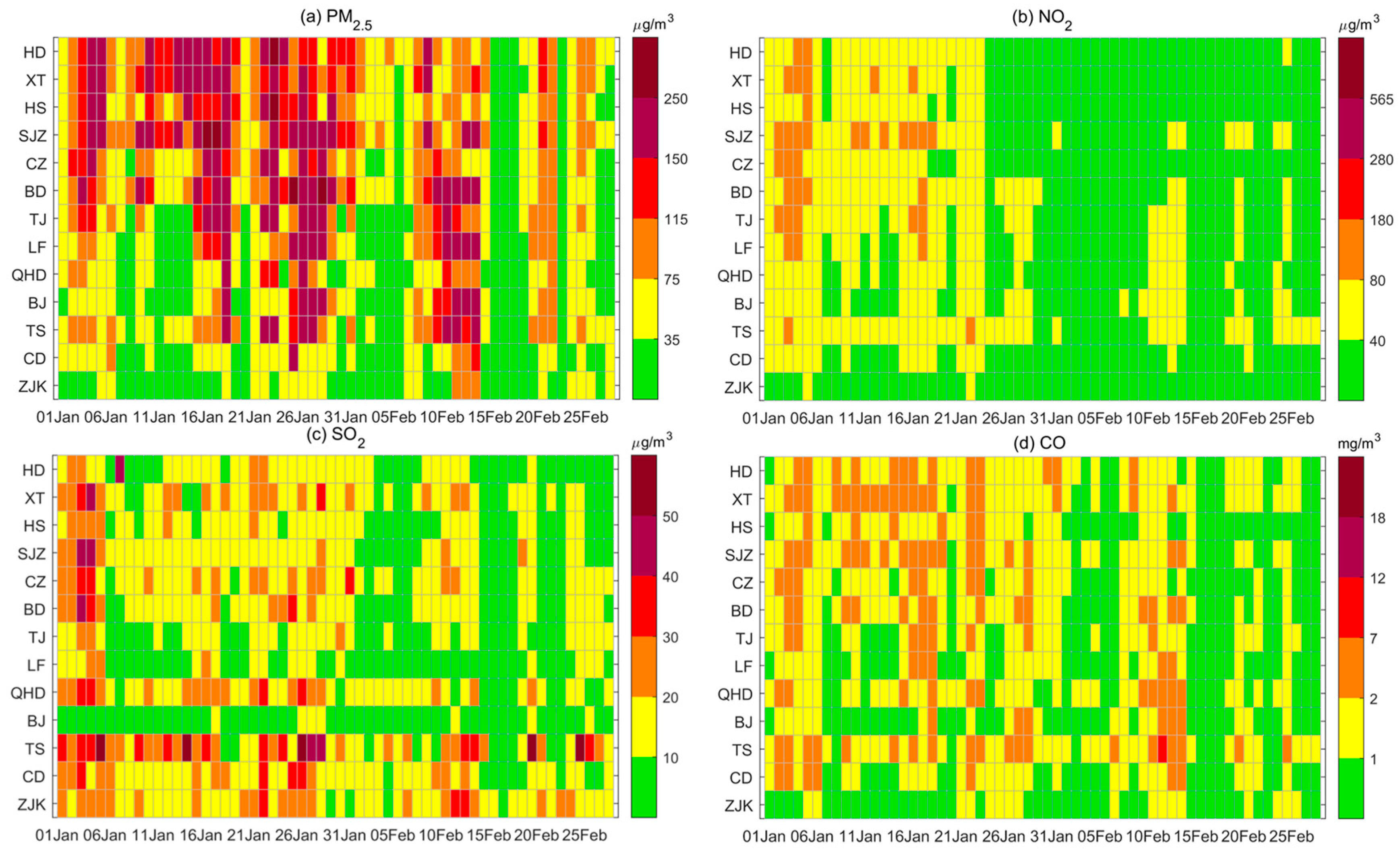
To understand the general variation characteristics of the pollutant concentration in the BTH region during the period, we first examined the concentrations of PM2.5, SO2, NO2 and CO in the 13 cities during the period January to February (Figure 2), respectively. Firstly, combined with the spatial distribution of the 13 cities in BTH, it is shown that the high concentrations were mainly concentrated in central and southern BTH in both January and February. Secondly, from the perspective of day-by-day variations, most of the cities in BTH region had a significant decrease in pollutant concentrations in February compared with January, especially the concentration of PM2.5 (Figure 2a) and NO2 (Figure 2b). Among them, the concentration of NO2 decreased the most, reaching −48.0%. As far as daytime and nighttime are concerned, the percentage or magnitude of pollutant concentration changes in February is roughly the same as that in January, although there are some differences or exceptions (Table 2). One exception, for example, is that the PM2.5 concentration in Beijing in February 2020 was slightly higher than that in January. In addition, both of PM2.5 and CO concentrations in Zhangjiakou in February 2020 were higher than those in January. These might be attributed to the heavy pollution caused by adverse weather conditions, which are conducive to the accumulation of pollutants and the formation of secondary aerosols and then causing an increase in PM2.5.
Generally, despite some differences existing in the spatial distribution and magnitude range of change, the mean PM2.5 and other pollutant concentrations in both daytime and nighttime dropped dramatically in February due to the strict quarantine or lockdown amid the outbreak of COVID-19. This is consistent with the results of other studies [27,28]. Therefore, the significant decrease of air pollutants in the BTH region in February 2020 compared with January can be considered as an unexpected change.
For an operational NWP system, the great difference of aerosol concentration in a short time constitutes the different background conditions. Next, we will examine whether it can cause some variation of the temperature prediction skills based on the regional NWP system of RMAPS and the global NWP system of ECMWF.

3.2. Differences in Temperature Forecast Skills between January and February 2020

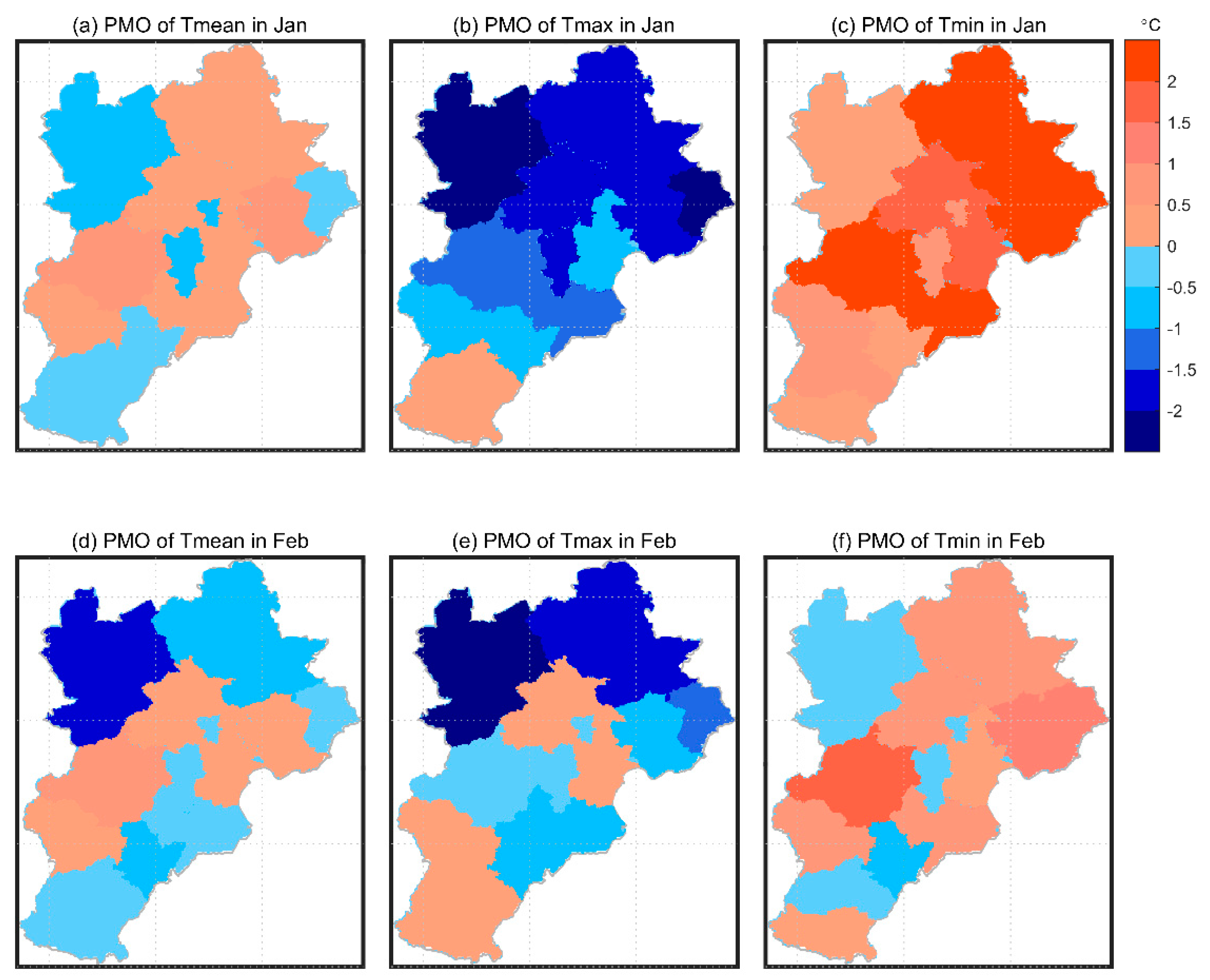
Figure 3 examines the average PMO of the daily mean temperature (Tmean), maximum temperature (Tmax) and minimum temperature (Tmin) with the forecast lead of 24 h (24 h for short) at the 13 cities in BTH in January and February. In January, the spatial distribution of Tmean PMO showed large spatial variability (Figure 3a); Tmax was generally underestimated except at the two southernmost cities (Figure 3b) while Tmin was overestimated at all 13 cities (Figure 3c). Concretely, the PMO of Tmax in January varied from −2.17 to 0.23 °C with an average of −1.15 °C. In contrast, the PMO of Tmin in January varied from 0.06 to 3.36 °C with an average of 1.46 °C.
In February, there was no distinct spatial consistency for the positive or negative bias of both Tmean, Tmax and Tmin (Figure 3d–f) prediction based on RMAPS. That is, the distinct systematic bias shown in the temperature prediction based on RMAPS model in BTH in January was markedly reduced in February, where the model bias was city dependent. Quantificationally, the PMO of Tmax (Tmin) in February varied from −2.91 (−0.61) to 0.20 (1.72) °C with an average of −0.62 (0.46) °C.
Table 2 presents the root mean square error (RMSE) between the predicted temperature and the observed temperature to eliminate the effect of bias signs. The RMSE of Tmean, Tmax and Tmin in January were 1.31 °C, 2.50 °C and 2.37 °C, respectively, while they were 1.08 °C, 2.26 °C and 1.86 °C in February. That is to say, the RMSE of the daily mean, maximum and minimum temperature prediction based on RMAPS model in BTH in February 2020 were 17.3%, 9.8% and 21.6% lower than that in January. Generally, the absolute deviation and the RMSE of the maximum and minimum temperature prediction in February were smaller than those in January. Moreover, for the forecasts with longer lead time (i.e., 48 h and 72 h forecast in advance), this feature is still evident (Table 2).
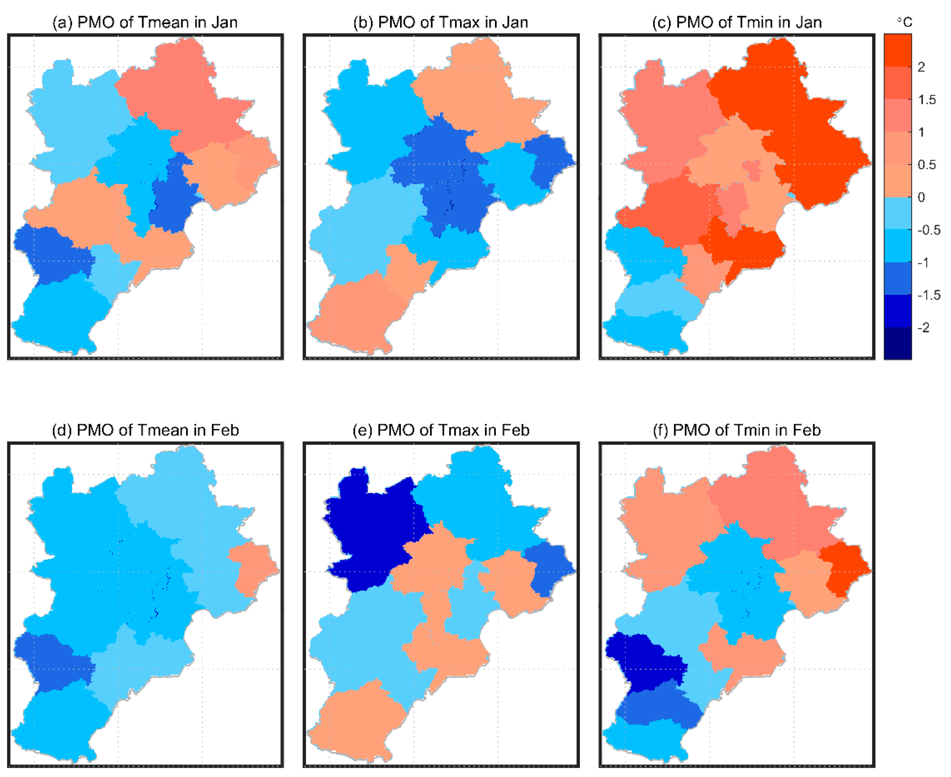
The PMO of Tmean, Tmax and Tmin in the 24 h forecast at the 13 cities in BTH in January and February based on the EC model was also examined. As shown in Figure 4, the systematic forecast bias of Tmax in January based on the EC model is quite different from that based on the RMAPS model. However, the overestimation of Tmin in January is in agreement with RMAPS, except for the underestimation of several cities in the south. Statistically, the RMSEs of Tmean, Tmax and Tmin based on the EC model were 1.08 °C, 2.02 °C and 2.09 °C in January, respectively, and then decreased to 0.88 °C, 1.73 °C and 1.65 °C in February (i.e., a reduction by 18.5%, 14.5% and 20.9%), respectively. As the forecast time extended to 48 and 72 h, this phenomenon was also still evident, although there are slight differences in degree (Table 2). That is, the distinct comparison characteristics of the bias and RMSE in the two months are generally consistent with those in the RMAPS model.
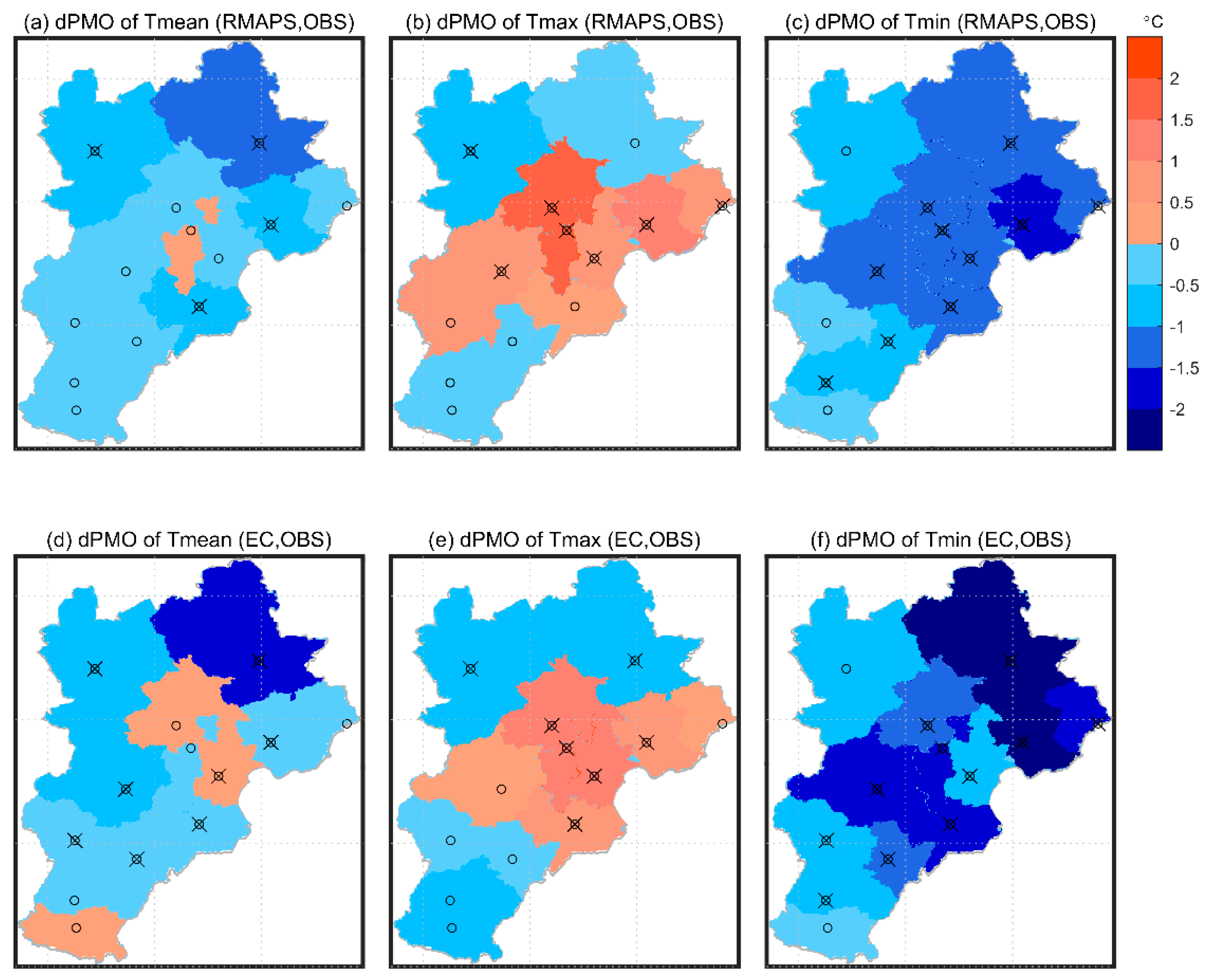
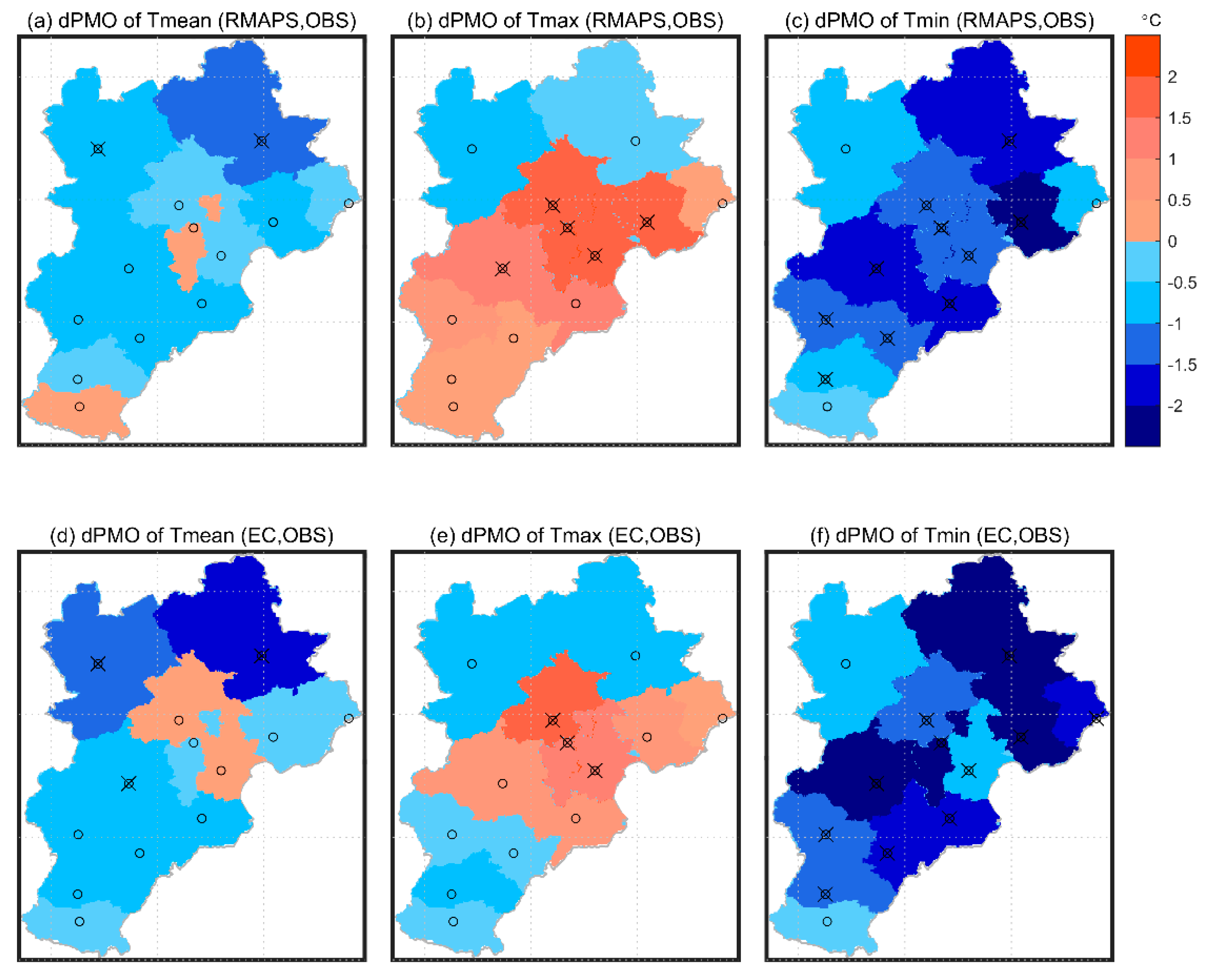
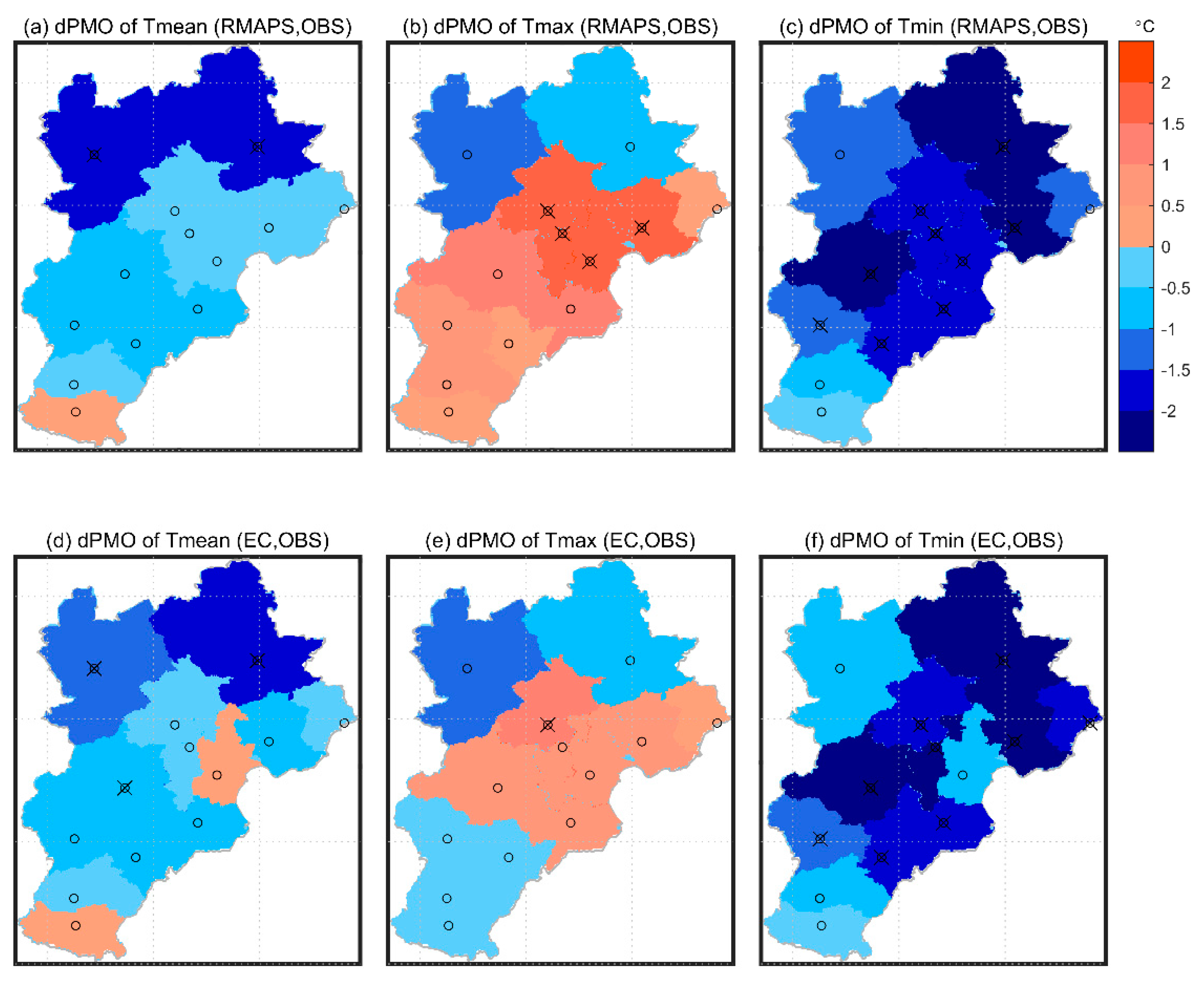
In order to better understand the NWP performance change of temperature forecast skills in February 2022 relative to that in January and its physical significance, we further examined the dPMO of the Tmean, Tmax and Tmin with the forecast lead of 24 h (Figure 5), 48 h (Figure 6), and 72 h (Figure 7) based on both the RMAPS and EC models. First of all, it can be seen that all cities are dominated by negative dPMO of Tmin in the BTH region, and most of them are significant at 95% confidence level (Figure 5c). However, most of the cities in BTH are covered by the positive dPMO of Tmax (Figure 5b). For the mean temperature, almost all the cities are featured by negative dPMO (Figure 5a), but the absolute values are generally lower than that in the minimum temperature. The negative (positive) dPMO indicates that the PMO in February is smaller (larger) than that in January, namely the RMAPS-based temperature forecast deviation was decreased (increased) in February.
On the other hand, the obvious difference between Figure 3 and Figure 5 is that the PMO of Tmin in the whole BTH region is positive (Figure 3c), while the dPMO of Tmin is negative (Figure 5c). As mentioned above, the positive of PMO in Figure 3 suggests that the RMAPS model overestimated the minimum temperature in January. Thus, the negative value of dPMO in Figure 5c indicates that, compared with January, the overestimation of the Tmin by RMAPS was decreased significantly in February. That is, the prediction skill of daily minimum temperature in February based on RMAPS has been improved. Meanwhile, the prediction of Tmax based on RMAPS in BTH in January was basically underestimated (Figure 3b) and was improved generally in February, especially in the central part of BTH region (Figure 5b). The spatial distribution characteristics and the comparisons of PMO and dPMO are basically similar when the forecast lead increases to 48 h (Figure 6) and 72 h (Figure 7).
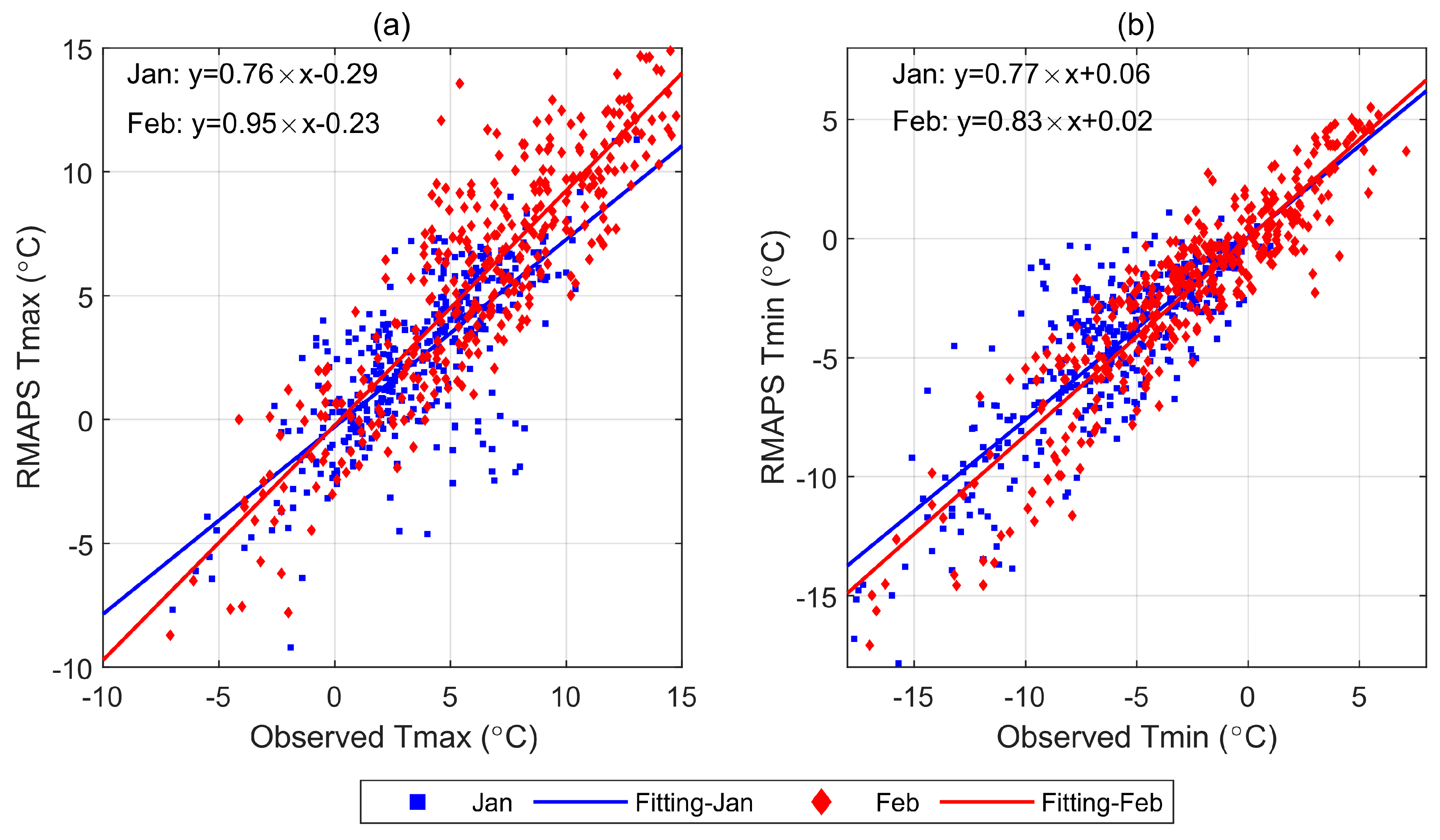
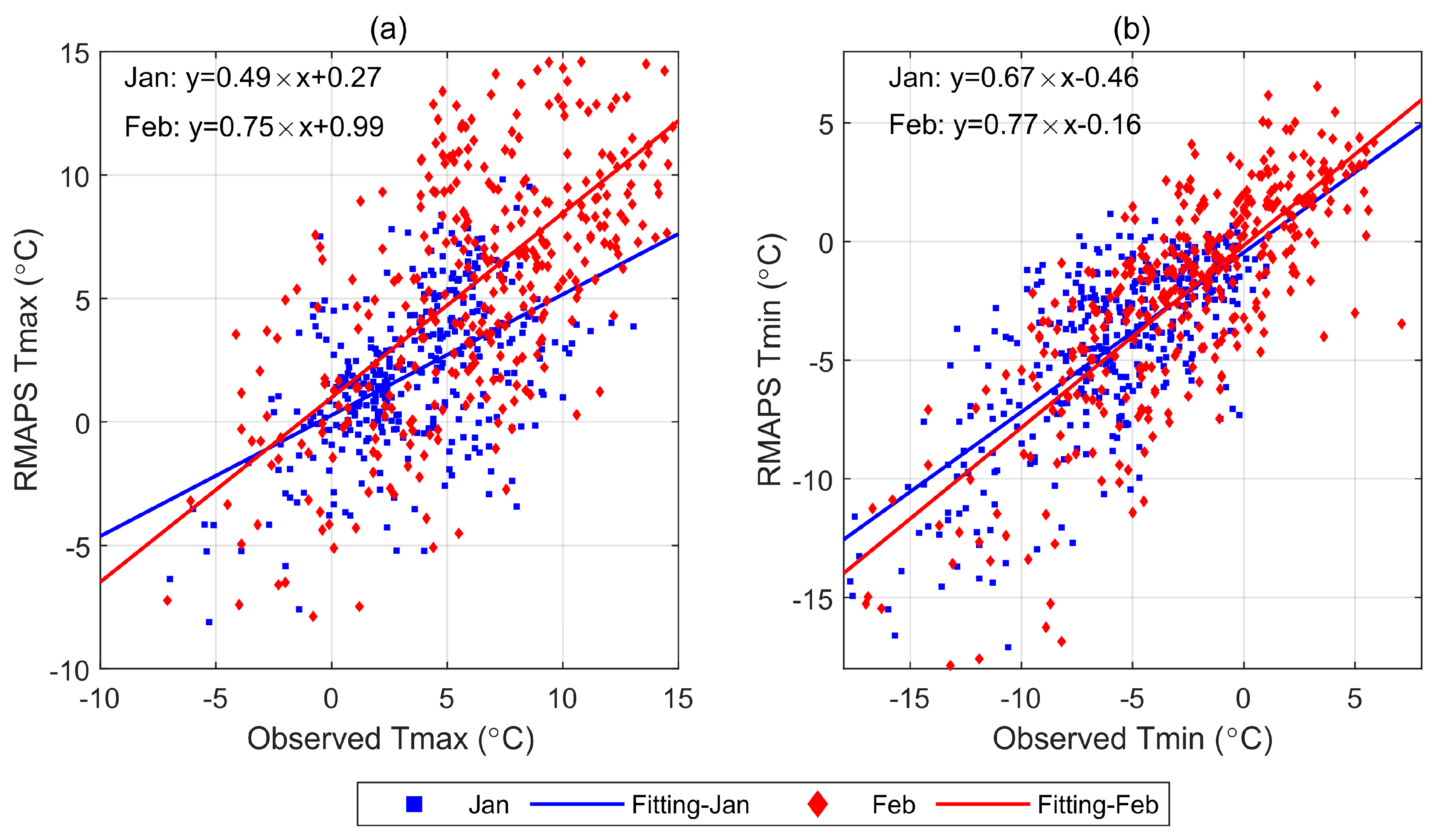
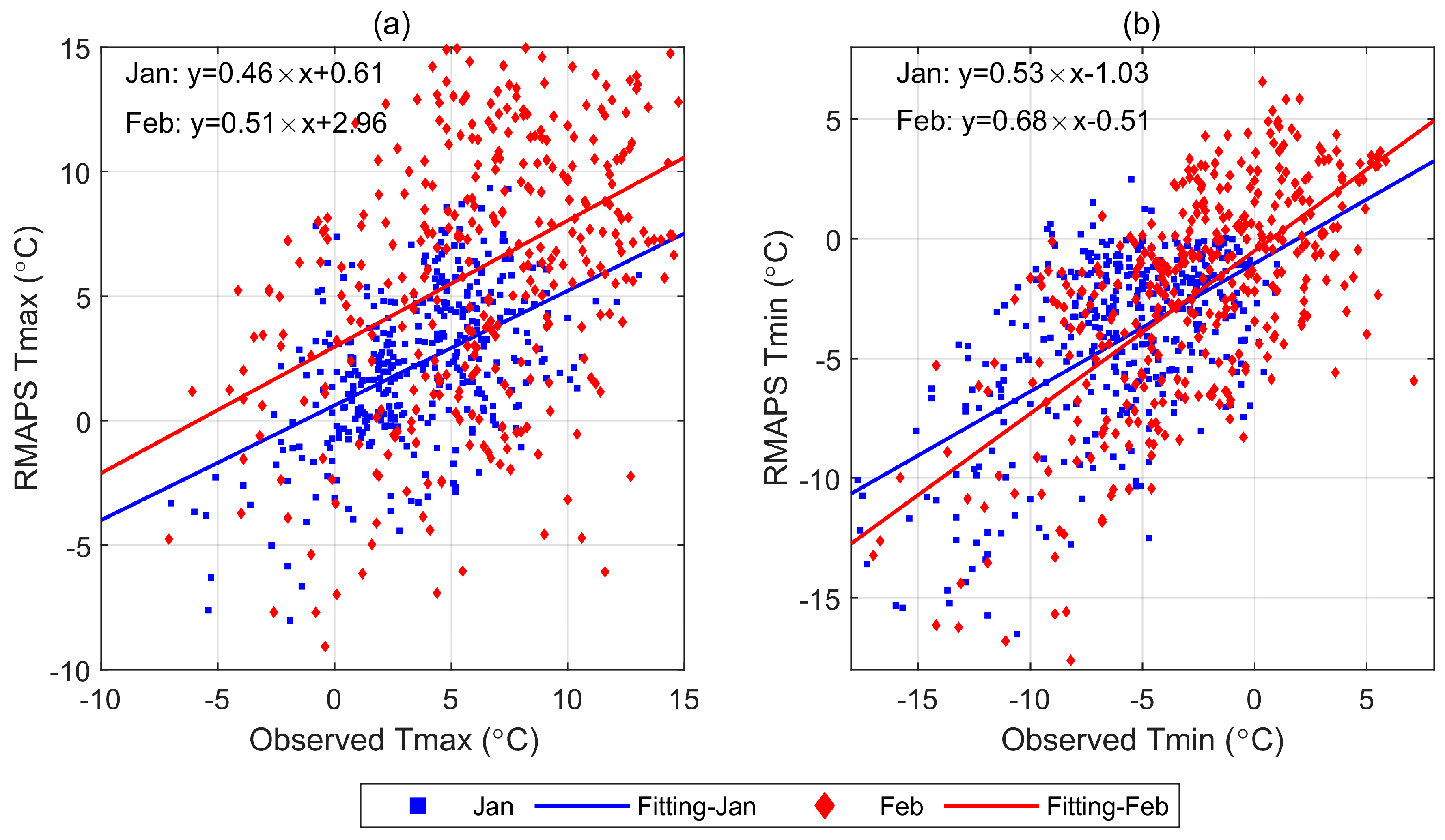
Figure 8, Figure 9 and Figure 10 further examine the difference of forecast skills of Tmax and Tmin in BTH in January and February based on RMAPS using scatter diagrams and fitting equations. It can be seen that, in both January and February, the dispersion of forecast and observation increased with the extension of the forecast lead time. That is to say, with the extension of the forecast lead time, the forecast skills of the model for both Tmax and Tmin were generally decreased. However, it can be quantitatively known from the fitting equations whether Tmax or Tmin and the regression coefficients in February are closer to 1 and greater than those of January. Taking Tmin as an example, for the forecast lead of 24 h, 48 h and 72 h, the regression coefficients of the fitting equation in February are 0.83, 0.77 and 0.68, respectively, significantly larger than the counterparts in January (0.77, 0.67 and 0.53). This undoubtedly shows that the forecast skill of the RMAPS model for the daily maximum and minimum temperatures in the region in February was better than that in January.
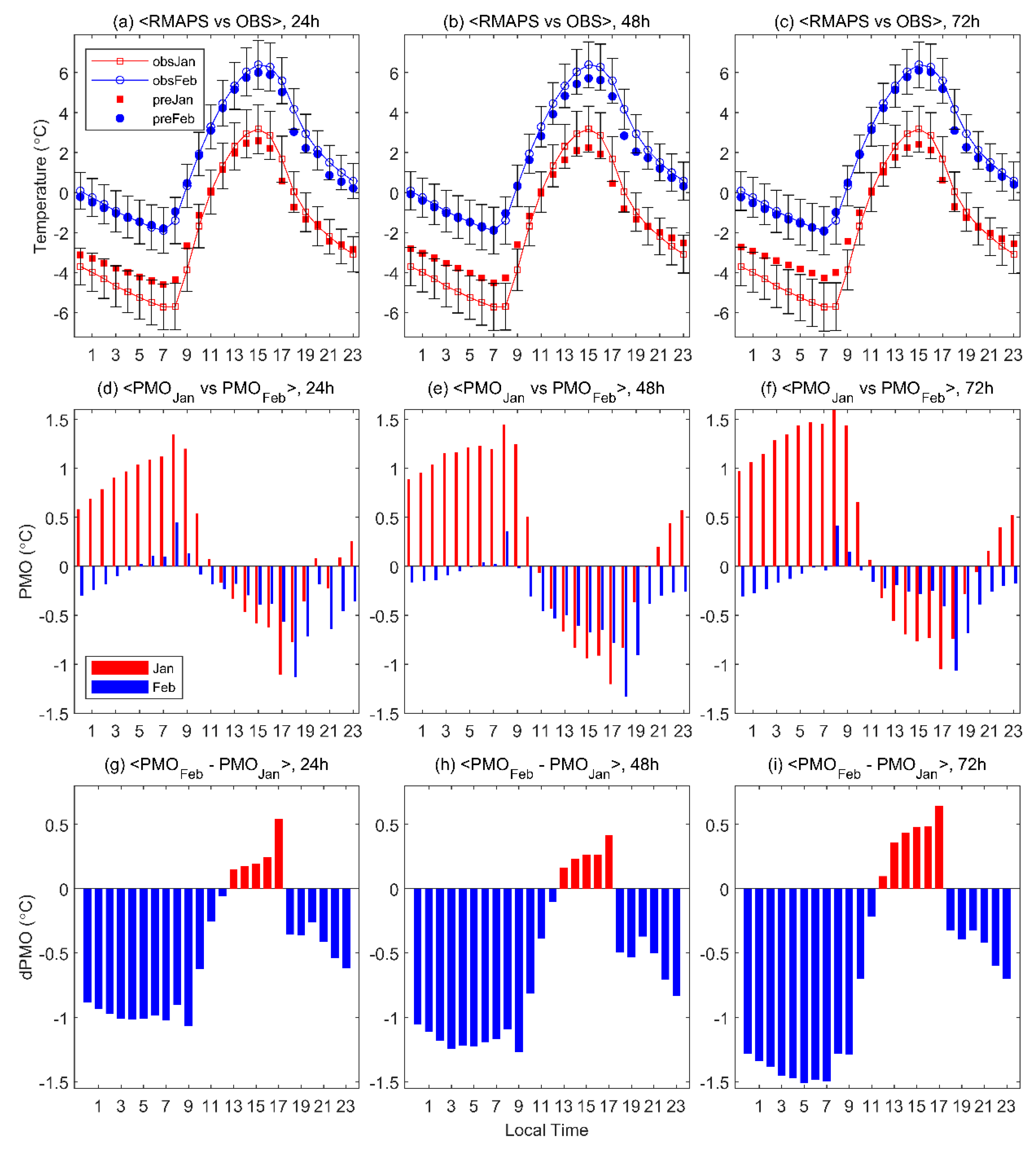
We also examine the model’s forecast performance of the temperature diurnal variation in January and February. Firstly, the observed and RMAPS-predicted temperature diurnal variations averaged over the 13 cities in BTH in January and February are presented for different forecast lead times in Figure 11a, Figure 11b and Figure 11c, respectively. Shown in Figure 11a, an obvious feature is that the RMAPS forecast temperature in January was significantly higher at 0–10 a.m. (local time) and lower at 1–7 p.m. than the observation. In contrast, the forecast and observed temperature diurnal variations in February are intuitively consistent, and the deviations at all times are much smaller than those in January. With the extension of the forecast lead (Figure 11b,c), although there is a slight difference in the magnitude of the specific changes, this phenomenon was still evident.
The second row in Figure 11 shows the diurnal variation of PMO (Tprediction − Tobservation) in January and February at the different forecast lead times. It is clear that the RMAPS model overestimated the nighttime temperature and underestimated the daytime temperature in January. The turning points were around 11 o’clock in the morning and 20 o’clock in the night, respectively. In February, the RMAPS model mainly underestimated the average temperature of the 13 cities throughout the day, with only a few positive deviations around 9 o’clock in the morning. The deviation mode in February is significantly different from that in January. It is worth noting that the absolute deviation of the temperature forecast in February is much smaller than that in January, especially at night.
Meanwhile, it is interesting to note that, regardless of whether the forecast period is 24 h, 48 h, or 72 h, the positive dPMO only appeared from 13 to 17 or 18 o’clock in the afternoon, and the rest was dominated by negative dPMO. Here, the positive values reflect the improvement of the underestimation of the daytime temperature forecast, while negative values indicate the improvement of the overestimation of the nighttime temperature forecast. That is, the diurnal variation characteristics of dPMO also suggested that the forecast skill of the RMAPS model for temperature over the BTH region in February was significantly improved than that in January. These results are basically consistent with those based on the EC model.
Based on the differences in bias, RMSE, spatial distribution and diurnal variation characteristics of the temperature forecast in January and February over the BTH region, it can be concluded that the temperature prediction skills in the BTH region, based on both RMAPS and EC models, were generally improved in February 2020 compared with those in January, especially for the minimum temperature prediction in nighttime, although the changes are model- and city-dependent to some extent. In order to understand the possible association between the improved temperature prediction skills and the reduced aerosol pollution, the changes and climatology characteristics of temperature, relative humidity, wind speed, cloud cover in January and February in BTH are discussed in the following.

4. Discussion

Why did the NWP performance in the temperature forecast over the BTH region differ greatly between January and February 2020? Generally speaking, in a relatively short period, without major upgrades or changes in an operational NWP system, the ability to predict a certain meteorological element should be basically the same. The significant change in the forecast skill might be related to the abnormal external influence. Therefore, it is necessary to explore whether this phenomenon is related to the response of meteorological conditions to the unexpected and significant changes in air pollutant concentrations.
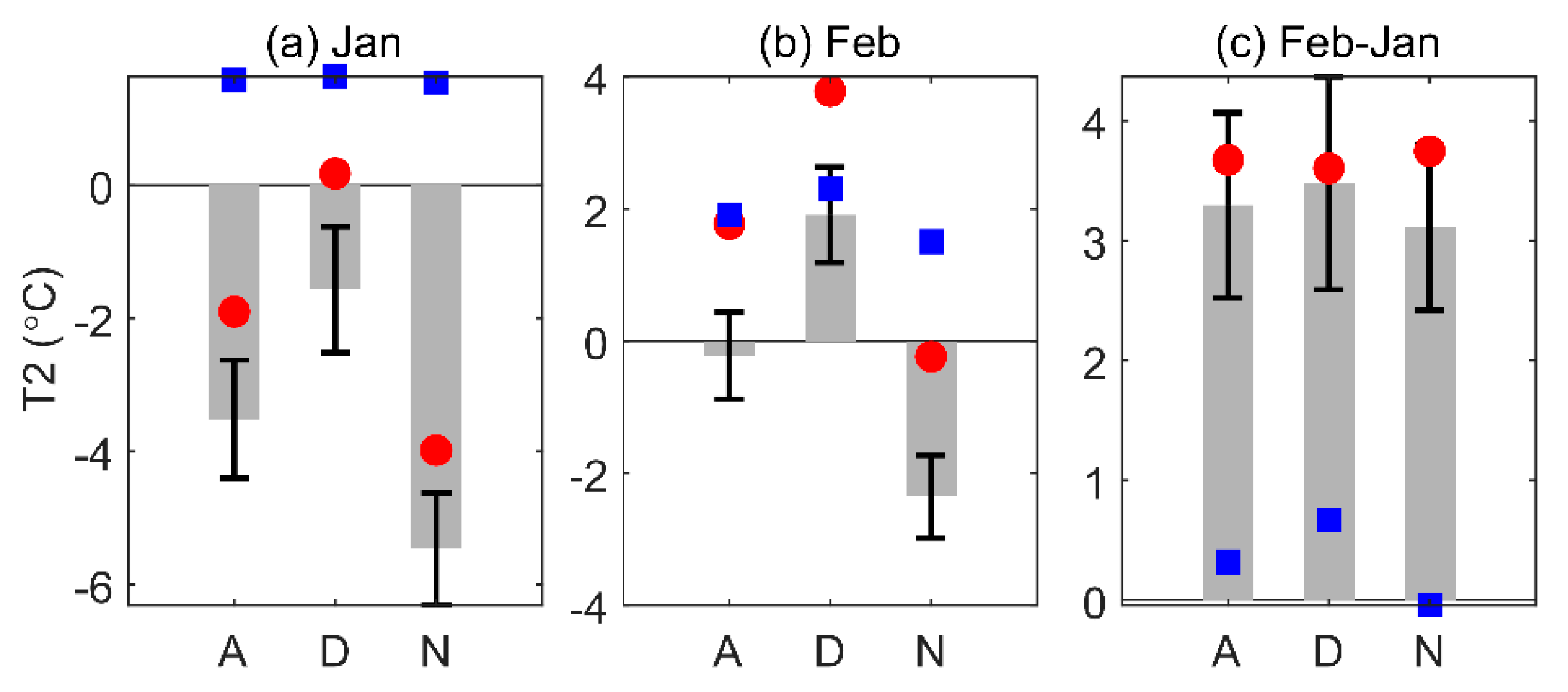
Figure 12 examines the mean air temperature at 2 m (T2) of January and February in 2020 and 2010–2019 and their differences are based on the hourly observations at the 44 synoptic meteorological stations located in the 13 cities. Whether in all day time (A), daytime (D) or nighttime (N), the climatological temperature in February and the temperature in February 2020 are higher than that of January. For the climatological temperature, the mean daytime (nighttime) T2 in January is −1.6 (−5.5) °C with the standard deviation of 1.9 (1.7) °C; while the mean daytime (nighttime) T2 in February is 1.9 (−2.4) °C with the standard deviation of 1.4 (1.3) °C, respectively. For the temperature in 2020, the mean daytime and nighttime T2 were 0.2 and −4.0 °C in January, and 3.8 and −0.2 °C in February, respectively. The increase of the monthly mean temperature in February relative to January is a climatic feature due to the seasonal variations of the solar radiation. On the other hand, both daytime and nighttime temperatures in January and February 2020 are significantly higher than the climatic means, which is likely to be attributed to the background of global and regional climate warming.
Therefore, it is necessary to exclude the effects of seasonal variations and climate warming when examining the differences of the temperature anomalies in January and February. Concretely, the anomaly daytime T2 of January and February 2020 were 1.63 and 2.30 °C, respectively, while the anomaly nighttime T2 of January and February 2020 were 1.54 and 1.50 °C, respectively. The anomaly daytime T2 deviation from February to January in 2020 was 0.67 °C, and the anomaly nighttime T2 deviation from February to January in 2020 was −0.04 °C.
The variations of the temperature anomaly in February and January are probably related to the changes in synoptic-scale weather factors, including relative humidity (RH), wind speed (WS), cloud cover (CLOCov), as well as chemical composition of the atmosphere. In addition, the variation of surface ground temperature in January and February 2020 also showed the similar comparative characteristics. The relatively high daytime temperature anomaly in February 2020 is likely related to the significant reduction of air pollutant concentration caused by epidemic controls [27,29]. A possible mechanism is that, the improvement of air quality largely means the decrease of aerosol concentration (i.e., PM2.5) in the atmosphere and thus less scattering and reflection of solar shortwave radiation, which is conducive to the increase of near-surface temperature. Although the temperature anomaly at night in February changed little compared with that in January, only −0.04 °C, it seemed to be consistent with the interaction mechanism of air pollution and temperature. Due to the decrease of aerosols, the blocking and absorption effects of the near-surface atmosphere on the outgoing longwave radiation (OLR) from ground at night will be weakened, thus reducing the ground temperature at night.
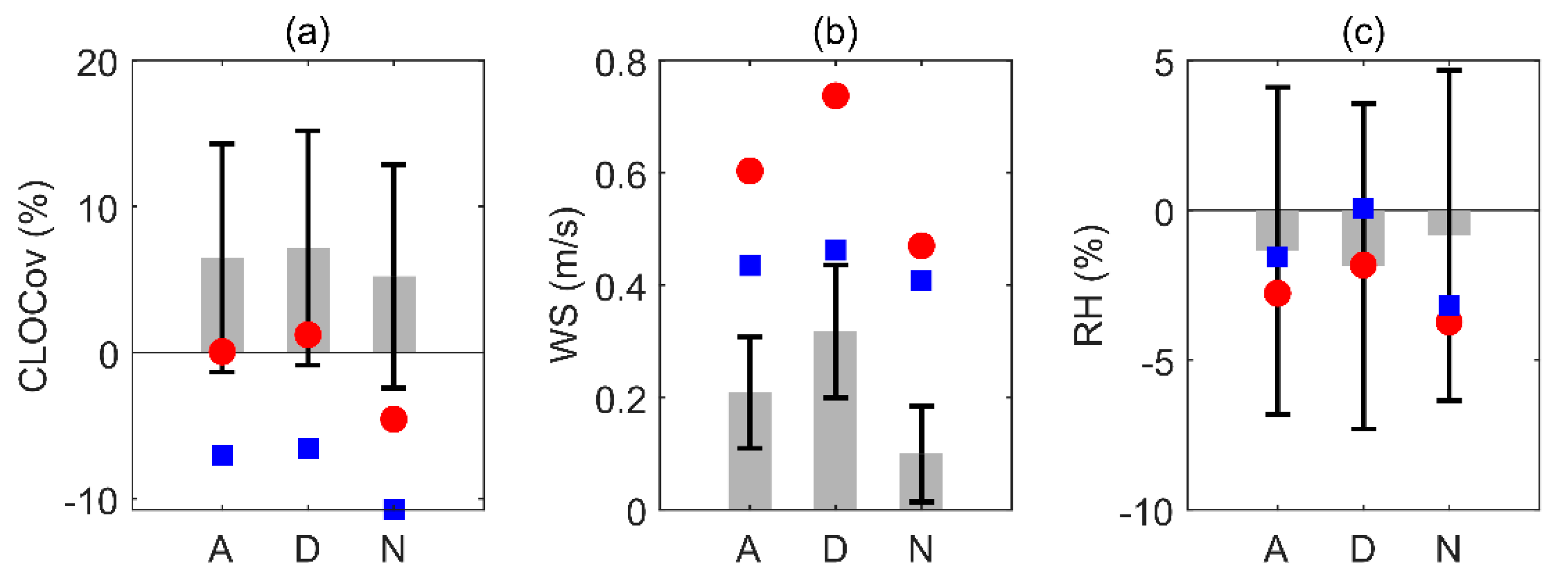
The anomaly of temperature may also be related to relative humidity, wind speed, cloud cover, and other factors. Here, the variations of RH, WS, and CLOCov in daytime and nighttime in January and February are also examined, respectively. In terms of the climatological statistics, the daytime RH in February in BTH is lower than that in January, and the change at night is not obvious; and both the daytime and nighttime WS and CLOCov in February were higher than those in January (gray bars in Figure 13).
As for the actual observed cloud cover in 2020, the cloud cover was slightly larger during the daytime and smaller during the nighttime in February than that in January (red dots in Figure 13). However, from the comparison of monthly anomalies (blue squares in Figure 13), the daytime clouds and night clouds in February 2022 were obviously fewer than those in January 2020. The possible mechanism of the cloud on the surface temperature is likely consistent with that of aerosols-temperature relations, although there are a lot of uncertainties in aerosol and cloud feedbacks [35,36]. Moreover, the increases of northerlies in nighttime and southerlies in daytime can cause a cooling in nighttime and warming in daytime, respectively (Figure 13b). And a reduction of RH in nighttime can be also beneficial to the increase of OLR and the surface cooling (Figure 13c).
Generally, the anomalous warming in daytime and cooling in nighttime in February 2020 are well consistent with changes of aerosol and meteorological factors in BTH, although the causal relationship between temperature variability and meteorological conditions is complex and highly uncertain. In theory, the effects of air pollutant concentrations on temperature can be achieved by an online-coupling meteorology–chemistry model, such as the WRF-Chem. Therefore, based on the online-coupling meteorology–chemistry model and the near authentic pollutant emission data, and with the assimilation of aerosol or not, a series of sensitivity numerical simulations are required to uncover the possible mechanism behind this phenomenon and improve the temperature forecasting skills.

5. Conclusions

Due to the strict industrial production and transportation restrictions and quarantines amid the outbreak of coronavirus disease (COVID-19), the air pollutant concentrations in BTH significantly dropped in February 2020 compared with that in January. This study is to explore whether this sudden significant background change will affect the NWP performance prediction. Based on a large number of air quality and meteorological observations, as well as the forecast data derived from a regional (RMAPS) and global (ECMWF) real-time operational NWP models, a series of quantitative and qualitative analyses were performed. The main conclusions are summarized as follows.
(1) The air pollutant concentrations over the BTH in February 2020 were dramatically lower than that in January. For example, the concentrations of PM2.5 and NO2 were decreased by 38.5% and 48.0%, respectively. Simultaneously, after removing the climatological signal, the BTH region experienced an anomalous warming in daytime and an anomalous cooling in nighttime in February, respectively. The warming and cooling trends are generally consistent with changes of cloud cover, wind speed and relative humidity.
(2) The forecast performance of NWP models for daily maximum (Tmax) and minimum (Tmin) temperature over the BTH in February 2020 was significantly improved compared with that in January. In 24 h forecast lead time in advance, the root mean square errors (RMSE) of Tmax and Tmin prediction based on RMAPS in February were 9.8% and 21.6% lower than those in January, respectively. This phenomenon basically existed when the forecast lead time extended to 48 h and 72 h. And a similar result was also presented in the operational global ECMWF model.
(3) It is suggested that the temperature forecasting skill based on NWP models in February 2020 was generally improved, and this might be partly attributed to the significant reduction of aerosol pollutant concentrations in a short period of time, although the specific effect of aerosols on temperature prediction is likely to be regional- and model-dependent. The possible links deduce that less aerosols in daytime are beneficial to more solar radiation and a warming in the near-surface temperature. Contrarily, less aerosols in nighttime are not conducive to stop the outgoing long-wave radiation and lead to a cooling near the ground. The response mechanism of these meteorological conditions to the changes of aerosol concentrations is likely to be the reason for the improvement of NWP model’s temperature prediction skills in February. Therefore, a further study with a series of sensitivity numerical simulations based on an online-coupling meteorology–chemistry model is warranted for better understanding of the detailed mechanism.

Author Contributions

Conceptualization, Z.Z. and Y.L.; methodology, Z.Z.; software, S.C.; validation, Y.L., and S.C.; formal analysis, Z.Z.; investigation, S.C.; resources, Z.Z.; data curation, Z.Z.; writing—original draft preparation, Z.Z.; writing—review and editing, S.C.; visualization, Y.L.; supervision, Z.Z.; project administration, Z.Z.; funding acquisition, Z.Z. All authors have read and agreed to the published version of the manuscript.

Funding

This study was supported by the National Natural Science Foundation of China (grant no. 41975168, 42175188), and by Beijing Municipal Natural Science Foundation (grant no. 8222049).

Institutional Review Board Statement

Not applicable.

Informed Consent Statement

Not applicable.

Data Availability Statement

The datasets are available upon request.

Conflicts of Interest

The authors declare no conflict of interest.

References

  1. Zhang, Y.; Chen, X.; Yu, S.; Wang, L.; Li, Z.; Li, M.; Liu, W.; Li, P.; Rosenfeld, D.; Seinfeld, J.H. City-level air quality improvement in the Beijing-Tianjin-Hebei region from 2016/17 to 2017/18 heating seasons: Attributions and process analysis. Environ. Pollut. 2021, 274, 116523. [Google Scholar] [CrossRef]
  2. Luo, Y.H.; Zhao, T.L.; Yang, Y.J.; Zong, L.; Kumar, K.P.; Wang, H.; Meng, K.; Zhang, L.; Lu, S.; Xin, Y.S. Seasonal changes in the recent decline of combined high PM2.5 and O3 pollution and associated chemical and meteorological drivers in the Beijing–Tianjin–Hebei region. China Sci. Total Environ. 2022, 838, 156312. [Google Scholar] [CrossRef]
  3. Liu, Y.; Tian, J.W.; Zheng, W.F.; Yin, L.R. Spatial and temporal distribution characteristics of haze and pollution particles in China based on spatial statistics. Urban Clim. 2022, 41, 101031. [Google Scholar] [CrossRef]
  4. National Bureau of Statistics of China. China Statistical Yearbook (2021); China Statistics Press: Beijing, China, 2021. [Google Scholar]
  5. Gao, M.; Liu, Z.R.; Zheng, B.; Ji, D.S.; Sherman, P.; Song, S.J.; Xin, J.Y.; Liu, C.; Wang, Y.S.; Zhang, Q.; et al. China’s emission control strategies have suppressed unfavorable influences of climate on wintertime PM2.5 concentrations in Beijing since 2002. Atmos. Chem. Phys. 2020, 20, 497–1505. [Google Scholar] [CrossRef] [Green Version]
  6. Zhang, Z.Y.; Zhao, X.J.; Mao, R.; Xu, J.; Kim, S.J. Predictability of the winter haze pollution in Beijing–Tianjin–Hebei region in the context of stringent emission control. Atmos. Pollut. Res. 2022, 13, 101392. [Google Scholar] [CrossRef]
  7. Zhao, N.; Elshareef, H.; Li, B.W.; Wang, B.M.; Jia, Z.Z.; Zhou, L.; Liu, Y.; Sultan, M.; Dong, R.J.; Zhou, Y.G. The efforts of China to combat air pollution during the period of 2015–2018: A case study assessing the environmental, health and economic benefits in the Beijing-Tianjin-Hebei and surrounding “2 + 26” regions. Sci. Total Environ. 2022, 853, 158437. [Google Scholar] [PubMed]
  8. Zhang, Z.Y.; Zhang, X.L.; Gong, D.Y.; Kim, S.J.; Mao, R.; Zhao, X.J. Possible influence of atmospheric circulations on winter hazy pollution in Beijing-Tianjin-Hebei region, northern China. Atmos. Chem. Phys. 2016, 16, 561–571. [Google Scholar] [CrossRef] [Green Version]
  9. Zhai, S.X.; Jacob, D.J.; Wang, X.; Shen, L.; Li, K.; Zhang, Y.Z.; Gui, K.; Zhao, T.L.; Liao, H. Fine particulate matter (PM2.5) trends in China, 2013–2018: Separating contributions from anthropogenic emissions and meteorology. Atmos. Chem. Phys. 2019, 19, 11031–11041. [Google Scholar]
  10. Kumar, R.P.; Perumpully, S.J.; Samuel, C.; Gautam, S. Exposure and health: A progress update by evaluation and scientometric analysis. Stoch. Environ. Res. Risk Assess. 2023, 37, 453–465. [Google Scholar]
  11. Yin, L.; Wang, L.; Huang, W.; Tian, J.; Liu, S.; Yang, B.; Zheng, W. Haze Grading Using the Convolutional Neural Networks. Atmosphere 2022, 13, 522. [Google Scholar] [CrossRef]
  12. Intergovernmental Panel on Climate Change (IPCC). Climate Change 2021: The Physical Science Basis; Cambridge University Press: Cambridge, UK, 2021. [Google Scholar]
  13. Wang, Y.; Khalizov, A.; Zhang, R. New directions: Light absorbing aerosols and their atmospheric impacts. Atmos. Environ. 2013, 81, 713–715. [Google Scholar]
  14. Ding, A.J.; Huang, X.; Nie, W.; Sun, J.N.; Kerminen, V.M.; Petäjä, T.; Su, H.; Cheng, Y.; Yang, X.Q.; Wang, M.; et al. Enhanced haze pollution by black carbon in megacities in China. Geophys. Res. Lett. 2016, 43, 2873–2879. [Google Scholar] [CrossRef]
  15. Li, Z.Q.; Guo, J.P.; Ding, A.J.; Liao, H.; Liu, J.J.; Sun, Y.L.; Wang, T.J.; Xue, H.W.; Zhang, H.S.; Zhu, B. Aerosol and boundary-layer interactions and impact on air quality. Natl. Sci. Rev. 2017, 4, 810–833. [Google Scholar]
  16. Watson-Parris, D.; Bellouim, N.; Deaconu, L.T.; Schutgens, N.A.J.; Youshioka, M.; Regayre, L.A.; Pringle, K.J.; Johnson, J.S.; Smith, C.J.; Carslaw, K.S.; et al. Constraining uncertainty in aerosol direct forcing. Geophys. Res. Lett. 2020, 47, e2020GL087141. [Google Scholar] [CrossRef]
  17. Kumar, R.P.; Brema, J.; Samuel, C.; Gautam, S. A bibliometric and scientometric: Analysis towards global pattern and trends related to aerosol and precipitation studies from 2002 to 2022. Air Qual. Atmos. Health 2023, 16, 613–628. [Google Scholar]
  18. Hohenegger, C.; Vidale, P.L. Sensitivity of the European climate to aerosol forcing as simulated with a regional climate model. J. Geophys. Res. 2005, 110, D06201. [Google Scholar] [CrossRef]
  19. Zubler, E.M.; Lohmann, U.; Lüthi, D.; Schär, C. Intercomparison of aerosol climatologies for use in a regional climate model over Europe. Geophys. Res. Lett. 2011, 38, L15705. [Google Scholar] [CrossRef]
  20. Makar, P.A.; Gong, W.; Milbrandt, J.; Hogrefe, C.; Zhang, Y.; Curci, G.; Zabkar, R.; Im, U.; Balzarini, A.; Baro, R.; et al. Feedbacks between air pollution and weather, Part I: Effects on weather. Atmos. Environ. 2015, 115, 442–469. [Google Scholar]
  21. Makar, P.A.; Gong, W.; Hogrefe, C.; Zhang, Y.; Curci, G.; Zabkar, R.; Milbrandt, J.; Im, U.; Balzarini, A.; Baro, R.; et al. Feedbacks between air pollution and weather, Part II: Effects on chemistry. Atmos. Environ. 2015, 115, 499–526. [Google Scholar]
  22. de Perez, E.C.; van Aalst, M.; Bischiniotis, K.; Mason, S.; Nissan, H.; Pappenberger, F.; Stephens, E.; Zsoter, E.; van den Hurk, B. Global predictability of temperature extremes. Environ. Res. Lett. 2018, 13, 054017. [Google Scholar] [CrossRef]
  23. Benedetti, A.; Vitart, F. Can the direct effect of aerosols improve subseasonal predictability? Mon. Weather. Rev. 2018, 146, 3481–3498. [Google Scholar] [CrossRef]
  24. Choi, I.J.; Park, R.S.; Lee, J. Impacts of a newly-developed aerosol climatology on numerical weather prediction using a global atmospheric forecasting model. Atmos. Environ. 2019, 197, 77–91. [Google Scholar] [CrossRef]
  25. Jeong, G.R. Weather Effects of Aerosols in the Global forecast Model. Atmosphere 2020, 11, 850. [Google Scholar] [CrossRef]
  26. Huang, X.; Ding, A. Aerosol as a critical factor causing forecast biases of air temperature in global numerical weather prediction models. Sci. Bull. 2021, 66, 1917–1924. [Google Scholar] [CrossRef] [PubMed]
  27. Chen, Q.X.; Huang, C.L.; Yuan, Y.; Tan, H.P. Influence of COVID-19 Event on Air Quality and their Association in Mainland China. Aerosol Air Qual. Res. 2020, 20, 1541–1551. [Google Scholar] [CrossRef]
  28. Filonchyk, M.; Hurynovich, V.; Yan, H.; Gusev, A.; Shpilevskaya, N. Impact Assessment of COVID-19 on Variations of SO2, NO2, CO and AOD over East China. Aerosol Air Qual. Res. 2020, 20, 1530–1540. [Google Scholar] [CrossRef]
  29. Bauwens, M.; Compernolle, S.; Stavrakou, T.; Müller, J.-F.; Gent, J.; Eskes, H.; Levelt, P.F.; van der, A.R.; Veefkind, J.P.; Vlietinck, J.; et al. Impact of coronavirus outbreak on NO2 pollution assessed using TROPOMI and OMI observations. Geophys. Res. Lett. 2020, 47, e2020GL087978. [Google Scholar] [CrossRef]
  30. Tian, J.W.; Liu, Y.; Zheng, W.F.; Yin, L.R. Smog prediction based on the deep belief—BP neural network model (DBN-BP). Urban Clim. 2022, 41, 101078. [Google Scholar] [CrossRef]
  31. Xu, Z.; Liu, Z.; Tian, J.; Liu, Y.; Pan, H.; Liu, S.; Yang, B.; Yin, L.; Zheng, W. Classification of Urban Pollution Levels Based on Clustering and Spatial Statistics. Atmosphere 2022, 13, 494. [Google Scholar] [CrossRef]
  32. Shang, K.L.; Chen, Z.Y.; Liu, Z.X.; Song, L.H.; Zheng, W.F.; Yang, B.; Liu, S.; Yin, L.R. Haze Prediction Model Using Deep Recurrent Neural Network. Atmosphere 2021, 12, 1625. [Google Scholar] [CrossRef]
  33. Barker, D.; Huang, X.Y.; Liu, Z.; Auligné, T.; Zhang, X.Y.; Rugg, S.; Ajjaji, R.; Bourgeois, A.; Bray, J.; Chen, Y.; et al. The weather research and forecasting model’s community variational/ensemble data assimilation system: WRFDA. Bull. Am. Meteorol. Soc. 2012, 93, 831–843. [Google Scholar] [CrossRef] [Green Version]
  34. Xie, Y.H.; Fan, S.Y.; Chen, M.; Shi, J.C.; Zhong, J.Q.; Zhang, X.Y. An assessment of satellite radiance data assimilation in RMAPS. Remote Sens. 2019, 11, 54. [Google Scholar] [CrossRef] [Green Version]
  35. Ceppi, P.; McCoy, D.T.; Hartmann, D.L. Observational evidence for a negative shortwave cloud feedback in middle to high latitudes. Geophys. Res. Lett. 2016, 43, 1331–1339. [Google Scholar] [CrossRef] [Green Version]
  36. Zelinka, M.D.; Zhou, C.; Klein, S.A. Insights from a refined decomposition of cloud feedbacks. Geophys. Res. Lett. 2016, 43, 9259–9269. [Google Scholar] [CrossRef]
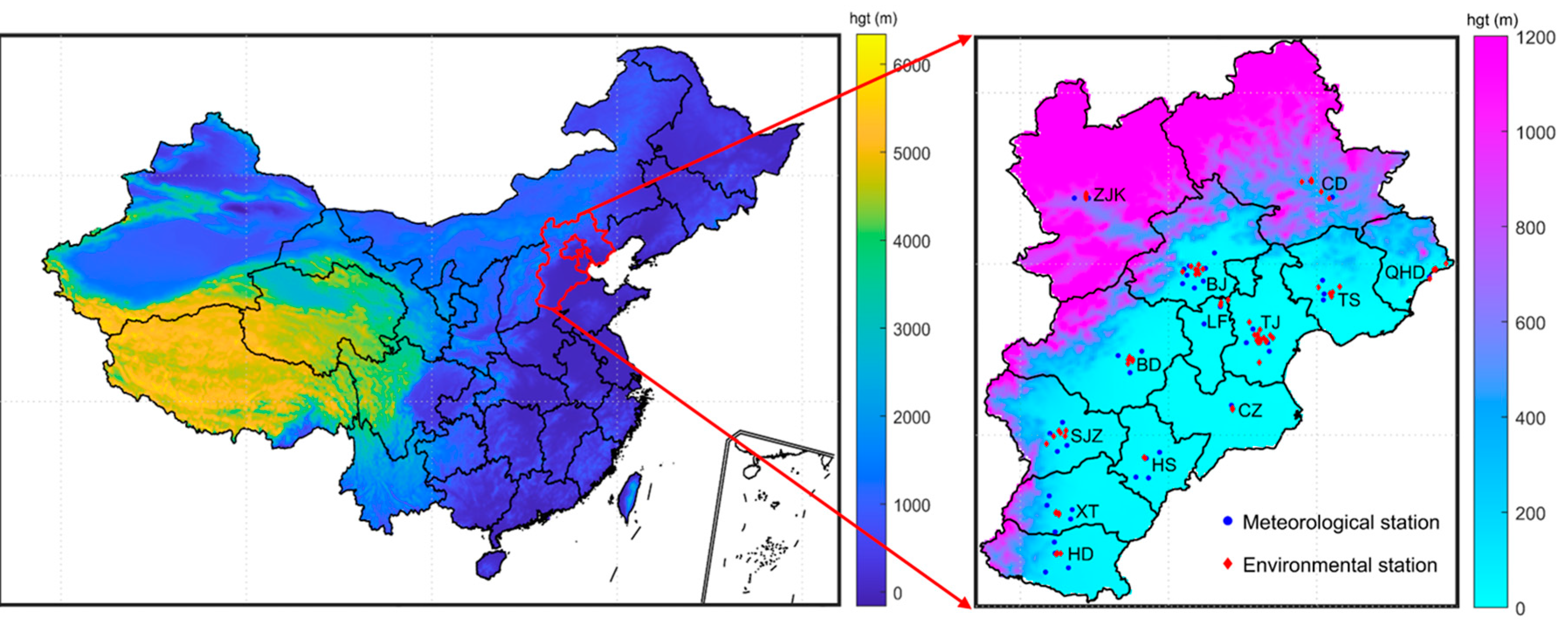
Figure 1. Locations of BTH region and meteorological and environmental stations in the 13 cities in BTH.
Atmosphere 14 01229 g001
Figure 2. The day-by-day variations of PM2.5 (a), NO2 (b), SO2 (c) and CO (d) concentrations in the 13 cities during 1 January to 28 February 2020.
Atmosphere 14 01229 g002
Figure 3. The PMO of the Tmean, Tmax and Tmin based on RMAPS in January (ac) and February (df) in 24 h forecast lead time in advance.
Atmosphere 14 01229 g003
Figure 4. The PMO of Tmean, Tmax and Tmin based on EC in January (ac) and February (df) in 24 h forecast lead time in advance.
Atmosphere 14 01229 g004
Figure 5. The dPMO of the Tmean, Tmax and Tmin derived from RMAPS (ac) and EC (df) in 24 h forecast lead time in advance (the circles represent the spatial position of the 13 cities; the cross markers denote 95% confidence level).
Atmosphere 14 01229 g005
Figure 6. The dPMO of the Tmean, Tmax and Tmin derived from RMAPS (ac) and EC (df) in 48 h forecast lead time in advance (same as Figure 5).
Atmosphere 14 01229 g006
Figure 7. The dPMO of the Tmean, Tmax and Tmin derived from RMAPS (ac) and EC (df) in 72 h forecast lead time in advance (same as Figure 5).
Atmosphere 14 01229 g007
Figure 8. Scatter plots of the observed Tmax (a) and Tmin (b) versus the predicted by RMAPS model in 24 h forecast lead time in advance.
Atmosphere 14 01229 g008
Figure 9. Scatter plots of the observed Tmax (a) and Tmin (b) versus the predicted by RMAPS model in 48 h forecast lead time in advance.
Atmosphere 14 01229 g009
Figure 10. Scatter plots of the observed Tmax (a) and Tmin (b) versus the predicted by RMAPS model in 72 h forecast lead time in advance.
Atmosphere 14 01229 g010
Figure 11. Diurnal variation of the temperature (ac) and PMO (df) and dPMO (gi) in BTH region based on the observation and RMAPS model (the error bars in a, b and c indicate the hourly standard deviation of 13 cities in BTH region).
Atmosphere 14 01229 g011
Figure 12. Then, mean T2 in January (a) and February (b) in 2020 (red dots) and their climatological values (grey histograms), and the differences of T2 in January and February (c) (A, D and N denote All day long, Daytime and Nighttime, respectively; Jan and Feb are abbreviations of January and February, respectively; Feb-Jan means the temperature difference between February and January; the red dots represent the temperature in 2020; the blue squares indicate the temperature anomaly of 2020 relative to the climatic state; the error bars of the gray histogram represent temperature variance of the 13 cities in BTH).
Atmosphere 14 01229 g012
Figure 13. Differences of CLOCov (a), WS (b) and RH (c) in February compared to January (the red circles represent the observations in 2020; the blue squares indicate the anomaly of 2020 relative to the climatic state; the error bars of the gray histogram represent variance of the 13 cities in BTH).
Atmosphere 14 01229 g013
Table 1. The monthly mean pollutant concentration and the percent change of that in February with respect to January.
JanuaryFebruaryPercentage
PM2.5All day long99.060.9−38.5%
Daytime93.457.4−38.6%
Nighttime104.664.4−38.4%
SO2All day long17.411.3−35.1%
Daytime18.512.0−35.3%
Nighttime16.310.6−34.9%
NO2All day long50.326.2−48.0%
Daytime45.622.7−50.2%
Nighttime55.129.7−46.2%
COAll day long1.611.08−33.1%
Daytime1.581.06−32.6%
Nighttime1.651.09−33.6%
Daytime indicates the hours from 8 a.m. to 19 p.m.; Nighttime indicates the time from 20 p.m. to 7 a.m.; all day long means all 24 h of each day; the unit of PM2.5, SO2 and NO2 is µg/m3 while the unit of CO is mg/m3.
Table 2. RMSE of the predicted Tmean, Tmax and Tmin against the observations in BTH region in January and February at different lead times.
RMAPS vs. OBS EC vs. OBS
January (°C)February (°C)Change* (%)January (°C)February (°C)Change (%)
24 hTmean1.311.08−17.31.080.88−18.5
Tmax2.502.26−9.82.021.73−14.5
Tmin2.371.86−21.62.091.65−20.9
48 hTmean2.652.19−17.42.331.95−16.3
Tmax3.843.38−12.03.593.05−15.0
Tmin3.322.68−19.32.752.25−18.1
72 hTmean3.773.25−13.83.383.07−9.3
Tmax4.544.05−10.85.104.65−8.8
Tmin3.623.02−16.53.353.02−9.7
(* indicate the percentage change of RMSE of temperature forecast in February relative to January).
Disclaimer/Publisher’s Note: The statements, opinions and data contained in all publications are solely those of the individual author(s) and contributor(s) and not of MDPI and/or the editor(s). MDPI and/or the editor(s) disclaim responsibility for any injury to people or property resulting from any ideas, methods, instructions or products referred to in the content.