Abstract
In recent years, the concentrations of PM2.5 in urban ambient air in China have been declining; however, the strong atmospheric oxidation capacity (AOC) represents challenges to the further reduction of PM2.5 concentration and the continuous improvement of ambient air quality in China in the future, since the overall AOC is still at a high level. For this paper, based on ground observation data recorded in Beijing from 2016 to 2019, the variation in AOC was characterized according to the concentration of odd oxygen (OX = O3 + NO2). The concentrations of the primary and secondary components of PM2.5 were analyzed using empirical formulas, the correlation between AOC and the concentrations of secondary PM2.5 and the secondary inorganic components (SO42−, NO3−, NH4+, and SNA) in Beijing were explored, the impact of atmospheric photochemical reaction activity on the generation of atmospheric secondary particles was evaluated, and the impact of atmospheric oxidation variations on PM2.5 concentrations and SNA in Beijing was investigated. The results revealed that OX concentrations reached their peak in 2016 and reached their lowest point in 2019. The OX concentrations followed a descending seasonal trend of summer, spring, autumn, and winter, along with a spatial descending trend from urban observation stations to suburban stations and background stations. The degree of photochemical activity and the magnitude of the AOC have a large influence on the production of atmospheric secondary particles. When the photochemical reaction was more active and the AOC was stronger, the mass concentrations of the secondary generated PM2.5 fraction were higher and accounted for a higher proportion of the total PM2.5 mass concentrations. In the PM2.5 fraction, SNA accounted for 50.7% to 94.4% of the total mass concentrations of water-soluble inorganic ions in the field observations. Higher concentrations of the atmospheric oxidant OX in ambient air corresponded to a higher sulfur oxidation ratio (SOR) and nitrogen oxidation ratio (NOR), suggesting that the increase in AOC could promote the increase of PM2.5 concentration. Based on a relationship analysis of SOR, NOR, and OX, it was inferred that the relationship between OX and SOR and the relationship between OX and NOR were both nonlinear. Therefore, when establishing PM2.5 control strategies in Beijing in the future, the impact of the AOC on PM2.5 generation should be fully considered, and favorable measures should be taken to properly regulate the AOC, which would be more effective when carrying out further control measures regarding PM2.5 pollution.
1. Introduction
In order to address its heavy air pollution, China has promulgated a series of national action plans since 2013, including the Air Pollution Prevention Scheme and the Control Action Plan, the Three-Year Action Plan for Blue Sky Protection Campaign, and the Action Plan for the Elimination of Heavily Polluted Weather, the Prevention and Control of Ozone Pollution, and the Control of Diesel Truck Pollution. Through a series of air pollution prevention and control measures, the concentration of PM2.5 (with aerodynamic diameters of ≤2.5 μm) in urban ambient air has dropped significantly. From 2016 to 2019, the pollution control effect was very significant in China; the annual average mass concentration of PM2.5 decreased from 47 μg/m3 to 36 μg/m3. As an international metropolis, Beijing has also achieved remarkable results regarding air pollution control. From 2016 to 2019, the annual average mass concentration of PM2.5 in Beijing decreased from 75 μg/m3 to 40 μg/m3, but there is still a long way to go before levels will reach the WHO guideline value (5 μg/m3). Meanwhile, during this period, the annual evaluation value of O3 (the 90th percentile of the maximum daily 8-h moving average) in Beijing increased by 5% [1,2]; the AOC remained at a high level and the proportion of secondary components in PM2.5 continued to increase [3,4,5].
The AOC is defined as the total reaction rate of primary pollutants (such as volatile organic compounds (VOCs)) and atmospheric oxidants, which can also be characterized by the OX value. Secondary components in PM2.5 include secondary inorganic aerosols (SNA, such as sulfate, nitrate, and ammonium) and secondary organic aerosols (SOA), while secondary formation caused by atmospheric chemical reactions has been proven to be a significant source of PM2.5, which would be promoted by a strong AOC [6,7,8]. Wang et al. found that the AOC level of ambient air did not decrease significantly in China, and even increased slightly in the North China Plain and the Pearl River Delta during the period from 2013 to 2020 [8]. It was found that the strong AOC led to an increasing proportion of secondary components in PM2.5 in the ambient air in China [9]. Zhu et al. [7] found that the levels of SOR, NOR, and SOA in summer have a strongly positive correlation with the concentrations of OX and O3, indicating that the AOC caused by strong photochemical reaction activity in the atmosphere was enhanced, which, in turn, increased the generation of secondary particles. Kim et al. [10] found that although the concentration of particulate matter in the atmosphere was low and the numbers of particulate matter over the standard limit were small in summer, heavy O3 pollution occurred with a rapid increase in PM2.5 concentration. Tian et al. [11] found that increased levels of AOC accelerated the generation of secondary particulate matter, thereby weakening the effect of precursor emission reduction during the autumn haze. Xiaodong et al. found that the concentration of NO3− in PM2.5 in Beijing gradually increased from 2013 to 2019, with an increase rate of 1.3% per year [12].
Beijing faces many difficulties regarding atmospheric composite pollution, with an increase in the concentrations of secondary pollutants (such as O3, SIA (Secondary inorganic aerosol, SIA), and SOA) [12,13]. Strong AOC levels can promote the generation of PM2.5 secondary components; there is a complex atmospheric chemical coupling mechanism between AOC and the generation of secondary pollutants. Therefore, it is of great significance to explore their relationship, to further realize the coordinated control of PM2.5 and O3 in China. Based on this background, this research selected data from 2016 to 2019 to study the spatiotemporal variation characteristics of AOC in Beijing during this period, along with its correlation with PM2.5 mass concentration, evaluate the impact of different degrees of atmospheric photochemical activity on the generation of secondary components in PM2.5, and explore the impact of AOC on the generation of secondary inorganic components in PM2.5 in summer and autumn by using the ambient air quality data from 35 monitoring stations and enhanced observation data from Beijing. This study aims to clarify the effect of AOC on the generation of secondary components in PM2.5 and provide a point of reference for the government when making decisions to effectively control PM2.5 concentration.
2. Experiment
2.1. Observation Sites and Period
2.1.1. Data on Conventional Pollutants
This study obtained real-time conventional pollutant data (SO2, NO2, O3, CO, PM10, and PM2.5) from 35 monitoring stations, which was released by the Beijing Municipal Bureau of Ecological Environment (http://zx.bjmemc.com.cn (accessed on 1 March 2020)) from 2016 to 2019. According to their different monitoring functions and purposes, these stations can be divided into 12 urban environmental assessment stations, 11 suburban environmental assessment stations, 5 traffic pollution monitoring stations, and 7 background stations. These 35 stations cover all the administrative areas of Beijing; their spatial distribution is shown in Figure 1.
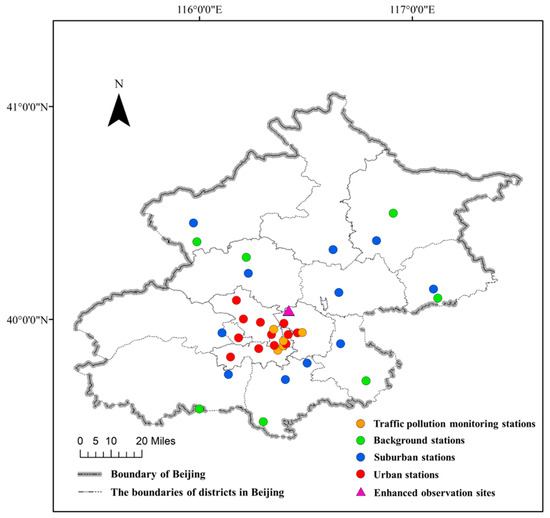
Figure 1.
Distribution map of the 35 ambient air quality monitoring stations in Beijing.
2.1.2. Enhanced Field Observation
The enhanced field observation site (Figure 1) was located on the roof of the Atmospheric Photochemical Smog Chamber Simulation Laboratory of the Chinese Research Academy of Environmental Sciences, Chaoyang District, Beijing (40.04 N, 116.42 E), about 8 m above the ground. The observation site was adjacent to major roads and subway stations, with large residential areas, offices, schools, hospitals, and shopping centers in close proximity, making the area highly trafficked and densely populated. The observation periods were in summer (4 July to 6 August 2019) and autumn (19 September to 11 October 2019). The online observations include conventional pollutants. Two PM2.5 pollution processes were selected for offline sampling during the field observation period, with one in the daytime (07:30–19:00) and one at night (19:30–07:00). The water-soluble inorganic ion components in PM2.5 were also analyzed.
2.2. Observation Items and Analysis Methods
2.2.1. Data on Conventional Pollutants
The gaseous pollutants, SO2, NO2, CO, and O3, were monitored using an SO2 analyzer, model 43i, a NOx analyzer, model 42i, a CO analyzer, model 48i, and an O3 analyzer model 49i (Thermo Scientific, Waltham, MA, USA), respectively. PM10 and PM2.5 were monitored using a 5030 monitor (Thermo Scientific, Waltham, MA, USA). The sampling port of the monitor was equipped with cutting heads, corresponding to the collection of atmospheric particles in different particle size ranges for PM10 and PM2.5 sampling.
2.2.2. PM2.5 Sampling and Inorganic Ion Component Analysis
PM2.5 inorganic ion components were collected in the daytime (07:30–19:00) and nighttime (19:30–07:00) using an off-line sampling method, then the water-soluble inorganic ion components in PM2.5 were analyzed. Since we replaced the filter manually, we needed to replace the filter and clean the sampler before the next sampling was conducted every day, creating a 30-min gap. The PM2.5 samples were collected using quartz filter membranes (Whatman, 203 mm × 254 mm) with a high flow sampler (Thermo Scientific, Waltham, MA, USA). The mass concentration of PM2.5 was analyzed using the gravimetric method. Quartz filter membranes were weighed with an analytical balance (CPA225D, 0.01 mg). The collected PM2.5 filter membrane samples were analyzed using ICS-1000 and ICS-1100 ion chromatographs for water-soluble cations (Ca2+, NH4+, Mg2+, Na+, and K+) and anions (SO42−, NO3−, Cl−, and F−), respectively.
2.3. Quality Control
2.3.1. Online Monitoring of Conventional Pollutants
The ambient air automatic continuous monitoring system included a model 49i (O3), model 48i (CO), model 43i (SO2), model 42i (NO2), and model 5030 SHARP monitor (for PM10 and PM2.5) (Thermo Scientific, Waltham, MA, USA). Data quality assurance and quality control (QA/QC) followed the regulations for automated methods for ambient air quality monitoring (HJ/T 193–2005) [14]. The model 42i, model 48i, and model 43i instruments were calibrated regularly using NO (2 μmol/mol), CO (4.24 μmol/mol), and SO2 (54 μmol/mol) standard gases. NO standard gas is produced by Air Products and Chemicals, Inc. Nitrogen was used as the balance gas. The CO and SO2 standard gases were produced by the Institute for Environmental Reference Materials (IERM) of the China Ministry of Environmental Protection. The model 49i instrument was calibrated annually using the standard reference photometer (SRP) calibration from the IERM. The paper tapes of the PM10 and PM2.5 particulate matter monitor (model 5030 SHARP monitor) were checked and the filter membranes were changed once a week. The cutting heads were cleaned once a week, which meets the requirements of the “Specifications and test procedures for ambient air quality continuous automated monitoring system for PM10 and PM2.5 (HJ 653—2021) [15]”. Leakage detection and flow correction were carried out once a week on the monitor.
2.3.2. Offline Sampling of PM2.5 and Ion Component Analysis
Before PM2.5 sampling, the key components of the high-flow sampler were cleaned with anhydrous ethanol; then, a layer of petroleum jelly was evenly applied to the upper surface of the impact plate, and the flow rate of the sampling system was tested and calibrated. During sampling, tweezers cleaned with anhydrous ethanol were used to replace the filters, and nitrile gloves were worn. After the sampling, the filters were wrapped with clean aluminum foil and stored in the refrigerator. The ICS-1000 and ICS-1100 ion chromatographs were verified and calibrated to ensure that the analysis requirements were met during the ion component analysis of PM2.5. The correlation coefficients of the correction curves were above 0.995. While analyzing the samples, the standard solutions of the midpoint concentration of calibration curves were randomly tested, and the relative errors were controlled within the range of ±10%.
2.4. Data Analysis and Processing
Based on the data from the national urban sites that were monitored (excluding background sites), the over-standard conditions of PM10, PM2.5, and O3 in Beijing from 2016 to 2019 were determined, according to the relevant requirements for the Ambient Air Quality Standards (GB 3095–2012) and Technical Regulation for Ambient Air Quality Assessment (On Trial) (HJ 663–2013) [16,17]. According to the revision notice of Ambient Air Quality Standards (GB 3095–2012) issued by the Ministry of Ecology and Environment in 2018, the data on conventional pollutants used in this study from 2016 to 2019 were recorded under conditions for monitoring data using the reference state (25 °C, 101.325 kPa), while the data of PM2.5 and PM10 were recorded when monitoring in the actual state.
2.4.1. Correlation Analysis
The hourly average mass concentrations of PM10, PM2.5, and SNA were converted into the daily average, seasonal average, and annual average using Microsoft Excel 2020 software (Microsoft, Redmond, WA, USA). The hourly average mass concentration of O3 was converted into the maximum daily 8-h moving average (MDA8 O3) and the annual evaluation value (90th percentile of the maximum daily 8-h moving average). The Pearson correlation coefficient (r) was calculated using SPSS 22 software (International Business Machines Corporation, Armonk, NY, USA) to quantify the correlation among PM2.5, SNA, O3, and OX.
2.4.2. Estimation of Secondary Particle Generation
In this study, the primary and secondary component concentrations in PM2.5 were analyzed using an empirical formula method. The specific method takes carbon monoxide as a tracer of the primary components, and MDA8 O3 represents the degree of photochemical reaction activity [6,18]; the formula expressions are as follows:
where E, G, L, and M represent different O3 concentration ranges (E: MDA8 O3 ≤ 100 μg/m3; G: 100 μg/m3 < MDA8 O3 ≤ 160 μg/m3; L: 160 μg/m3 < MDA8 O3 ≤ 200 μg/m3; M: MDA8 O3 > 200 μg/m3); p: primary pollutant; h: any hour of the day. PM2.5 and CO denote the hourly concentrations of PM2.5 and CO, respectively.
(PM2.5)p,G,h = COG,h × (PM2.5/CO)p,E,h
(PM2.5)p,L,h = COL,h × (PM2.5/CO)p,E,h
(PM2.5)p,M,h = COM,h × (PM2.5/CO)p,E,h
The concentrations of the secondary components of PM2.5 are the observed concentration of PM2.5 minus the concentrations of the primary components of PM2.5 obtained from Formulas (1)–(3). Therefore, the formulas for calculating the concentrations of the secondary components of PM2.5 are:
where (PM2.5)sec,G,h, (PM2.5)sec,L,h, and (PM2.5)sec,M,h represent the concentrations of secondary components in PM2.5 at different O3 pollution levels.
(PM2.5)sec,G,h = (PM2.5)obs,G,h-(PM2.5)p,G,h
(PM2.5)sec,L,h = (PM2.5)obs,L,h-(PM2.5)p,L,h
(PM2.5)sec,M,h = (PM2.5)obs,M,h-(PM2.5)p,M,h
In order to understand the impact of AOC and photochemical reaction activity on secondary particle generation, O3 concentration is usually used as an indicator to reflect the photochemical reaction activity. In order to distinguish the impact of different photochemical reaction activity levels on the generation of secondary particles, the photochemical reaction activity levels were divided into four categories according to O3 concentrations, based on values given in the literature [6,18]:
- (1)
- R0: MDA8 O3 ≤ 100 μg/m3;
- (2)
- R1: 100 < MDA8 O3 ≤ 160 μg/m3;
- (3)
- R2: 160 < MDA8 O3 ≤ 200 μg/m3;
- (4)
- R3: MDA8 O3 > 200 μg/m3.
2.4.3. Calculation of Sulfur Oxidation Rate, Nitrogen Oxidation Rate, and Atmospheric Oxidant (OX) Concentrations
SOR and NOR are often used to measure the secondary conversion efficiency of gaseous precursors such as SO2 and NOx. The higher the values of SOR and NOR, the higher the secondary transformation degree of SO2 and NO2 in the atmosphere. The formulas are as follows:
where N1 and N2 represent the concentrations of NO3− and NO2 in mol/m3, respectively; S1 and S2 represent the concentrations of SO42− and SO2 in mol/m3, respectively.
SOR = N1/(N1 + N2)
NOR = S1/(S1 + S2)
OX is commonly used to indicate AOC. In this study, OX concentrations from 2016 to 2019 at four types of monitoring stations were calculated to characterize the AOC at different periods. The calculation method is as follows:
where ρ(OX), ρ(O3), and ρ(NO2) represent the concentrations of OX, O3, and NO2 in μg/m3, respectively.
ρ(OX) = ρ(O3) + ρ(NO2)
3. Results and Discussion
3.1. Changes in OX Concentration and Its Correlation with PM2.5 Concentration
3.1.1. Interannual Change and Seasonal Change of OX Concentration
As seen in the variations in the monthly average concentrations of OX in Beijing from 2016 to 2019, the OX concentrations reached their highest levels in June (142–154 μg/m3) and the lowest in October–December (67–80 μg/m3), in these four years. This showed that the AOC was usually the highest in summer and the lowest in winter (Figure 2).
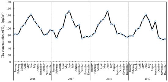
Figure 2.
Inter-month variations in atmospheric oxidant capacity (OX) in Beijing from 2016 to 2019.
High OX concentrations have long been considered an important feature of air pollution in Beijing [11,19,20]. As shown in Figure 3, the annual mean OX concentrations at urban stations, suburban stations, traffic pollution monitoring stations, and background stations in Beijing from 2016 to 2019 were 92–107 μg/m3, 90–105 μg/m3, 96–114 μg/m3, and 84–98 μg/m3, respectively. The annual mean OX concentrations of the four types of stations fluctuated little from 2016 to 2018, but the annual mean OX concentration in 2019 showed a significant decline. Compared to those in 2018, the annual mean values at urban stations, suburban stations, traffic pollution monitoring stations, and background stations decreased by 11, 11, 12, and 13 μg/m3, respectively. The annual OX values of the four types of stations, listed in descending order, were traffic pollution monitoring stations, urban stations, suburban stations, and background stations. Although the O3 concentration at the traffic pollution monitoring stations was significantly lower than that of the other three types of monitoring stations, the OX concentration for the traffic pollution monitoring stations was higher than those of the other three types of monitoring stations, due to their high NO2 concentration.
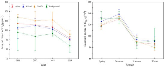
Figure 3.
Inter-annual and seasonal changes of atmospheric oxidant capacity (OX) in Beijing from 2016 to 2019.
From 2016 to 2019, the AOC of the four seasons in descending order were summer, spring, autumn, and winter, and the OX concentrations in spring, summer, autumn, and winter were 130, 119, 88, and 86 μg/m3 at urban stations, 129, 116, 84, and 81 μg/m3 at suburban stations, 137, 123, 98, and 88 μg/m3 at traffic pollution monitoring stations, and 114, 113, 75, and 79 μg/m3 at background stations, respectively. As shown in Table 1, the O3/OX ratio was 0.74 in summer, which was significantly higher than the annual mean value. The correlation coefficient between O3 and OX was up to 0.96, indicating that the AOC was mainly affected by O3 concentration in summer, which could significantly increase the level of OX concentration in summer. The OX concentration was lowest in winter, which indicated that the AOC was low in winter. The NO2/OX ratio was higher (0.36) than that in winter, and the correlation coefficient of NO2 and OX was up to 0.81, indicating that the change in OX concentration in winter was mainly caused by the change in NO2 concentration; NO2 had a more important effect on the AOC value in winter.

Table 1.
Ratio and correlation coefficients of NO2 and O3 to OX over four seasons.
3.1.2. Correlation between OX and PM2.5 Concentrations
In order to explore the distribution relationship between OX and PM2.5 concentrations, different colors were used in Figure 4 to show the distribution characteristics of OX and PM2.5 mass concentrations for four seasons. As shown in Figure 4, PM2.5 and OX were positively correlated in all four seasons, and PM2.5 concentration increased with the increase in OX concentration, especially in winter, when the slope of PM2.5 and OX was 0.18, indicating that the increase in PM2.5 concentration in winter was more sensitive to changes in OX concentration. This was mainly due to the higher NO2/OX ratio in winter, while the increase in PM2.5 was mainly affected by the change in NO2 concentration. Conversely, the slope of PM2.5 and OX in summer was 0.8, indicating that the increase in PM2.5 in summer was less sensitive to changes in OX concentration. However, due to the large fluctuation of OX concentration in summer, when the OX concentration was significantly higher than that in other seasons, the stronger AOC in summer also made a great contribution to the increase in PM2.5.
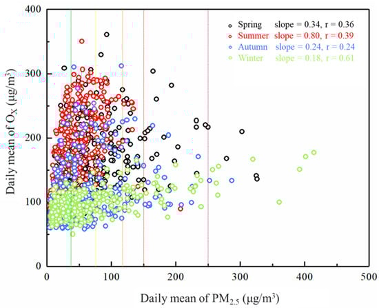
Figure 4.
Mass concentration distribution characteristics of PM2.5 and atmospheric oxidant capacity (OX) in Beijing from 2016 to 2019. The vertical dashed lines in the figure represent different pollution levels: green—excellent; yellow—good; orange—light contamination; red—moderate pollution; purple—heavy pollution.
PM2.5 showed a good correlation with OX in winter with a correlation coefficient of 0.61, followed, in summer, by a correlation coefficient of 0.39. The correlation coefficient between PM2.5 and OX in spring was 0.36. The lowest correlation coefficient was 0.24 in autumn. PM2.5 showed a positive correlation with OX in the four seasons, especially in summer and winter, indicating that the enhancement of AOC could promote an increase in PM2.5 concentration, to a certain extent.
3.2. Evaluation of the Effect of Atmospheric Photochemical Reaction Activity on Atmospheric Secondary Particle Generation
3.2.1. Classification of Photochemical Reaction Activity
Figure 5 shows the correlation between CO and the daily mean mass concentration of PM10 and PM2.5 at different photochemical reaction activity levels. When MDA8 O3 ≤ 100 μg/m3, there was a good linear relationship between CO and PM2.5 and PM10; the correlation coefficients were 0.88 and 0.72, respectively. However, when MDA8 O3 was 100–160 μg/m3, 160–200 μg/m3, and greater than 200 μg/m3, the correlation between CO and PM10 and PM2.5 decreased, especially the correlation between CO and PM10, which decreased significantly to 0.45, 0.41, and 0.39, respectively, along with the increase in O3 concentration. This indicated that when the MDA8 O3 value was less than 100 μg/m3, the photochemical reaction activity was less marked, and the observed particle concentration was mainly contributed by the particles from the primary emission. This only contained a few particles from the secondary generation, resulting in a significant correlation between CO, PM10, and PM2.5. The increase in MDA8 O3 concentration also indicated that the photochemical reaction activity increased, which led to the generation of more secondary particles and further promoted the increase in PM10 and PM2.5 concentrations, resulting in the deterioration of the correlation between CO and PM10 and PM2.5. In addition, when MDA8 O3 ≤ 100 μg/m3, the intercept of the regression line was low, indicating that CO and PM2.5 had a certain homology, and the levels drawn from other sources were relatively low. In summary, when the photochemical reaction activity was low, CO showed a good correlation with PM10 and PM2.5, respectively. In this study, the linear fitting of PM2.5 and CO was better than that of PM10 and CO, and the ratio of PM2.5/PM10 from 2016 to 2019 was 72.05%, 62.18%, 61.5%, and 59.36%, respectively. Therefore, when evaluating the influence of the photochemical reaction activity on the generation of secondary particles, the ratio of PM2.5/CO was more suitable for estimating the generation of secondary particles than PM10/CO. The PM2.5/CO ratio was selected as the tracer and used to evaluate secondary particle generation.
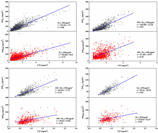
Figure 5.
Linear fitting between the daily mean of PM10, PM2.5, and CO for different photochemical activities in Beijing from 2016 to 2019.
3.2.2. Effect of Different Photochemical Reaction Activities on the Generation of Atmospheric Secondary Particles
Based on the classification of photochemical reaction activity, the diurnal concentration variation curves of primary PM2.5 emissions under different O3 concentration ranges were calculated. In Figure 6, the values R1: 100 < MDA8 O3 ≤ 160 μg/m3, R2: 160 < MDA8 O3 ≤ 200 μg/m3, and R3: MDA8 O3 > 200 μg/m3 correspond to the PM2.5 mass concentration from primary emissions, at (PM2.5)p,G,h, (PM2.5)p,L,h, and (PM2.5)p,M and H,h, respectively. As shown in Figure 6, the curves of the primary PM2.5 emission concentrations corresponding to the three photochemical reaction activities had a similar trend, which rose rapidly after 05:00 and continued to peak at around 09:00, mainly because Beijing had a “morning peak” period between 06:00 and 09:00. The large volume of traffic flow led to a rapid increase in PM2.5 emission concentration. After 09:00, primary PM2.5 emissions began to decline gradually and then began to rise again around 17:00, during the “evening peak”. The primary PM2.5 emission concentration increased with photochemical reaction activity, indicating that the primary PM2.5 emission was overestimated when the photochemical reaction activity was strong. Therefore, the difference between the diurnal concentration variation curves of the primary PM2.5 emission, when the photochemical reaction activity was R1, R2, and R3, and the curve when the photochemical reaction activity was R0 are a result of the overestimation of primary PM2.5 emission, when the photochemical reaction activity was R1, R2, and R3, respectively. These differences were added to the calculation of secondary PM2.5 generation concentrations to reduce errors in the estimation of secondary PM2.5 generation.
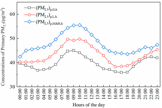
Figure 6.
Estimation of the daily variation of primary PM2.5 emissions under different photochemical reaction activity conditions in Beijing, from 2016 to 2019.
Figure 7 shows the diurnal variation of the estimated mass concentration of secondary PM2.5 generation under different photochemical reaction activity levels in Beijing from 2016 to 2019. As shown in Figure 7, the diurnal variation trends of the mass concentration of secondary PM2.5 generation, corresponding to the three types of photochemical reaction activities R1, R2, and R3, were quite different. When the photochemical reaction activity was R1, 100 < MDA8 O3 ≤ 160 μg/m3, the secondary PM2.5 generation peaked at 15.14 μg/m3 at 04:00 and reached its minimum of 11.1 μg/m3 at 07:00. Then, it gradually rose until 17:00, when it reached its maximum of 17.72 μg/m3. Subsequently, it decreased slightly. When the photochemical reaction activity was R2, 160 < MDA8 O3 ≤ 200 μg/m3, the secondary PM2.5 generation peaked at 23.33 μg/m3 at 05:00 and reached a trough value of 19.88 μg/m3 at 07:00. Then, it began to rise rapidly, reached its maximum of 28.66 μg/m3 at 11:00, and then began to decline gradually. It continued to decline until 21:00 and reached its minimum of 14.77 μg/m3. When the photochemical reaction activity was R3, MDA8 O3 > 200 μg/m3, secondary PM2.5 generation began to rise from 00:00 until 03:00–07:00 and then remained stable at about 27 μg/m3. After 08:00, it began to rise rapidly and reached the maximum of 36.33 μg/m3 at 11:00. Then, it gradually decreased and continued to reach the minimum of 16 μg/m3 at 21:00. In conclusion, the stronger the photochemical reaction activity, the greater the secondary PM2.5 generation. Secondary PM2.5 generation increased rapidly with the increase in photochemical reaction activity in the daytime and reached the maximum value at 17:00, 11:00, and 11:00, respectively, under different photochemical reaction activity levels of R1, R2, and R3. In addition, the secondary PM2.5 generation at night was much lower than that in the daytime, indicating that the strong photochemical reaction activity and AOC in the daytime were more conducive to the generation of secondary particles.
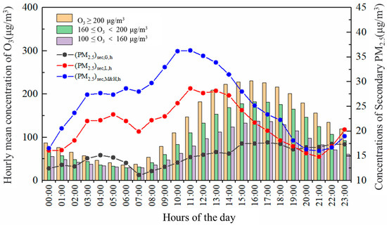
Figure 7.
Estimation of the daily variations in secondary generation PM2.5 under different photochemical reaction activity conditions in Beijing from 2016 to 2019.
Figure 8 shows the mass concentrations and proportions of PM2.5 from primary emission and secondary generation at different photochemical reaction activity levels during the whole study period. Meanwhile, in order to understand the proportion of secondary particles under strong AOC, the estimated values in summer, when the atmospheric oxidation was strongest, are shown separately in Figure 8b. The results showed that from 2016 to 2019, the secondary PM2.5 generation corresponding to the photochemical reaction activities of R1, R2, and R3 accounted for 26%, 35%, and 42% of the total PM2.5 mass concentration, respectively. This indicates that the stronger the atmospheric photochemical reaction activity, the more numerous the secondary particles generated, and the higher the proportion. Strong photochemical reactions in the atmosphere could promote the oxidation process of precursor substances such as SO2, NO2, and VOCs, and further generate SIA and SOA, thus promoting the generation of secondary particles. Especially in summer, the increase in AOC had a more obvious promoting effect on secondary particle generation. Intense solar radiation and higher temperatures in summer increased the AOC; therefore, the increased AOC could promote the formation of secondary particles. In summer, the secondary PM2.5 generation corresponding to the photochemical reaction activities of R1, R2, and R3 accounted for 26%, 39%, and 49%, respectively. Stronger AOC values in summer led to the formation of more secondary particles, which might be the main factor behind the positive correlation between O3 and PM2.5 in summer.
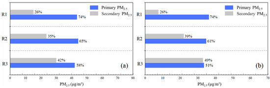
Figure 8.
PM2.5 mass concentration and the percentage of primary emission and secondary generation for different photochemical reaction activities in Beijing: (a) 2016–2019, (b) summer 2016–2019. R1: 100 < MDA8 O3 ≤ 160 μg/m3; R2: 160 < MDA8 O3 ≤ 200 μg/m3; R3: MDA8 O3 > 200μg/m3.
3.3. Effect of AOC on the Formation of Secondary Inorganic Components in Atmospheric Particulate Matter
3.3.1. Composition Characteristics of Water-Soluble Inorganic Ions in PM2.5
From 2016 to 2019, the mass concentrations of water-soluble inorganic ions in PM2.5 at the enhanced observation site were as follows, from high to low: NO3−, SO42−, NH4+, Na+, Ca2+, Cl−, K+, Mg2+, and F−. The most important anion component was NO3−, accounting for 40.69% of the total ions, followed by SO42− (21.95%), Cl− (3.37%), and F− (0.37%). NH4+ was the most important cationic component, accounting for 14.46% of the total ions, followed by Na+ (9.53%), Ca2+ (6.66%), K+ (2.11%), and Mg2+ (0.86%). SNA were the most important secondary water-soluble inorganic ions in PM2.5 and accounted for 50.7–94.4% of the total mass concentration of water-soluble inorganic ions, indicating that SIA represent important components of PM2.5.
The composition characteristics of PM2.5 inorganic ions were different between the daytime and nighttime. The composition characteristics of water-soluble inorganic ions of PM2.5 in the daytime and nighttime are shown in Figure 9. The concentration of water-soluble inorganic ions in PM2.5 in the daytime was significantly higher than that at night, and the sums of mass concentrations of water-soluble inorganic ions in PM2.5 in the daytime and nighttime were 34.85 μg/m3 and 30.36 μg/m3, respectively. The concentrations of 9 kinds of water-soluble ions in PM2.5 in the daytime were all higher than those at night, especially the mass concentrations of SNA. This indicates that, compared with the levels at night, the generation of SNA in PM2.5 was higher in the daytime, with higher photochemical reaction activity and AOC levels.
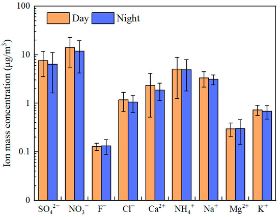
Figure 9.
Daytime and nighttime PM2.5 water-soluble inorganic ion composition characteristics.
3.3.2. Sulfur and Nitrogen Conversion Rates of SO2 and NO2 in the Atmosphere
The oxidation pathways of SO2 and NO2 in the atmosphere are mainly a gaseous oxidation reaction and heterogeneous oxidation reaction. These two pathways are affected by atmospheric oxidants, such as OH, O3, H2O2, and NO3. Therefore, an increase in AOC can promote the oxidation reaction between SO2 and NO2, resulting in an increase in SOR and NOR values. Figure 10 shows the SOR and NOR distribution characteristics in the daytime and at nighttime during the observation period. The values for SOR (0.61) and NOR (0.26) in the daytime were higher than for SOR (0.55) and NOR (0.16) at nighttime, indicating that the conversion rates of SO2 and NO2 to SO42− and NO3− were higher than those at nighttime. This was because the AOC was enhanced by active photochemical reactivity in the daytime; thus, the oxidation reaction of SO2 and NO2 was promoted. Compared with other domestic cities, the SOR value of Beijing from July to September was higher than that of Shanghai, Xi’an, and Taiyuan; the NOR value was higher than that of Shanghai and Taiyuan, but lower than that of Jiaozuo, Puyang, and Xi’an (Table 2).
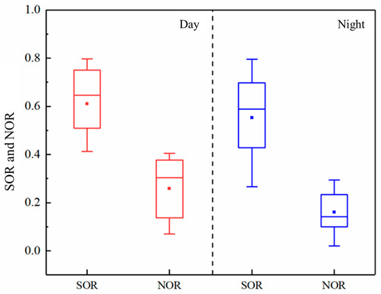
Figure 10.
Daytime and nighttime SOR and NOR distribution characteristics.
Table 2.
Comparison of SOR and NOR values reported in the literature during the observation period.
3.3.3. Correlation between OX and Secondary Inorganic Salts, SOR, and NOR in PM2.5
SO42− and NO3− are mainly generated through the secondary reaction of the gaseous pollutants SO2 and NO2, while the oxidation efficiency of SO2 and NO2 is related to the AOC [26,27]. The correlation coefficients of PM2.5, OX, SOR, NOR, and SNA were calculated, as shown in Table 3. PM2.5 was positively correlated with OX, SOR, NOR, and SNA. OX was positively correlated with SOR and NOR, with correlation coefficients of 0.25 and 0.36, respectively (Figure 11). OX was positively correlated with SO42−, NO3−, and NH4+, and the correlation coefficients were 0.35, 0.41, and 0.32, respectively, indicating that strong AOC could improve the conversion rates of SO2 and NO2 and, thus, promote the generation of SNA.
Table 3.
Correlation coefficients between OX, SOR, NOR, and SNA.
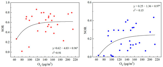
Figure 11.
Exponential fitting of OX concentration to SOR and NOR during the observation period.
The coefficient of determination (R2) between SOR and OX reached 0.91, while that between NOR and OX was only 0.15. This may be due to the fact that nitrate generation during the observation period may not only have been affected by AOC but may also have been greatly affected by environmental factors, such as temperature and humidity. In contrast, environmental factors have little influence on sulfate production [4,28]. Due to the simultaneous increase in atmospheric oxidizing capacity, changes in precursor concentration, air temperature, relative humidity, and other conditions may have a certain impact on the generation of sulfate and nitrate. Therefore, the relationship between OX and SOR, and the relationship between OX and NOR, were both nonlinear. This study exponentiated the sulfate conversion rate and nitrate conversion rate against the change in OX concentration. The results showed that when the OX concentration was less than around 140 μg/m3, SOR and NOR significantly increased with the increase in OX concentration, indicating that the atmospheric oxidizing capacity had a significant promoting effect on SOR and NOR. However, when the OX concentration was higher than around 140 μg/m3, the magnitude of the increase in SOR and NOR was smaller, indicating that atmospheric oxidizing capacity may no longer be the determining factor for sulfate and nitrate generation. At this time, the generation of sulfate and nitrate may be influenced by other factors, such as precursor concentration, temperature, and relative humidity [29].
4. Conclusions
From 2016 to 2019, the annual OX values in Beijing, listed in descending order, were traffic pollution monitoring stations, urban stations, suburban stations, and background stations. In 2019, the annual mean of OX at all stations in Beijing showed a significant decline. Compared to those in 2018, the AOC values at urban stations, suburban stations, traffic pollution monitoring stations, and background stations decreased by 11, 11, 12, and 13 μg/m3, respectively. The AOC of the four seasons, in descending order, were summer, spring, autumn, and winter. The concentration of OX was mainly affected by the concentration of O3 in summer, while the concentration of NO2 had the most important effect on OX in winter.
The results of the PM2.5 secondary generation evaluation showed that from 2016 to 2019, the secondary PM2.5 generation corresponding to the photochemical reaction activities of R1, R2, and R3 accounted for 26%, 35%, and 42% of the total PM2.5 mass concentration, respectively. It is indicated that the stronger atmospheric photochemical reaction activity promoted the generation of secondary particles, resulting in their higher proportion in PM2.5.
Secondary PM2.5 generation increased rapidly with the increase in photochemical reaction activity in the daytime and reached the maximum values at 17:00, 11:00, and 11:00, respectively, under the different photochemical reaction activity levels of R1, R2, and R3. SNA, SOR, and NOR values in the daytime were higher than those at nighttime, indicating that the daytime, with its higher photochemical activity and greater AOC, was more conducive to SNA generation. OX showed a positive correlation with SNA, SOR, and NOR, indicating that the generation of SNA in PM2.5 was promoted when the concentration of OX was high, thereby leading to an increase in PM2.5 concentration. When the OX concentration was less than around 140 μg/m3, SOR and NOR significantly increased with an increase in OX concentration. However, when the OX concentration was higher than around 140 μg/m3, the magnitude of the increase in SOR and NOR was smaller, indicating the relationship between OX and SOR, and the relationship between OX and NOR, were both nonlinear.
When establishing emission reduction measures for precursors, it is necessary to comprehensively consider the impact of increasing AOC on the generation of secondary components in PM2.5, so as to further reduce the emission of highly reactive precursors and reduce AOC. The decline in AOC will help achieve PM2.5 control targets in China in the future.
Author Contributions
Conceptualization, W.C., L.L. and H.L.; data curation, W.C., L.L., Y.Z., X.Y. and Y.J.; formal analysis, W.C. and L.L.; funding acquisition, H.L.; investigation, W.C.; methodology, W.C., L.L. and H.L.; project administration, H.L. and F.C.; resources, Y.Z., Y.C., G.Z., X.Y. and Y.J.; supervision, H.L.; validation, W.C., L.L. and H.L.; visualization, W.C. and L.L.; writing—original draft, W.C. and L.L.; writing—review and editing, H.L. All authors have read and agreed to the published version of the manuscript.
Funding
This work was financially supported by programs from the Beijing Municipal Science & Technology Commission (No. Z181100005418015), the National Research Program for Key Issues in Air Pollution Control (DQGG202121). the National Key Research and Development Program of China (No. 2019YFC0214501).
Institutional Review Board Statement
Not applicable.
Informed Consent Statement
Not applicable.
Data Availability Statement
The observation and modeling data are available from the corresponding author upon reasonable request.
Acknowledgments
The authors acknowledge all funders.
Conflicts of Interest
The authors declare no conflict of interest.
References
- Beijing Municipal Ecology and Environment Bureau. Beijing Ecology and Environment Statement 2019; Beijing Municipal Ecology and Environment Bureau: Beijing, China, 2019.
- Beijing Municipal Ecology and Environment Bureau. Beijing Ecology and Environment Statement 2016; Beijing Municipal Ecology and Environment Bureau: Beijing, China, 2016.
- Zang, H.; Zhao, Y.; Huo, J.; Zhao, Q.; Fu, Q.; Duan, Y.; Shao, J.; Huang, C.; An, J.; Xue, L.; et al. High atmospheric oxidation capacity drives wintertime nitrate pollution in the eastern Yangtze River Delta of China. Atmos. Chem. Phys. 2022, 22, 4355–4374. [Google Scholar] [CrossRef]
- Tan, Z.; Wang, H.; Lu, K.; Dong, H.; Liu, Y.; Zeng, L.; Hu, M.; Zhang, Y. An Observational Based Modeling of the Surface Layer Particulate Nitrate in the North China Plain during Summertime. JGR Atomspheres 2021, 126, e2021JD035623. [Google Scholar] [CrossRef]
- Liu, P.; Ye, C.; Xue, C.; Zhang, C.; Mu, Y.; Sun, X. Formation mechanisms of atmospheric nitrate and sulfate during the winter haze pollution periods in Beijing: Gas-phase, heterogeneous and aqueous-phase chemistry. Atmos. Chem. Phys. 2020, 20, 4153–4165. [Google Scholar] [CrossRef]
- Jia, M.; Zhao, T.; Cheng, X.; Gong, S.; Zhang, X.; Tang, L.; Liu, D.; Wu, X.; Wang, L.; Chen, Y. Inverse Relations of PM2.5 and O3 in Air Compound Pollution between Cold and Hot Seasons over an Urban Area of East China. Atmosphere 2017, 8, 59. [Google Scholar] [CrossRef]
- Zhu, J.; Chen, L.; Liao, H.; Dang, R. Correlations between PM2.5 and Ozone over China and Associated Underlying Reasons. Atmosphere 2019, 10, 352. [Google Scholar] [CrossRef]
- Wang, P.; Zhu, S.; Zhang, M.; Shao, T. Atmospheric oxidation capacity and its contribution tosecondary pollutants formation. Chin. Sci. Bull. 2022, 67, 2069–2078. [Google Scholar] [CrossRef]
- Wen, L.; Xue, L.; Wang, X.; Xu, C.; Chen, T.; Yang, L.; Wang, T.; Zhang, Q.; Wang, W. Summertime fine particulate nitrate pollution in the North China Plain: Increasing trends, formation mechanisms and implications for control policy. Atmos. Chem. Phys. 2018, 18, 11261–11275. [Google Scholar] [CrossRef]
- Kim, J.Y.; Song, C.H.; Ghim, Y.S.; Won, J.G.; Yoon, S.C.; Carmichael, G.R.; Woo, J.H. An investigation on NH3 emissions and particulate NH4+–NO3− formation in East Asia. Atmos. Environ. 2006, 40, 2139–2150. [Google Scholar] [CrossRef]
- Feng, T.; Zhao, S.; Bei, N.; Liu, S.; Li, G. Increasing atmospheric oxidizing capacity weakens emission mitigation effort in Beijing during autumn haze events. Chemosphere 2021, 281, 130855. [Google Scholar] [CrossRef]
- Xie, X.; Hu, J.; Qin, M.; Guo, S.; Hu, M.; Wang, H.; Lou, S.; Li, J.; Sun, J.; Li, X.; et al. Modeling particulate nitrate in China: Current findings and future directions. Environ. Int. 2022, 166, 107369. [Google Scholar] [CrossRef]
- Peng, J.; Hu, M.; Shang, D.; Wu, Z.; Du, Z.; Tan, T.; Wang, Y.; Zhang, F.; Zhang, R. Explosive Secondary Aerosol Formation during Severe Haze in the North China Plain. Environ. Sci. Technol. 2021, 55, 2189–2207. [Google Scholar] [CrossRef]
- Ministry of Ecology and Environment of the People’s Republic of China. Automated Methods for Ambient Air Quality Monitoring; Ministry of Ecology and Environment of the People’s Republic of China: Beijing, China, 2005.
- Ministry of Ecology and Environment of the People’s Republic of China. Specifications and Test Procedures for Ambient Air Quality Continuous Automated Monitoring System for PM10 and PM2.5 (HJ 653–2021); Ministry of Ecology and Environment of the People’s Republic of China: Beijing, China, 2021.
- Ministry of Ecology and Environment of the People’s Republic of China. Ambient Air Quality Standards (GB 3095-2012); Ministry of Ecology and Environment of the People’s Republic of China: Beijing, China, 2012.
- Ministry of Ecology and Environment of the People’s Republic of China. Technical Regulation for Ambient Air Quality Assessment (On Trial) (HJ 663-2013); Ministry of Ecology and Environment of the People’s Republic of China: Beijing, China, 2013.
- Chang, S.-C.; Lee, C.-T. Secondary aerosol formation through photochemical reactions estimated by using air quality monitoring data in Taipei City from 1994 to 2003. Atmos. Environ. 2007, 41, 4002–4017. [Google Scholar] [CrossRef]
- Wei, W.; Wang, Y.; Bai, H.; Wang, X.; Cheng, S.; Wang, L. Insights into atmospheric oxidation capacity and its impact on PM2.5 in megacity Beijing via volatile organic compounds measurements. Atmos. Res. 2021, 258, 105632. [Google Scholar] [CrossRef]
- Lu, K.; Fuchs, H.; Hofzumahaus, A.; Tan, Z.; Wang, H.; Zhang, L.; Schmitt, S.H.; Rohrer, F.; Bohn, B.; Broch, S.; et al. Fast Photochemistry in Wintertime Haze: Consequences for Pollution Mitigation Strategies. Environ. Sci. Technol. 2019, 53, 10676–10684. [Google Scholar] [CrossRef]
- Wang, L.; Wang, X.; Wang, M.; Yu, G. Spatial and Temporal Distribution and Potential Source of Atmospheric Pollution in Jiaozuo City. Res. Environ. Sci. 2020, 33, 820–830. [Google Scholar] [CrossRef]
- Chen, C.; Wang, T.; Li, Y.; Ma, H.; Chen, P.; Wang, D.; Zhang, Y.; Qiao, Q.; Li, G.; Wang, W. Pollution Characteristics and Source Apportionment of Fine Particulate Matter in Autumn and Winter in Puyang, China. Environ. Sci. 2019, 40, 3421–3430. [Google Scholar] [CrossRef]
- Zhou, M.; Chen, C.; Wang, H.; Huang, C.; Su, L.; Chen, Y.; Li, L.; Qiao, Y.; Chen, M.; Huang, H.; et al. Chemical characteristics of particulate matters during air pollution episodes in autumn of Shanghai, China. Acta Sci. Circumstantiae 2012, 32, 81–92. [Google Scholar] [CrossRef]
- Shen, Z.; Huo, Z.; Han, Y.; Cao, J.; Zhao, J.; Zhang, T. Chemical Composition of Water-Soluble Ions in Aerosols over Xi’an in Heating and Non-Heating Seasons. Plateau Meteorol. 2009, 28, 151–158. [Google Scholar]
- Guo, W.; Wang, K.; Guo, X.; Yan, Y. Characteristics of sulfur and nitrogen conversion in the aerosol, Taiyuan. Environ. Chem. 2016, 35, 11–17. [Google Scholar] [CrossRef]
- Wang, Z.; Li, Y.; Chen, T.; Zhang, D.; Sun, F.; Wang, X.; Huan, N.; Pan, L. Analysis on diurnal variation characteristics of ozone and correlations with its precursors in urban atmosphere of Beijing. China Environ. Sci. 2014, 34, 3001–3008. [Google Scholar]
- Huang, X.-F.; Cao, L.-M.; Tian, X.-D.; Zhu, Q.; Saikawa, E.; Lin, L.-L.; Cheng, Y.; He, L.-Y.; Hu, M.; Zhang, Y.-H.; et al. Critical Role of Simultaneous Reduction of Atmospheric Odd Oxygen for Winter Haze Mitigation. Environ. Sci. Technol. 2021, 55, 11557–11567. [Google Scholar] [CrossRef]
- Xue, J.; Yuan, Z.; Griffith, S.M.; Yu, X.; Lau, A.K.H.; Yu, J.Z. Sulfate Formation Enhanced by a Cocktail of High NOx, SO2, Particulate Matter, and Droplet pH during Haze-Fog Events in Megacities in China: An Observation-Based Modeling Investigation. Environ. Sci. Technol. 2016, 50, 7325–7334. [Google Scholar] [CrossRef]
- Li, K.; Jacob, D.J.; Liao, H.; Zhu, J.; Shah, V.; Shen, L.; Bates, K.H.; Zhang, Q.; Zhai, S. A two-pollutant strategy for improving ozone and particulate air quality in China. Nat. Geosci. 2019, 12, 906–910. [Google Scholar] [CrossRef]


Disclaimer/Publisher’s Note: The statements, opinions and data contained in all publications are solely those of the individual author(s) and contributor(s) and not of MDPI and/or the editor(s). MDPI and/or the editor(s) disclaim responsibility for any injury to people or property resulting from any ideas, methods, instructions or products referred to in the content. |
© 2023 by the authors. Licensee MDPI, Basel, Switzerland. This article is an open access article distributed under the terms and conditions of the Creative Commons Attribution (CC BY) license (https://creativecommons.org/licenses/by/4.0/).