Article

Optimal Probability Distribution and Applicable Minimum Time-Scale for Daily Standardized Precipitation Index Time Series in South Korea

Division of Earth Environmental System Science, Pukyong National University, Busan 48513, Republic of Korea
*
Author to whom correspondence should be addressed.
Atmosphere 2023, 14(8), 1292; https://doi.org/10.3390/atmos14081292
Submission received: 20 July 2023 / Revised: 5 August 2023 / Accepted: 14 August 2023 / Published: 16 August 2023
(This article belongs to the Section Meteorology)

Abstract

:
The Standardized Precipitation Index (SPI) is a standardized measure of the variability of precipitation and is widely used for drought assessment around the world. In general, the probability distribution used to calculate the SPI in many studies is Gamma. In addition, a monthly time-scale is applied to calculate the SPI to assess drought based on atmospheric moisture supply over the medium-to-long term. However, probability distributions other than Gamma are applied in various regions, and the need for a daily time-scale is emerging as concerns about fresh drought increase. There are two main innovations of our work. The first is that we investigate the optimal probability distribution of daily SPIs rather than monthly SPIs, and the second is that we address the issue of determining the minimum time-scale that can be applied when applying a daily time-scale. In this study, we investigate the optimal probability distribution and the minimum-applicable time-scale for calculating the daily SPI using daily precipitation time series observed over 42 years at 56 sites in South Korea. Six candidate probability distributions (Gumbel, Gamma, GEV, Log-logistic, Log-normal, and Weibull) and ten time-scales (5 day, 10 day, 15 day, 21 day, 30 day, 60 day, 90 day, 180 day, 270 day, and 365 day) were applied to calculate the daily SPI. A chi-square test and AIC were applied to investigate the appropriate probability distribution for each time-scale, and the normality of the daily SPI time series derived from each probability distribution were compared. The Weibull distribution was suitable for calculating the daily SPI for short time-scales of 30 days or less, while the GEV distribution was suitable for longer time-scales of 270 days or more. However, overall, Gamma was found to be the best probability distribution. While there were some regional variations, the minimum time-scales that could be applied per season were as follows: 15 days for spring and summer, 21 days for fall, and 30 days for winter. It is shown that the minimum time-scale depends on how many zero values are included in the moving cumulative-precipitation time series, and it is shown that it is appropriate to have less than about 2.5%. Finally, the applicability of the GEV distribution is investigated.

1. Introduction

Due to its flexibility, spatiotemporal comparability, and simple calculation, the Standardized Precipitation Index (SPI) [1] has been widely applied to drought assessment worldwide [2,3,4,5,6,7,8,9,10]. WMO [11] recommends the use of the SPI for meteorological drought assessment because it allows users to confidently compare past and present droughts between different climates and geographic locations. However, the SPI is a relative measure that depends on the probability distribution function (PDF) adopted [12,13]. The appropriate PDFs for cumulative precipitation at different time-scales and the minimum time-scale for calculating cumulative precipitation need to be further investigated in the context of drought studies applying the SPI at different locations [14,15,16].
As the climate is changing globally, the transition between wet and dry periods is shortening in many regions, and the frequency of flush droughts is increasing. This is also the case in South Korea, where more frequent droughts, more intense droughts, and more rapidly developing droughts are expected to occur [17,18,19]. Therefore, it is necessary to quickly detect changes in wetness and dryness and, for this purpose, it is necessary to analyze droughts on a daily time-scale, which is shorter than the monthly time-scale currently used.
The proper selection of the PDF for precipitation is a prerequisite for a reliable SPI calculation. Different PDFs (even different parameters of the same PDF) will lead to different SPI values [2]. The original formulation of the SPI calculation by McKee et al. [1] assumed that the cumulative precipitation follows a Gamma distribution. The Gamma distribution has been found to be the optimal PDF for SPI calculations in most parts of the world. For example, Stagge et al. [7] recommended the use of the Gamma distribution for general use in calculating the SPI over all regions of Europe and across all time-scales. Okpara et al. [8] showed that the Gamma distribution was the best fit for monthly rainfall in West Africa. Blain et al. [9] recommended the use of the Gamma distribution for calculating SPI on 1- to 12-month time-scales in the tropical–subtropical region of Brazil. Zhao et al. [20] showed that the Gamma distribution exhibited the greatest stability across different time-scales in China. However, a number of studies have shown that other PDFs are more appropriate in other climate regions and at other time-scales. Angelidis et al. [21] showed that the SPI at a 12-month or 24-month time-scale can use a log-normal or normal probability distribution instead of a gamma distribution and produce almost the same results. Sienz et al. [5] found that the Weibull distribution provided a markedly improved fit for the monthly precipitation over Europe and the continental United States compared to the Gamma distribution. Guenang et al. [10] reported that both the Gamma and Weibull distributions were the best fit for SPI calculations at time-scales of 9 months or less over most of Central Africa. Pieper et al. [22] advocated the use of the Weibull distribution as the basis for SPI calculations for land areas around the world. However, most studies have investigated the best PDFs for calculating the SPI on monthly time-scales, and few have investigated the best PDFs for calculating the SPI on sub-monthly time-scales.
The SPI can be calculated at different time-scales. The time-scales used in the literature vary from 1 month to 48 months, and the different time-scales reflect the impact of drought on the availability of different water resources [23,24]. For example, to analyze meteorological droughts, the SPI calculated at a time-scale of 1 month or 2 months is applied, agricultural droughts are analyzed at a time-scale of 3 months to 6 months, and hydrological droughts are analyzed at a time-scale of 6 months up to 24 months [11]. However, caution is needed when analyzing SPIs on sub-monthly time-scales in low-precipitation regions or during periods of low precipitation. Wu et al. [25] found that when calculating the SPI for shorter time-scales, such as 1 week in the eastern United States, it was possible in all seasons. However, they found that in the western United States, the high frequency of precipitation-free days can result in unreliable SPI time series [25]. In fact, the difficulty of estimating the SPI time series for dry regions or dry periods due to statistical problems related to inaccuracies in estimating the parameters of the Gamma distribution has already been recognized in many studies [26]. However, not enough quantitative research has been conducted on the minimum time-scale that can be applied in different climate regions or in different periods of the year. There are some studies that suggest that, on a monthly time-scale, the Weibull distribution is mainly suitable for shorter time-scales and the Gamma distribution is more suitable for longer time-scales [7].
The SPI is one of the main drought indices recommended by the South Korea Meteorological Administration for drought monitoring and assessment. Considering the climatic characteristics of South Korea, with relatively distinct seasonal features, a comprehensive evaluation of the optimal PDF and minimum time-scale that can be applied for the estimation of the daily SPI time series in various regions, as well as in various seasons of the year, is necessary. In this study, we compare the goodness-of-fit of six candidate PDFs at various daily time-scales using the daily precipitation time series from sites in six regions across South Korea. In addition to investigating which PDFs are suitable for the cumulative precipitation, the normality of the final-calculated SPI is analyzed from various angles to explore the minimum daily time-scale applicable to South Korea.

2. Data and Methods

The overall methodology of this study includes the following main steps: (1) Obtain the observed daily precipitation data from various sites in six regions of South Korea. (2) Investigate the goodness-of-fit of the candidate PDFs for the moving cumulative-precipitation time series at different time-scales and the normality of the calculated SPI using various goodness-of-fit and normality tests. (3) Based on the investigated test results, determine the optimal PDFs for different time-scales in the different regions and different seasons and the minimum time-scale that can be applied.

2.1. Data

The daily precipitation data used to calculate the SPI were all obtained from the 56 sites of the Automated Surface Observation System (ASOS) operated by the South Korea Meteorological Administration (“https://data.kma.go.kr/data/grnd/selectAsosRltmList.do?pgmNo=36 (accessed on 20 July 2023)”). The data period is from January 1980 to December 2020. Figure 1 shows the locations of the observation sites, which are categorized into six regions.
In South Korea, drought management is primarily carried out at the administrative level. In this study, South Korea was divided into six administrative regions (Gangwon, Capital, Buulgyeong, Daegyeong, Honam, and Chungcheong) and analyses were conducted for each region. The average annual precipitation varies slightly from site to site, but averages 1329.33 mm/yr and ranges from 872.46 mm/yr to 1887.60 mm/yr. For the data used, the lowest-recorded annual precipitation is 505.09 mm/yr and the largest-recorded annual precipitation is 3397.38 m/yr. South Korea’s precipitation has relatively large spatial variability compared to its small land area, and its annual variability is also very large. In South Korea, precipitation is mainly measured using gravimetric rain gauges. A gravimetric rain gauge is a sensor that observes liquid and solid precipitation, such as rain and snow, and has a reservoir in the main body of the gravimetric rain gauge to collect rain and snow in the reservoir and calculate precipitation using the principle of weighing. Due to the climate characteristics of South Korea, precipitation other than rainfall has no significant impact on drought analysis, so it is reasonable to assume that the measurement method has little impact on the results of this study.

2.2. Standardized Precipitation Index

The SPI is calculated using a moving cumulative-precipitation time series over various time-scales. In this study, the SPI is calculated by estimating the appropriate PDF for each of the 365 time series organized by the Julian day. The calculated SPI is categorized as moderate drought when it is −1 or less, severe drought when it is −1.5 or less, and extreme drought when it is −2 or less (Svoboda et al., 2012).
In this study, SPI is calculated by applying 10 time-scales (5 day, 10 day, 15 day, 21 day, 30 day, 60 day, 90 day, 180 day, 270 day, and 365 day). The candidate PDFs are Gumbel (GUM), Gamma (GAM), Generalized Extreme Value (GEV), Log-Logistic (LLD), Log-Normal (LND), and Weibull (WEB), which are the most commonly used PDFs in South Korea. The six PDFs are the most commonly used PDFs in the water sector in South Korea. In addition, 1-month, 3-month, 6-month, and 12-month time-scales are commonly used in South Korea to calculate the SPI, so we prioritized the 30-day, 60-day, 90-day, 180-day, and 365-day time-scales to reflect this. We also selected 5-day, 10-day, 15-day, and 21-day time-scales to analyze the sub-monthly time-scales in detail, as we are interested in daily time-scales. The parameters of the PDF were estimated using the maximum-likelihood method. In this case, zero precipitation events were excluded from the moving cumulative-precipitation time series before estimating the parameters of the PDF and were treated specifically afterward.
The PDF describing the frequency distribution of the cumulative precipitation, x , is defined only for the positive real axis, so the cumulative PDF, G ( x ) , is not defined at x = 0 . However, the time series of the cumulative precipitation may contain zero values. Therefore, the value of the cumulative probability is adjusted as follows.
H ( x ) = q + ( 1 q ) G ( x )
where q is the probability of the occurrence of a zero-valued event in a moving cumulative-precipitation time series, estimated as the fraction of zero precipitation events that are excluded during the parameter estimation of the PDF. Next, the new cumulative probability, H ( x ) , is used to calculate the cumulative probability corresponding to each value in the cumulative-precipitation time series. In the final step, the SPI time series is constructed by calculating the Z-value of the standard normal distribution for the transformed cumulative-probability values.

2.3. Goodness-of-Fit of Probability Distribution

The chi-square goodness-of-fit test determines whether the difference between the expected and observed frequencies is statistically significant [27]. This test is used to examine how well a candidate PDF describes the observations across all bins of the data by looking at the difference between the observed and expected frequencies across the class bins. The chi-square statistic, χ c 2 , a measure of the difference between the distribution of the data and the assumed distribution, is calculated as follows. This test is sensitive to the choice of bins. There is no optimal choice for the bin width. Since the number of samples is large enough, we specified 10 as the number of classes for the chi-square test.
χ c 2 = i = 1 k ( O i T i ) 2 T i
where O i is the number of observed data in each class bin, T i is the number of theoretically expected data in each class bin, and k is the number of class bins. If the test statistic is greater than a predefined threshold at a given significance level, α , and degrees of freedom, ν , the hypothesis is rejected for the applied PDF. The goodness-of-fit is indicated by the p -value. If the p -value is greater than the given significance level (0.05 in this case), the null hypothesis is accepted. A larger p -value means that the candidate PDF is a better fit.
The parameters of the PDF are estimated using the maximum-likelihood method, and the optimal PDF that best describes the cumulative-precipitation time series among the candidate PDFs is selected using the Akaike Information Criterion (AIC) [28,29]. The AIC is expressed as follows:
A I C = 2 l n L ( θ ^ x ) + 2 m
where L ( θ ^ | x ) is the likelihood function of the parameter, θ ^ , estimated using the maximum-likelihood method, and m is the number of parameters in the PDF. The PDF with the smallest AIC is optimal. In this study, the relative difference between the AIC values calculated from the different PDFs is compared. In other words, A I C D , defined as the relative AIC difference, is applied. If the smallest AIC among the candidate PDFs is called A I C m i n , the A I C D of a particular PDF i is calculated as follows:
A I C D i = A I C i A I C m i n
where i denotes a candidate PDF. Such an analysis is suitable for ranking the different candidate PDFs. The best performing PDF returns an A I C D value of 0, and the larger the value of A I C D , the more inferior the PDF. According to Burnham and Anderson [30], an A I C D value of less than 2 between two PDFs indicates no significant difference in performance, while an A I C D value between 4 and 7 indicates a significant performance difference. A value of A I C D greater than 10 indicates a very clear performance difference [31].

2.4. Normality Test

The SPI time series should be normally distributed due to the nature of the calculation process. Therefore, the suitability of the SPI time series calculated from the candidate PDFs can be evaluated based on the normality of the frequency distribution.
A primary determination of whether the calculated SPI time series is normally distributed can be made using the Anderson–Darling test. The Anderson–Darling test can perform goodness-of-fit tests for many PDFs, but is known to be particularly powerful as a normality test [32]. The Anderson–Darling test statistic, A 2 , is calculated as follows:
A 2 = n i = 1 n 2 i 1 n [ l n F ( Y i ) + l n ( 1 F ( Y n + 1 i ) ) ]
where n is the size of the data, Y i is the sorted data, and F is the cumulative standard normal distribution. If the p -value is less than the significance level (5% in this case), the calculated SPI time series is not normally distributed.
In addition to the Anderson–Darling test, we further evaluated the normality of the calculated SPI using a deviation from N 0,1 as proposed by Pieper et al. [22]. According to the WMO’s SPI User Guide [11], the SPI distinguishes between seven classes of atmospheric moisture supply (see Table 1). The probability of the SPI being in the normal class (N0) is more than twice as high as the probability of it being in the other six classes combined. Therefore, a simple summation of the deviation between the theoretical probability and the probability of the actual time series based on evenly divided bins will not give an accurate assessment of the tail of the SPI distribution. The better the tail of the SPI distribution matches the standard normal distribution, the better the evaluation score should be. Therefore, the following error rates, E , were applied to evaluate the normality of the calculated SPI based on the seven classes:
E i = N a , i N t , i N t , i
where N a , i is the number of data in the SPI time series with SPI values corresponding to class i , and N t , i is the theoretical number of SPI time series that would have SPI values corresponding to class i if the SPI time series followed a perfectly normal distribution. For example, if the number of SPI time series is 1000, the N t , i for class W3 would be 1000 × 0.0228 = 22.8.

3. Results

3.1. Goodness-of-Fit Test

The candidate PDFs, namely GUM, GAM, GEV, LLD, LGN, and WEB, are evaluated for their fit to the observed precipitation using different time-scales in different regions and seasons. Table 2 summarizes the results of the chi-square goodness-of-fit test using the candidate PDFs after excluding the zero values in the cumulative-precipitation time series for all the sites used in this study, including the mean p , the simple adoption probability, h   (%), and the win rate, w   (%). Table 2 shows the mean p , h (%), and w   (%) values for the PDFs examined for each season and time-scale. The colored cells indicate the PDF with the best performance metrics for the corresponding season and time-scale.
The mean p is the average of all the corresponding p -values. For example, mean p = 0.0698 for the time-scale of 5 days, spring (March, April, and May), and GUM means the average of p -values from the 56 sites (totaling 56 × (31 + 30 + 31) = 5152 p -values). h is the simple adoption probability, which means what percentage of the total time series is adopted correctly in the chi-square goodness-of-fit test. The win rate w (%) is the probability of being selected as the PDF with the highest p -value.
Fora time-scale of 5 days, WEB is the best for all seasons in terms of mean p and h , and GAM is the best for all seasons in terms of w . For a time-scale of 10 days, the results are almost similar to the time-scale of 5 days. The only difference is that WEB is better in terms of w in the summer. For a time-scale of 15 days, it is almost similar to the time scale of 5 days. The only difference is that WEB performs best for w in winter. Although not shown in the table, the results for a time-scale of 21 days are almost similar to those for the time-scale of 5 days, with the exception that GEV is best for w in summer and winter. For a time-scale of 30 days, WEB is the best for all seasons except winter. In winter, GEV is the best for the mean p and w , and WEB is the best for h . The overall trend for the time-scales from 5 days to 30 days suggests that WEB is the best distribution. In terms of the mean p , WEB is the best distribution for most SPI time seriesand, in terms of h , WEB is the best distribution for all-time series. Finally, from the perspective of w , the best fit is shown in the order of WEB > GAM > GEV.
For a time-scale of 60 days, we can see that GAM and WEB have a similar level of fit to each other, and that LLD has a good fit in winter.
In contrast to the results at shorter time-scales, the adoption rate of WEB decreases noticeably from a time-scale of 90 days to 365 days. For time-scales of 90 days and 180 days, we can say that LLD is generally the best, and GAM and WEB are still among the most adoptable distributions. For time-scales of 270s days and 365 days, we can see that GAM is the best distribution, and that LLD and WEB are also acceptable PDFs.
Overall, across all the time-scales analyzed, WEB and GAM appear to be superior at time-scales of 30 days or less; GAM, LLD, and WEB at time-scales of 60 days to 180 days; and GAM and LLD at time-scales of 270 days or more. At shorter time-scales, the best performing distribution is dominated by WEB, but the performance difference with GAM is not significant, meaning that GAM performs relatively well for all time-scales. For reference, the distribution of p -values calculated for each region is shown in Figures S1–S6 in the Supplementary Materials. GUM was found to be inappropriate regardless of the region, season, or time-scale, and at time-scales below 30 days, only GAM and WEB can be applied regardless of the region and season. From the perspective of selecting the optimal PDF, we can see that there are no clear differences between the regions, but there are some differences between the seasons. The main results of the chi-square goodness-of-fit test, mean p , simple adoption probability, h (%), and winning rate, w   (%), are summarized and visualized using a heat map, and are shown in Figures S7–S9 of the Supplementary Materials.
AIC was used to compare the relative fit of the candidate PDFs. The A I C D s of the candidate PDFs obtained from all the applied sites were aggregated. The proportion, r , of sites for which each candidate PDF displays a value of A I C D below a certain A I C D m a x was calculated. This calculation was repeated for increasing values of A I C D m a x up to 10. Since only one candidate PDF can perform the best at each site, the sum of r s for all the candidate PDFs at A I C D m a x = 0 should be one. The candidate PDF that approaches r = 1 the fastest can then be considered more suitable than the others. Ideally, it is important to look at which candidate PDF has the highest r -value at A I C D m a x = 2. Figure 2 shows the A I C D of the candidate PDFs for the cumulative-precipitation time series, excluding the zero values for all seasons and all regions.
GUM performs very poorly compared to the other candidate PDFs, regardless of the time-scale. Although its performance improves with an increasing time-scale, even at the best-performing 365-day time-scale, more than 50% of all the sites have an A I C D m a x greater than 10. Overall, GAM performs well for most time-scales. WEB is the best of the candidate PDFs at short time-scales, but its performance deteriorates as the time-scale increases, and at longer time-scales it is the worst of the PDFs, except GUM. We can see that GEV performs significantly better as the time-scale increases. LLD and LGN also perform well with an increasing time-scale.
For shorter time-scales, from 5 to 30 days, WEB and GAM clearly outperform the others. Table 3 shows the r -values of GAM and WEB at A I C D m a x = 2. For example, at a time-scale of 5 days, GAM has an r -value of 0.8549. This means that GAM’s performance is reliable for 85.49% of all the sites. Comparing the two PDFs, WEB clearly performs better. However, we can see that GAM’s performance is not far behind. The remaining candidate PDFs, besides GAM and WEB, performed so poorly compared to the two PDFs that further analysis was unnecessary.
The most noticeable change in the shape of A I C D against the time-scale is from 30 days to 60 days. There is a clear decrease in the performance of WEB compared to GAM, and a significant overall improvement in the performance of the remaining PDFs, with the exception of GUM. For a 60-day to 180-day time-scale, the most striking feature is the fact that GAM performs the best, and WEB’s performance drops dramatically. WEB, which is the best at shorter time-scales, performs significantly worse than GAM at 60 days, and worse than LGN at 90 days and 180 days. For a 60-day time-scale, GAM has an AIC-D of two or less for 83.77% of all the sites. This provides a strong argument for the relatively much better performance of GAM compared to the other candidate PDFs. However, at A I C D m a x = 4, the difference in performance between GAM and GEV is significantly reduced, with GEV performing better at time-scales above 90 days. This trend is more pronounced at time-scales of 270 days and 365 days. At a time-scale of 270 days, the intersection of GAM and GEV is A I C D m a x = 2.114. This means that GEV is the better PDF based on A I C D m a x = 4. Similar results are obtained for a time-scale of 365 days and for a time-scale of 270 days. We show the A I C D shares of the candidate PDFs for each region in Figures S10–S15 in the Supplementary Materials, and the A I C D shares of the candidate PDFs for each season in Figures S16–S19 in the Supplementary Materials. It can be seen that no clear regional (or seasonal) features emerge, although some differences across the regions (or seasons) are visible. Additionally, a box-plot of the A I C D value of each time-scale by probability distribution type is shown in Figure S20 of the Supplementary Materials.

3.2. Normality Test

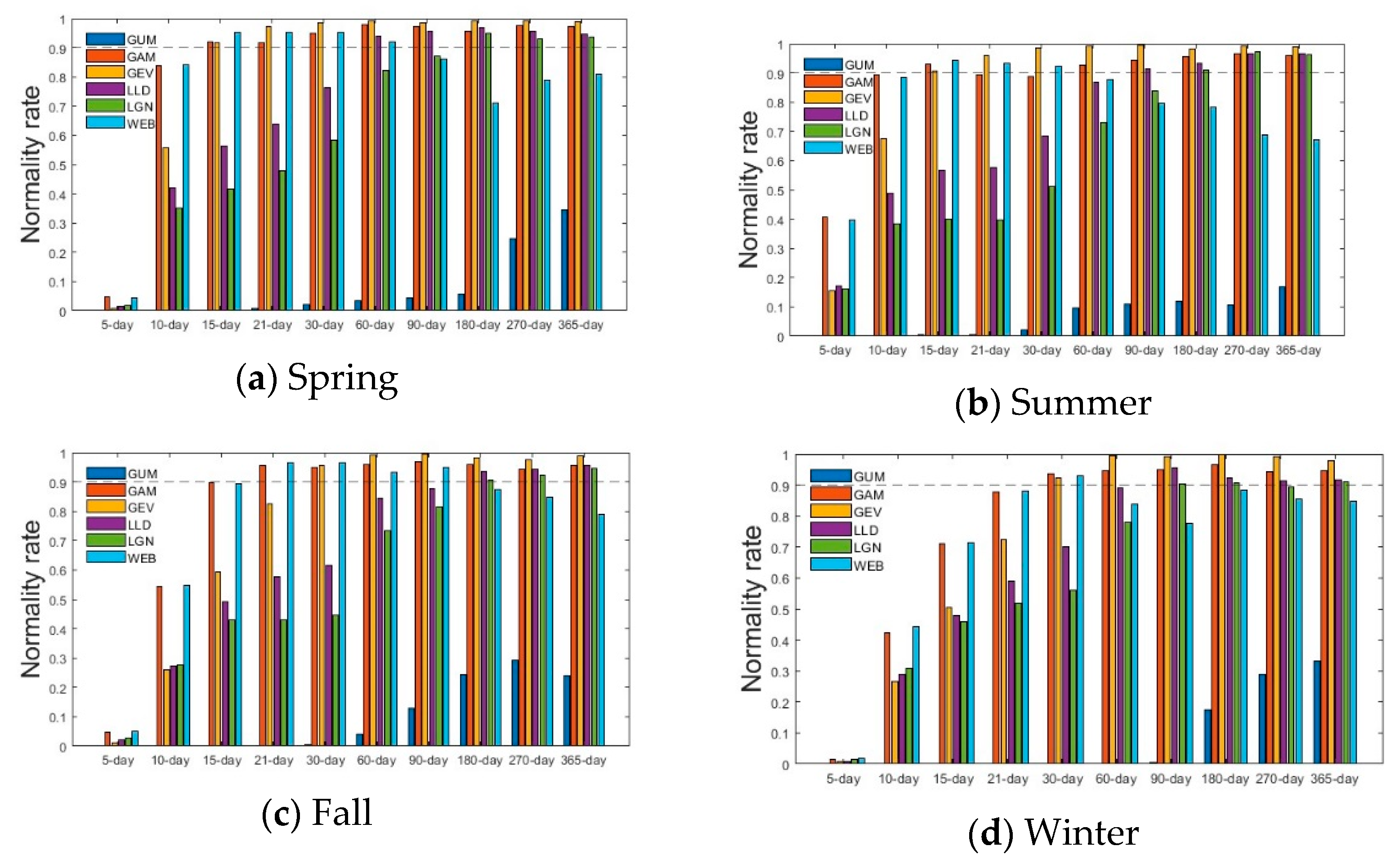
We used the Anderson–Darling test to determine if the SPI time series computed from the candidate PDFs followed a standard normal distribution. To test for normality, we calculated the proportion (i.e., normality ratio) of sites satisfying the normal distribution among all the sites for each season (see Figure 3). Wang et al. [16] assumed that if the normality ratio is greater than 90%, the time-series data of the region are normally distributed, and we also used this criterion to determine the normality of the SPI time series calculated for the corresponding time-scale.
As shown in Figure 3, we find that GUM is not applicable for any time-scales, regardless of season. GAM has a high normality ratio compared to the other PDFs for all time-scales. GEV has a lower normality ratio than GAM and WEB for short time-scales, but for longer time-scales it has a higher normality ratio than all the other candidate PDFs. WEB has a high normality ratio along with GAM for short time-scales, but the normality ratio decreases for time-scales longer than 60 days. As a result, we can say that GAM is a good representation of the normal distribution for all time-scales except for very short time-scales.
If we look at the results of the normality test separately for each season, we can see that there is a difference in the minimum time-scale that can be applied for each season. In spring, when calculating the SPI using GAM, GEV, and WEB, the time-scale can be reduced to 15 days, which means that the SPI can be obtained for a relatively short time-scale in the spring and still follow a normal distribution. In summer, as in spring, GAM, GEV, and WEB can be applied for a time-scale of 15 days. In the fall, the normality ratio is higher than 0.9 for a 21-day time-scale using GAM and WEB. Finally, in winter, we can say that a 30-day time-scale using GAM, GEV, and WEB is the minimum time-scale that can be applied. To summarize, the minimum time-scale for each season is 15 days in the spring and summer, 21 days in the fall, and 30 days in the winter. This means that it is possible to monitor changes in meteorological drought at relatively short time-scales in the spring and summer, but only at relatively long time-scales in the fall and winter.
Furthermore, looking at the regional results in Figures S21–S26 in the Supplementary Materials, the Gangwon region has a higher normality ratio than the results of all the regions combined (i.e., Figure 3), and the results of GAM are clearly superior for all time-scales in all seasons. In the Honam region, the normality ratio drops overall at long time-scales in the fall and winter, and GEV is the most stable distribution for time-scales above 30 day for all seasons.
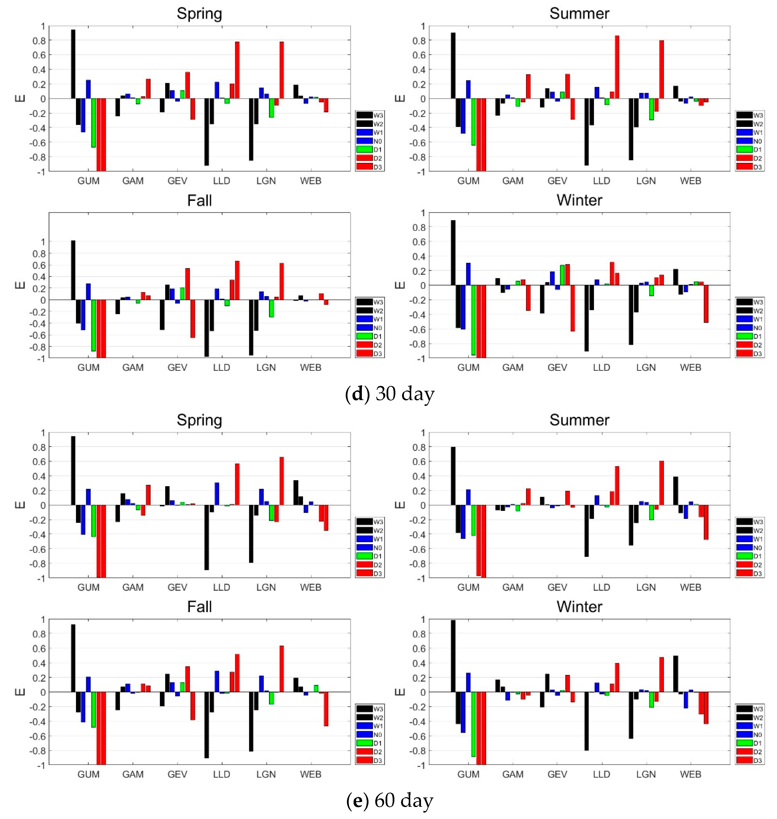
The Anderson–Darling test looks at whether the overall frequency shape of the SPI time series follows a normal distribution, but when analyzing drought with SPI, we are more interested in extreme drought events. In other words, it is important to see if the tails of the distribution follow a normal distribution. Therefore, we additionally assessed normality with E , the error rate of the SPI time series relative to the normal distribution. We compared the theoretical probability of occurrence for the drought classes in the SPI to the actual probability in the actual SPI time series. Figure 4 shows the error rate from the normal distribution corresponding to the drought classes of SPI at each time-scale (10 days, 15 days, 21 days, 30 days, and 60 days) for all seasons at all sites.
GUM has a very large E for all time-scales. GAM shows consistently good normality results compared to the other PDFs for all time-scales. WEB performs well for short time-scales. However, at a time-scale of 60 days, E becomes significantly larger.
Seasonally, the differences between seasons are evident for each time-scale. The SPI at a time-scale of 10 days shows very large error rates for drought classes D2 and D3 for all seasons except summer. This suggests that the time-scale of 10 days SPI is not a good representation of extreme drought because the cumulative-precipitation time series contains too many zero precipitation events. In summer, the SPIs for a time-scale of 10 days computed from GAM and WEB are relatively close to the normal distribution for the remaining drought classes, except for D3. From a time-scale of 15 days, the error rate decreases significantly and we can recognize that the distribution is becoming more normal. The error rate of D3 is still large in fall and winter, but in spring and summer the error rate of D3 decreases significantly to below 0.5. At this time-scale, GAM and WEB have significantly smaller error rates than the other candidate PDFs. At time-scales longer than 21 days, the seasonal results were different for the different PDFs. The 21-day GAM and WEB show lower error rates in the spring and summer and, in particular, the distribution of SPI by WEB follows a nearly perfect normal distribution. On the other hand, LLD and LGN show low error rates in the fall and winter. For the time-scale of 30 days, GAM and WEB have relatively low error rates in the summer and fall, GEV in the spring and summer, and LLD and LGN in the fall and winter. It is also worth noting that WEB has a very large error rate for D3 in winter. For the time-scale of 60 days, GAM has lower error rates in the fall and winter, and GEV in the spring and summer. The rest of the PDFs have similar error rates regardless of the season. To summarize, when trying to estimate the SPI for time-scales of 60 days or less, GAM had a lower error rate in the summer, and GEV and WEB had lower error rates in the spring and summer. Conversely, LLD and LGN had lower error rates in the fall and winter.
We show the seasonal error rates across all the sites for each time-scale (5 day, 90 day, 180 day, 270 day, 365 day) in Figures S27–S31 in the Supplementary Materials. The 5 day does not adequately reflect D2 and D3 in summer nor D1, D2, and D3 for the rest of the seasons (see Figure S27). For the 90 day and 180 day, GAM and GEV show good normality in the spring and summer, with large error rates in the fall (see Figures S28 and S29). Similar to the 90 day, the 180 day shows good normality of GAM and GEV in the spring and summer (Figure S29). For the 270 day and 365 day, we find no significant difference in the error rates of GAM, GEV, and LGN (see Figures S30 and S31). It is also worth noting that when the time-scales are longer than 270 days, the error rate of GAM and GEV increases, while the error rate of LGN decreases.

4. Discussion

4.1. Effect of Zero Precipitation Events on Minimum Time-Scales

As flush droughts become more frequent, the need for short-term drought assessments is increasing. However, the monthly SPI currently in use has difficulty responding to such flush droughts. There is a need for a method to accurately capture droughts that develop rapidly in a short period of time. As part of this, the need to apply a daily time-scale SPI is increasing.
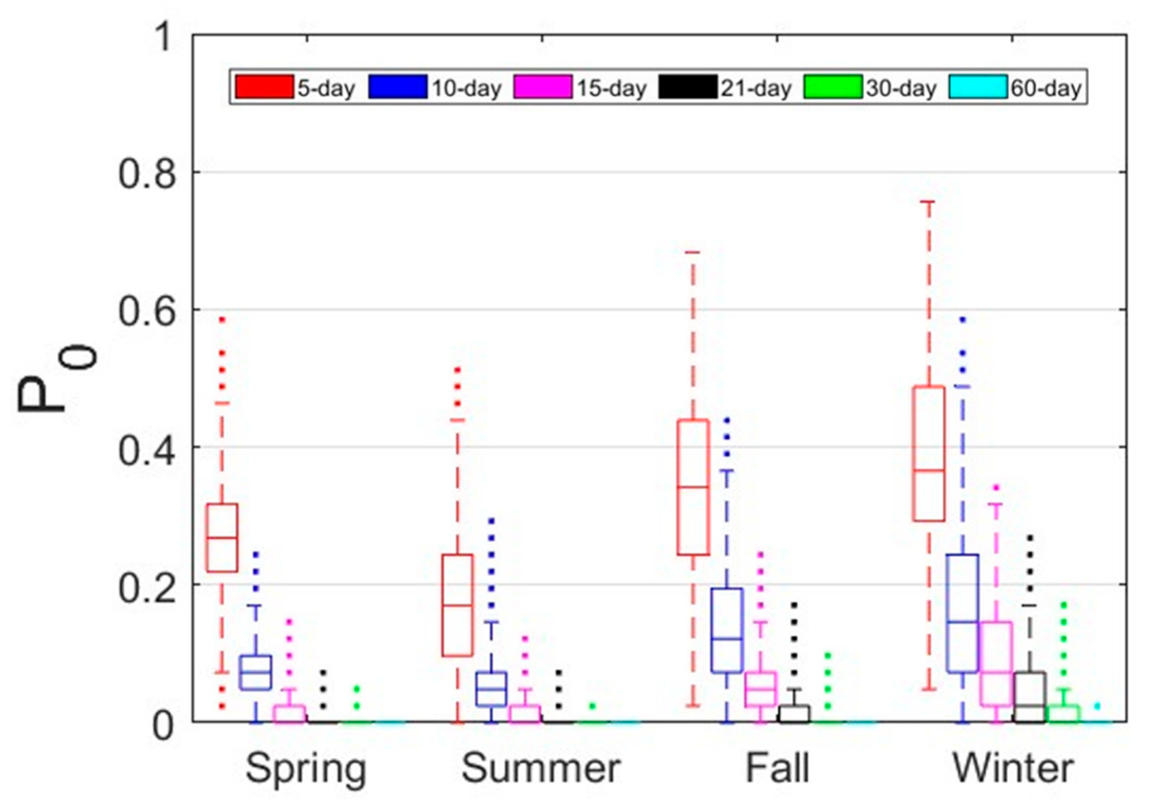
Yoo et al. [33] suggested the use of daily SPIs because SPIs calculated for a monthly time-scale have poor reproducibility for suddenly occurring extreme drought events. Wang et al. [16] also mentioned the need for daily SPIs, noting that SPIs for longer time-scales are insensitive to short-term changes in precipitation, making it difficult to identify the beginning and end of a drought event and to monitor suddenly occurring droughts in detail. However, in order to apply the daily SPI to a short time-scale, it is necessary to take into account the fact that the cumulative-precipitation time series contains many zero values (see Figure 5).
In South Korea, there is a large seasonal variation in precipitation, with more than half of the average annual precipitation concentrated in the summer. Due to this characteristic, the proportion of zero values in the cumulative-precipitation time series in summer is the lowest among the four seasons. Conversely, due to the dry nature of the winter climate, the percentage of zero values in the cumulative-precipitation time series is the highest in winter. For spring and fall, the percentage of zeros in the cumulative-precipitation time series is higher in the fall, even though fall precipitation is slightly higher. This fact is directly related to the results of the normality test.
In this study, the Anderson–Darling test and a deviation from N 0,1 were performed to test for normality. In the Anderson–Darling test, a normality ratio of 0.9 or higher is set as the criterion for the minimum-applicable time-scale [16]. Under the premise of using the probability distribution with the best normality, from Figure 3, the minimum time-scales with a normality ratio of 0.9 or higher are 15 day, 21 day, and 30 day in the order of spring, summer, fall, and winter, which is consistent with the results in Figure 5. In addition, GAM and WEB in Figure 4b show good normality in the spring and summer. For fall and winter, we find that the error rates at 21 days and 30 days, respectively, decrease to a similar extent as the error rates in spring and summer at 15 days. When the proportion of zero values is high in a moving cumulative-precipitation time series, a significant lower bound is introduced in the SPI calculation, resulting in a truncation of the SPI distribution [7,25]. The proportion of zero values in the time series of moving accumulated precipitation over South Korea is highly seasonal, which also imposes seasonal differences on the minimum time-scale for calculating the SPI. As mentioned in Wu et al. [25], WMO [11], and Wang et al. [16], it is difficult to apply SPI with a short time-scale to the winter in South Korea, which is a period of low precipitation. Wang et al. [16] suggested that it is reasonable to apply a longer minimum time-scale in arid regions compared to humid regions. This is consistent with the longer minimum time-scale in the relatively dry Chungcheong region, a region with a high proportion of zero cumulative-precipitation values.
This can also be seen in the regional results. From Figure S32c in the Supplementary Materials, we can see that the proportion of zero values is high in the fall and winter in the Chungcheong region. The results of the normality test for fall and winter in this region are shown in Figure S26c,d in the Supplementary Materials. It can be seen that the normality test results for autumn and winter in this region have a significantly lower normality ratio than the rest of the regions, which means that the high proportion of zero values in the precipitation time series in the Chungcheon region causes the SPI time series to deviate from the normal distribution.
One interesting fact is the normality ratio for the summer season in the Gangwon region (Figure S21 in the Supplementary Materials). The normality ratio of 0.9 is satisfied at a time-scale of 10 days, and a time-scale of 10 days is the shortest applicable time-scale among all the SPI time series analyzed in this study. The median proportion of zero values for 10 days in summer in the Gangwon region is 0.0244, which is lower than that of the other regions (see Figure S32 in the Supplementary Materials). By examining the proportion of zeros in each region, we can see that the normality ratio exceeds 0.9 at the boundary of 0.0244, meaning that if the cumulative-precipitation time series has less than 2.5% zeros, we can conclude that the corresponding SPI time series is normally distributed.
From Figure 5, we can see that the shorter the time-scale, the higher the percentage of zero values and, from Figure 3, we can see that all the PDFs have low normality ratios for short time-scales. Overall, all the PDFs have low normality ratios for short time-scales, but GAM and WEB have relatively high normality ratios among the PDFs. Similar results can be found in Stagge et al. [7]. Stagge et al. [7] reported that for short time-scales, WEB and GAM exhibited low rejection rates among the candidate PDFs, with WEB and GAM performing best in that order. However, in our study, we found that the performance of WEB deteriorates rapidly as the time-scale increases. GAM performed well for all time-scales and was found to be the optimal probability distribution for calculating the daily SPI. However, if a minimum time-scale SPI is required for a specific purpose, it may be preferable to calculate the SPI using WEB.
In this study, the proportion of zero values was applied as the probability mass of zero cumulative precipitation (see Equation (1)). Therefore, when the probability mass is above a certain level, the frequency distribution of the SPI time series is bound to deviate from the normal distribution [7]. As a result, the accuracy of the normality of the SPI calculated by including zero values decreases, making it unreasonable to use it on short time-scales [9]. Currently, there is no standardized method for ensuring the normality of SPI by accounting for the proportion of zero values in SPI calculations, so further research is needed.

4.2. Applicability of the GEV Distribution

Globally, the most commonly applied PDF for SPI computation is GAM. As shown in McKee et al., Stagge et al., Okpara et al., Blain et al., and Zhao et al. [1,7,8,9,20], GAM is used worldwide. Also, in South Korea, GAM is currently used for PDF [34,35,36]. However, these facts are only valid for a monthly time-scale. It is not easy to find studies on whether GAM is the optimal probability distribution for calculating the SPI for a daily time-scale in South Korea or globally.
GAM is often used because the expression structure of its distribution is relatively simple, and cumulative-precipitation time series around the world have been shown to generally follow GAM. It has been reported that cumulative-precipitation time series in South Korea also follow GAM [35]. In this study, the Chi-square test indicates that overall, GAM is the best probability distribution when evaluated for all time-scales (see Table 2).
The AIC test still shows that GAM performs best for all time-scales (see Figure 2). However, GEV’s performance under an AIC distribution improves dramatically as the time-scale gets progressively longer (e.g., 365 day). In addition, the normality test shows that GEV performs very well when the time-scale is longer than 30 days (see Figure 3). However, this is not evidence that GEV is superior to GAM. From Figure 4, which shows the deviation from the normal distribution in the drought class, we cannot say that GEV performs better than GAM at time-scales greater than 30 days. In addition, although GEV is flexible in calculating SPI, it has risks, such as the uncertainty caused by the addition of one more distributional parameter and the constraints on the upper or lower bound of the time series imposed by the sign of the shape parameter. Since GEVs are often faced with these inconveniences in practical applications, two-parameter probability distributions are often applied in practice [7,37]. In addition, DeGaetano et al. and Carbone et al. [38,39] reported that record lengths of at least 60 years are required to estimate stable parameters and, hence, calculate reliable SPIs. Guttman and Wang et al. [2,16] also recommended a record length of 70 years or more for SPI calculation. Considering the current record length of about 40 years, the application of a three-parameter probability distribution such as the GEV would be unreasonable. In addition, since the goodness-of-fit test is performed using data excluding zero values, the actual record length will be shorter when estimating the parameters of the probability distribution for calculating SPI on shorter time-scales, leading to greater uncertainty in the SPI calculation [25]. For these reasons, it is difficult to say that GEV is a better probability distribution for SPI calculation in South Korea compared to GAM, although there are many precipitation time series that show that GEV performs well in terms of goodness-of-fit and normality of distribution.

5. Conclusions

The SPI is a standardized index of precipitation variability, and the probability distribution used to calculate the SPI in many studies is typically Gamma. In addition, the SPI is mainly used to evaluate drought on a monthly time-scale. However, in principle, it is necessary to select and apply the most appropriate probability distribution to the precipitation time series to calculate the SPI, and the need for a daily time-scale is emerging as concerns about fresh drought have increased in recent years. In this study, we investigated the optimal probability distribution for calculating SPI at sub-daily time-scales and the minimum time-scale that could be applied using daily precipitation time series observed for 42 years at 56 sites in South Korea.
The results of the chi-square goodness-of-fit test and the AIC show that GAM is the best-overall probability distribution for short time-scales (30 days or less) to long time-scales (365 days). However, we also found that WEB slightly outperforms GAM for short time-scales of 60 days or less. The AIC test suggests that GEV performs well at longer time-scales of 180 days or more, but the normality test does not provide evidence that GEV is a better distribution than GAM. We also found that the proportion of zeros in a precipitation time series has a decisive effect on the normality test, and this is more evident when calculating the SPI at short time-scales of 30 days or less.
While there are some regional differences, the minimum time-scale for calculating the daily SPI in South Korea varies by season as follows: 15 days for spring and summer, 21 day for fall, and 30 days for winter. The factor that most influenced the minimum time-scale was the share of zero events in the cumulative-precipitation time series, which was found to be appropriate for calculating the SPI if it was 2.5% or less. The best distribution for calculating SPI is WEB for time-scales below 60 days and GAM for all other time-scales, and if we had to choose one probability distribution that could be applied across all time-scales, we would recommend GAM.
Our findings clearly contain limitations and uncertainties, including data quality and availability, parameter-estimation methods, and spatial variability of precipitation. It would also be worthwhile to extend our investigation in the future by utilizing other PDFs or other drought indices, applying other transformation methods, or incorporating other climate factors.

Supplementary Materials

The following supporting information can be downloaded at: https://www.mdpi.com/article/10.3390/atmos14081292/s1, Figure S1: Box-plot of the p -values of the chi-square test for six candidate PDFs for the four seasons in the Gangwon region; Figure S2: Box-plot of the p -values of the chi-square test for six candidate PDFs for the four seasons in the Capital region; Figure S3: Box-plot of the p -values of the chi-square test for six candidate PDFs for the four seasons in the Buulgyeong region; Figure S4: Box-plot of the p -values of the chi-square test for six candidate PDFs for the four seasons in the Daegyeong region; Figure S5: Box-plot of the p -values of the chi-square test for six candidate PDFs for the four seasons in the Honam region; Figure S6: Box-plot of the p -values of the chi-square test for six candidate PDFs for the four seasons in the Chungcheong region; Figure S7: Heatmap of h   (%) of the chi-square test for six candidate PDFs for the four seasons; Figure S8: Heatmap of p   (%) of the chi-square test for six candidate PDFs for the four seasons; Figure S9: Heatmap of w   (%) of the chi-square test for six candidate PDFs for the four seasons; Figure S10: AIC frequencies for candidate PDFs in the Gangwon region; Figure S11: AIC frequencies for candidate PDFs in the Capital region; Figure S12: AIC frequencies for candidate PDFs in the Buulgyeong region; Figure S13: AIC frequencies for candidate PDFs in the Daegyeong region; Figure S14: AIC frequencies for candidate PDFs in the Honam region; Figure S15: AIC frequencies for candidate PDFs in the Chungcheong region; Figure S16: AIC frequencies for candidate PDFs in the spring season; Figure S17: AIC frequencies for candidate PDFs in the summer season; Figure S18: AIC frequencies for candidate PDFs in the fall season; Figure S19: AIC frequencies for candidate PDFs in the winter season; Figure S20: A box-plot showing A I C D values for each probability distribution by time-scale; Figure S21: Normality ratio for six candidate PDFs for all seasons in the Gangwon region; Figure S22: Normality ratio for six candidate PDFs for all seasons in the Capital region; Figure S23: Normality ratio for six candidate PDFs for all seasons in the Buulgyeong region; Figure S24: Normality ratio for six candidate PDFs for all seasons in the Daegyeong region; Figure S25: Normality ratio for six candidate PDFs for all seasons in the Honam region; Figure S26: Normality ratio for six candidate PDFs for all seasons in the Chungcheong region; Figure S27: Error rate of SPI at 5 days calculated per drought class for all seasons across all sites; Figure S28: Error rate of SPI at 90 days calculated per drought class for all seasons across all sites; Figure S29: Error rate of SPI at 180 days calculated per drought class for all seasons across all sites; Figure S30: Error rate of SPI at 270 days calculated per drought class for all seasons across all sites; Figure S31: Error rate of SPI at 365 days calculated per drought class for all seasons across all sites; Figure S32: Rate of cumulative time series having zero value for all seasons at each time-scale (5 day, 10 day, 15 day, 21 day, 30 day, and 60 day) for each region.

Author Contributions

Conceptualization, C.L. and S.K.; methodology, C.L. and S.K.; software, C.L. and S.K.; validation, C.L. and J.S.; formal analysis, C.L. and S.K.; Investigation, C.L. and S.K.; resources, J.W.; writing—original draft preparation, C.L. and S.K.; writing—review and editing, J.S. and J.W.; visualization, J.W. and J.S.; supervision, J.S.; project administration, S.K.; funding acquisition, S.K. All authors have read and agreed to the published version of the manuscript.

Funding

This work was supported by the Korea Environment Industry & Technology Institute (KEITI) through the Water Management Program for Drought Project, funded by the Korea Ministry of Environment (MOE) (202305020001).

Institutional Review Board Statement

Not applicable.

Informed Consent Statement

Not applicable.

Data Availability Statement

Not applicable.

Conflicts of Interest

The authors declare no conflict of interest.

References

  1. McKee, T.B.; Doesken, N.J.; Kleist, J. The relationship of drought frequency and duration to time scales. In Proceedings of the 8th Conference on Applied Climatology, Boston, MA, USA, 17–22 January 1993; Volume 17, pp. 179–183. [Google Scholar]
  2. Guttman, N.B. Accepting the standardized precipitation index: A calculation algorithm. J. Am. Water Resour. Assoc. 1999, 35, 311–322. [Google Scholar] [CrossRef]
  3. Kyoung, M.; Kim, S.; Kim, B.; Kim, H. Construction of hydrological drought severity-area-duration curves using cluster analysis. KSCE J. Civ. Environ. Eng. Res. 2007, 27, 267–276. [Google Scholar]
  4. Kim, H.; Park, J.; Yoon, J.; Kim, S. Application of SAD curves in assessing climate-change impacts on spatio-temporal characteristics of extreme drought events. KSCE J. Civ. Environ. Eng. Res. 2010, 30, 561–569. [Google Scholar]
  5. Sienz, F.; Bothe, O.; Fraedrich, K. Monitoring and quantifying future climate projections of dryness and wetness extremes: SPI bias. Hydrol. Earth Syst. Sci. 2012, 16, 2143–2157. [Google Scholar] [CrossRef]
  6. Wang, Y.; Li, J.; Feng, P.; Hu, P. A time-dependent drought index for non-stationary precipitation series. Water Resour. Manag. 2015, 29, 5631–5647. [Google Scholar] [CrossRef]
  7. Stagge, J.H.; Tallaksen, L.M.; Gudmundsson, L.; Van Loon, A.F.; Stahl, K. Candidate distributions for climatological drought indices (SPI and SPEI). Int. J. Climatol. 2015, 35, 4027–4040. [Google Scholar] [CrossRef]
  8. Okpara, J.; Afiesimama, E.; Anuforom, A.; Owino, A.; Ogunjobi, K. The applicability of standardized precipitation index: Drought characterization for early warning system and weather index insurance in West Africa. Nat. Hazards 2017, 89, 555–583. [Google Scholar] [CrossRef]
  9. Blain, G.C.; de Avila, A.M.H.; Pereira, V.R. Using the normality assumption to calculate probability-based standardized drought indices: Selection criteria with emphases on typical events. Int. J. Climatol. 2018, 38, e418–e436. [Google Scholar] [CrossRef]
  10. Guenang, G.; Komkoua, M.; Pokam, M.; Tanessong, R.; Tchakoutio, S.; Vondou, A.; Tamoffo, A.; Djiotang, L.; Yepdo, Z.; Mkankam, K. Sensitivity of SPI to Distribution Functions and Correlation Between its Values at Different Time Scales in Central Africa. Earth Syst. Environ. 2019, 3, 203–214. [Google Scholar] [CrossRef]
  11. Svoboda, M.; Hayes, M.; Wood, D. Standardized Precipitation Index User Guide; World Meteorological Organization: Geneva, Switzerland, 2012.
  12. Chang, Y.; Kim, S.; Choi, G. A study of drought spatio-temporal characteristics using SPI-EOF analysis. J. Korea Water Resour. Assoc. 2006, 39, 691–702. [Google Scholar] [CrossRef]
  13. Paulo, A.; Martins, D.; Pereira, L.S. Influence of precipitation changes on the SPI and related drought severity. An analysis using long-term data series. Water Resour. Manag. 2016, 30, 5737–5757. [Google Scholar] [CrossRef]
  14. Sim, H.; Ryu, J.; Ahn, J.; Kim, J.; Kim, S. Real-time drought index for determining drought conditions in natural water supply system communities. J. Korean Soc. Hazard Mitig. 2013, 13, 365–374. [Google Scholar] [CrossRef]
  15. Won, J.; Jang, S.; Kim, K.; Kim, S. Applicability of the evaporative demand drought index. J. Korean Soc. Hazard Mitig. 2018, 18, 431–442. [Google Scholar] [CrossRef]
  16. Wang, W.; Wang, J.; Romanowicz, R. Uncertainty in SPI calculation and its impact on drought assessment in different climate regions over China. J. Hydrometeorol. 2021, 22, 1369–1383. [Google Scholar] [CrossRef]
  17. Park, B.; Lee, J.; Kim, C.; Jang, H. Projection of future drought of Korea based on probabilistic approach using multi-model and multi climate change scenarios. KSCE J. Civ. Eng. Res. 2013, 33, 1871–1885. [Google Scholar] [CrossRef]
  18. Park, M.; Lee, O.; Park, Y.; Kim, S. Future drought projection In Korea under ar5 rcp climate change scenarios. J. Korean Soc. Hazard Mitig. 2015, 15, 423–433. [Google Scholar] [CrossRef]
  19. Kim, B.; Chang, I.; Sung, J.; Han, H. Projection in Future Drought Hazard of South Korea Based on RCP Climate Change Scenario 8.5 Using SPEI. Adv. Meteorol. 2016, 2016, 4148710. [Google Scholar] [CrossRef]
  20. Zhao, R.; Wang, H.; Zhan, C.; Hu, S.; Ma, M.; Dong, Y. Comparative analysis of probability distributions for the Standardized Precipitation Index and drought evolution in China during. Theor. Appl. Climatol. 2020, 139, 1363–1377. [Google Scholar] [CrossRef]
  21. Angelidis, P.; Maris, F.; Kotsovinos, N.; Hrissanthou, V. Computation of drought index SPI with alternative distribution functions. Water Resour. Manag. 2012, 26, 2453–2473. [Google Scholar] [CrossRef]
  22. Pieper, P.; Dusterhus, A.; Baehr, J. A universal Standardized Precipitation Index candidate distribution function for observations and simulations. Hydrol. Earth Syst. Sci. 2020, 24, 4541–4565. [Google Scholar] [CrossRef]
  23. Kim, B.; Kim, S.; Lee, J.; Kim, H. Spatio-temporal characteristics of droughts in Korea: Construction of drought severity-area-duration curves. KSCE J. Civ. Environ. Eng. Res. 2006, 26, 69–78. [Google Scholar]
  24. Ryu, J.; Ahn, J.; Kim, S. An application of drought severity-area-duration curves using copulas-based joint drought index. J. Korea Water Resour. Assoc. 2012, 45, 1043–1050. [Google Scholar] [CrossRef]
  25. Wu, H.; Svoboda, M.D.; Hayes, M.J.; Wilhite, D.A.; Wen, F. Appropriate application of the Standardized Precipitation Index in arid locations and dry seasons. Int. J. Climatol. 2007, 27, 65–79. [Google Scholar] [CrossRef]
  26. Spinoni, J.; Naumann, G.; Carrao, H.; Barbosa, P.; Vogt, J. World drought frequency, duration, and severity for 1951–2010. Int. J. Climatol. 2014, 34, 2792–2804. [Google Scholar] [CrossRef]
  27. Pearson, K. On the criterion that a given system of deviations from the probable in the case of a correlated system of variables is such that it can be reasonably supposed to have arisen from random sampling. Lond. Edinb. Dublin Philos. Mag. J. Sci. 1900, 50, 157–175. [Google Scholar] [CrossRef]
  28. Akaike, H. A new look at the statistical model identification. IEEE Trans. Autom. Control 1974, 19, 716–723. [Google Scholar] [CrossRef]
  29. Akaike, H. Information Theory and an Extension of the Maximum Likelihood Principle. In Selected Papers of Hirotugu Akaike; Springer: New York, NY, USA, 1998; pp. 199–213. [Google Scholar]
  30. Anderson, T.; Darling, D. A Test of Goodness of Fit. J. Am. Stat. Assoc. 1954, 49, 765–769. [Google Scholar] [CrossRef]
  31. Burnham, K.P.; Anderson, D.R. Model Selection and Multi-Model Inference: A Practical Information-Theoretical Approacrh, 2nd ed.; Springer: New York, NY, USA, 2002. [Google Scholar]
  32. Lee, O.; Sim, I.; Kim, S. Application of the non-stationary peak-over-threshold methods for deriving rainfall extremes from temperature projections. J. Hydrol. 2020, 585, 124318. [Google Scholar] [CrossRef]
  33. Yoo, J.; Song, H.; Kim, T.; Ahn, J. Evaluation of Short-Term Drought Using Daily Standardized Precipitation Index and ROC Analysis. J. Korean Soc. Civ. Eng. 2013, 33, 1851–1860. [Google Scholar] [CrossRef]
  34. Kim, S.; Kim, B.; Ahn, T.; Kim, H. Spatio-temporal characterization of Korean drought using severity-area–duration curve analysis. Water Environ. J. 2011, 25, 22–30. [Google Scholar] [CrossRef]
  35. Kang, D.; Nam, D.; Kim, B. Comparison of Meteorological Drought Indices Using Past Drought Cases of Taebaek and Sokcho. J. Korean Soc. Civ. Eng. 2019, 39, 735–742. [Google Scholar]
  36. Won, J.; Choi, J.; Lee, L.; Kim, S. Copula-based Joint Drought Index using SPI and EDDI and its application to climate change. Sci. Total Environ. 2020, 744, 140701. [Google Scholar] [CrossRef] [PubMed]
  37. Lloyd-Hughes, B.; Saunders, M.A. A drought climatology for Europe. Int. J. Climatol. 2002, 22, 1571–1592. [Google Scholar] [CrossRef]
  38. DeGaetano, A.T.; Belcher, B.N.; Noon, W. Temporal and spatial interpolation of the standardized precipitation index for computational efficiency in the dynamic drought index tool. J. Appl. Meteorol. Climatol. 2015, 54, 795–810. [Google Scholar] [CrossRef]
  39. Carbone, G.J.; Lu, J.; Brunetti, M. Estimating uncertainty associated with the standardized precipitation index. Int. J. Climatol. 2018, 38, e607–e616. [Google Scholar] [CrossRef]
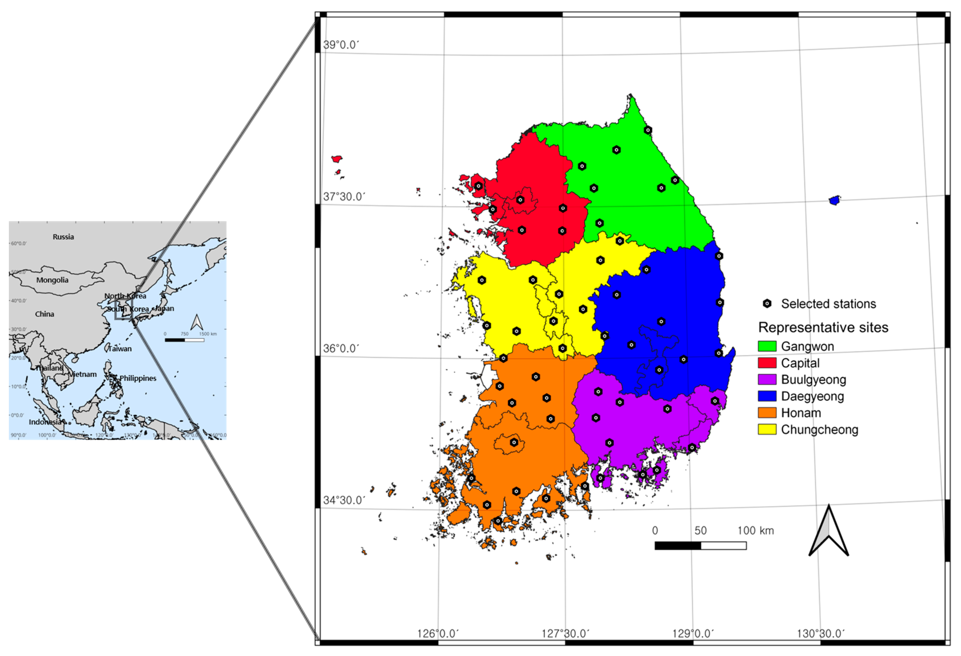
Figure 1. Location of precipitation observation sites.
Atmosphere 14 01292 g001
Figure 2. AIC frequencies for candidate PDFs.
Atmosphere 14 01292 g002
Figure 3. Normality ratio for six candidate PDFs per season across all sites.
Atmosphere 14 01292 g003
Figure 4. Error rate of SPI calculated per drought class for all seasons across all sites.
Atmosphere 14 01292 g004aAtmosphere 14 01292 g004b
Figure 5. Rate of cumulative time series having zero values in all seasons for each time-scale (5 day, 10 day, 15 day, 21 day, 30 day, and 60 day) in the entire region.
Atmosphere 14 01292 g005
Table 1. Drought classification in SPI.
SPI IntervalPeriod ClassificationProbability
SPI ≥ 2W3: extremely wet0.0228
2 > SPI ≥ 1.5W2: severely wet0.0441
1.5 > SPI ≥ 1W1: moderately wet0.0918
1 > SPI > −1N0: normal0.6827
−1 ≥ SPI > −1.5D1: moderately dry0.0918
−1.5 ≥ SPI > −2D2: severely dry0.0441
SPI ≤ −2D3: extremely dry0.0228
Table 2. The mean The mean p-values and the acceptable and win rates of the candidate PDFs. The colored cells indicate the best performance among the candidate PDFs.
Time-Scale5 Day10 Day15 Day
SeasonPDF Mean   p h (%) w (%) Mean   p h (%) w (%) Mean   p h (%) w (%)
SpringGUM0.069822.86498.67620.051522.86496.50230.046521.37035.4542
GAM0.438789.033442.48840.331089.033424.90300.313889.518615.6250
GEV0.233176.59164.83310.284376.591623.07840.303683.132828.7849
LLD0.267071.23455.22130.231971.23458.88980.255178.862612.3253
LGN0.232657.43405.35710.163157.43404.85250.174863.31526.9682
WEB0.448089.712733.42390.346289.712731.77410.332290.508530.8424
SummerGUM0.039315.10095.31830.031915.10094.23140.036016.90613.9790
GAM0.408288.781144.48760.340388.781127.50390.304087.597017.1584
GEV0.222475.95117.76400.281175.951121.87500.309282.764032.4728
LLD0.255875.03886.71580.255775.038811.97590.256279.192513.5481
LGN0.217460.63665.86180.185660.63666.26940.170462.71356.7547
WEB0.423490.081529.85250.354990.081528.14440.317789.072226.0870
FallGUM0.058415.89486.29910.029215.89483.61070.029615.26693.6303
GAM0.406591.876042.85710.395491.876043.21040.358390.541631.8681
GEV0.203862.24491.92310.209362.24497.14290.258072.900317.7983
LLD0.320174.52908.35950.267674.52907.12320.265677.021211.3815
LGN0.319569.525112.04870.241269.52518.57540.213267.54326.8681
WEB0.439993.033828.51260.416193.033830.33750.376891.208828.4537
WinterGUM0.069917.34137.81750.036517.34134.94050.029113.69053.8492
GAM0.374289.384933.35320.367589.384931.64680.349789.027825.6746
GEV0.224067.24212.28170.241067.24217.40080.274974.027815.7540
LLD0.339778.392910.27780.309078.392910.07940.296678.492112.4405
LGN0.351876.567517.46030.301476.567515.19840.265372.757912.1429
WEB0.417191.845228.80950.401491.845230.73410.374091.150830.1389
Time-Scale30 Day60 Day90 Day
SeasonPDF Mean   p h   (%) w   (%) Mean   p h  (%) w   (%) Mean   p h   (%) w   (%)
SpringGUM0.051225.44642.58150.073038.74222.40680.076838.56752.7562
GAM0.315989.072215.31440.348092.158414.16930.354690.799715.9744
GEV0.283684.627321.37030.276985.578413.31520.265882.550511.8789
LLD0.293486.510119.73990.345091.983726.55280.348391.828427.1351
LGN0.219676.94109.99610.281786.801212.96580.307188.198816.4402
WEB0.337490.062130.99770.342690.333930.59010.322386.956525.8152
SummerGUM0.058228.47443.61020.083038.33463.26090.094442.91543.7655
GAM0.314987.732914.34390.334189.906814.79040.363792.158414.7710
GEV0.293385.015521.95260.258582.88049.33620.275184.84089.6079
LLD0.288584.336217.06130.326089.732125.56290.360892.352527.7174
LGN0.215772.61269.16150.256682.026410.48140.304188.101712.7329
WEB0.340489.635133.87030.341388.781136.56830.333686.840131.4053
FallGUM0.040419.46623.57140.080337.87283.78730.126058.06515.9066
GAM0.314188.500815.69860.343691.797512.99060.363693.485114.5801
GEV0.308685.145229.59180.302887.284118.95600.267885.53778.1240
LLD0.268181.652313.95210.327789.540820.17270.338691.856419.8980
LGN0.192769.01497.04470.268684.517312.06830.292688.029812.7551
WEB0.329489.266130.14130.357491.346232.02510.390993.367338.7363
WinterGUM0.01979.16671.44840.01669.34520.17860.037220.15871.2103
GAM0.314488.174616.01190.335890.992112.85710.343791.250015.0595
GEV0.352187.718334.46430.347389.007930.77380.311986.984123.3730
LLD0.303884.742115.53570.354591.984125.79370.345291.269823.4722
LGN0.242374.881010.43650.292284.285713.80950.304387.976216.0913
WEB0.314188.750022.10320.302087.341316.58730.304386.071420.7937
Time-Scale180 Day270 Day365 Day
SeasonPDF Mean   p h   (%) w   (%) Mean   p h   (%) w   (%) Mean   p h   (%) w   (%)
SpringGUM0.085141.20732.96970.150159.23915.90060.185467.29437.4534
GAM0.379692.954214.90680.379793.400617.70190.403092.954219.8758
GEV0.292586.024815.25620.278284.47209.10330.292585.73378.1716
LLD0.377094.002327.30980.363792.818324.76710.383792.896021.5062
LGN0.354391.944919.15760.333790.644415.10090.365291.595514.5380
WEB0.298484.394420.39980.342889.149827.42620.353489.130428.4550
SummerGUM0.101545.24464.48370.099145.26404.40610.154858.77166.5149
GAM0.367691.401417.48840.386493.458917.43010.403493.916821.5071
GEV0.249981.67707.23990.275784.87979.95730.292685.26308.2025
LLD0.359791.731429.44490.385493.963531.67700.387393.445827.0408
LGN0.325889.130413.27640.361192.488417.60480.354492.072210.5769
WEB0.314485.830728.06680.283083.385118.92470.333488.402726.1578
FallGUM0.164565.62017.22140.171265.09037.63340.187968.09526.8452
GAM0.401691.895619.15230.394092.425417.52350.386491.746019.7024
GEV0.281984.49762.82570.274484.06593.53220.284182.77787.4008
LLD0.377091.974122.84140.365692.445126.00080.352691.170622.5992
LGN0.344790.051013.99140.342590.306111.36190.335488.670610.9325
WEB0.376689.619333.96780.364688.206433.94820.356189.504032.5198
WinterGUM0.129955.31755.09920.153160.93256.11110.153160.93256.1111
GAM0.367192.579414.36510.349389.226216.21030.349389.226216.2103
GEV0.278585.734111.17060.255678.98815.09920.255678.98815.0992
LLD0.342891.726216.86510.334588.928621.09130.334588.928621.0913
LGN0.329890.734117.04370.312885.853212.32140.312885.853212.3214
WEB0.367992.103235.45630.341588.829439.16670.341588.829439.1667
Table 3. r-values at A I C D m a x = 2 for GAM and WEB for short time-scales.
Time-Scale5 Day10 Day15 Day21 Day30 Day
PDF
GAM0.85490.93030.93180.89450.8532
WEB0.90360.95260.95630.93460.8879
Disclaimer/Publisher’s Note: The statements, opinions and data contained in all publications are solely those of the individual author(s) and contributor(s) and not of MDPI and/or the editor(s). MDPI and/or the editor(s) disclaim responsibility for any injury to people or property resulting from any ideas, methods, instructions or products referred to in the content.