Article

Future Implications of Climate Change on Arum palaestinum Boiss: Drought Tolerance, Growth and Production

1
Department of Forest & Rangeland Stewardship, Warner College of Natural Resources, Colorado State University, Fort Collins, CO 80523, USA
2
Department of Natural Resources, Faculty of African Postgraduate Studies, Cairo University, Giza 12613, Egypt
3
Department of Atmospheric Physics, Earth Science Institute, Slovak Academy of Sciences, 840 05 Bratislava, Slovakia
*
Author to whom correspondence should be addressed.
Atmosphere 2023, 14(9), 1361; https://doi.org/10.3390/atmos14091361
Submission received: 25 June 2023 / Revised: 25 August 2023 / Accepted: 26 August 2023 / Published: 29 August 2023

Abstract

:
The objectives of the work were to understand the potential future climate changes in the Mediterranean region, assess the drought tolerance of the black calla lily (Arum palaestinum Boiss.), and investigate the mechanisms associated with its ability to withstand drought conditions. The Shared Socioeconomic Pathways (SSPs) of the Intergovernmental Panel on Climate Change (IPCC) were used to predict future temperature and precipitation changes. Both the SSP2-4.5 and SSP5-8.5 scenarios predicted a general increase in minimum and maximum temperatures and a decrease in precipitation. The projected increase in minimum temperature ranged from 2.95 °C under SSP2-4.5 to 5.67 °C under SSP5-8.5. The projected increase in maximum temperature ranged from 0.69 °C under SSP2-4.5 to 3.34 °C under SSP5-8.5. The projected decrease in precipitation ranged from −1.04 mm/day under SSP2-4.5 to −1.11 mm/day under SSP5-8.5. Results indicated that drought significantly impacted the physiological responses of the black calla lily. As drought increased, the black calla lily showed a reduction in leaf characteristics and non-structural carbohydrates, while proline content and reducing sugar content were increased, enhancing drought tolerance through osmoregulation. The black calla lily tolerates drought at a total ET of up to 50%. It has the potential to adapt to expected climate change through osmoregulation or by building a carbon and nitrogen sink for stress recovery.

1. Introduction

Climate change has become one of the supreme contests to natural ecosystems processing and dynamics. Variations in seasonal patterns, temperature varieties, rainfall uniformity, and other associated phenomena have been described and attributed to global climate change [1]. With the continuity of harmful human activities such as overpopulation, pollution, fossil fuel burning, and deforestation, negative impacts can be triggered. These impacts include climate change, soil erosion, poor air quality, and undrinkable water. The harmful impacts of climate change will become much stronger and more harmful in the future, mainly if such activities continue [2]. Climate change has been disturbing vegetation patterns such as phenology and spreading [3]. With altering climatic patterns, plants may change their habitat and structure. Drought and heat affect photosynthesis, respiration, and transpiration; as a result, the whole ecosystem processing can be distressed [4,5] through higher plant mortality and an increased risk of the extinction of some species [5,6].
The Coupled Model Intercomparison Project Phase 6 (CMIP6) is the latest generation of climate models used by the climate science community to study past, present, and future climate change. The CMIP6 models are more advanced than the previous generation (CMIP5), as they have improved representations of physical processes and a higher resolution [7,8,9]. They are also designed to better capture the regional variability of climate change and to provide more detailed information about extreme weather events. The CMIP6 models have already been used in a wide range of studies [10,11]. Overall, the CMIP6 models represent a significant advancement in our ability to understand and predict future climate change. They are already being used to help decision-makers and to guide efforts to cope with the impacts of climate change. The Intergovernmental Panel on Climate Change (IPCC) has developed a set of scenarios called the Shared Socioeconomic Pathways (SSPs), which are used to explore how societal and economic trends might affect climate change [12]. The SSPs are based on five different narratives of possible future socioeconomic development, each of which is associated with different assumptions about demographic, economic, technological, and governance factors. These narratives are SSP1-1.9, SSP2-2.6, SSP3-4.5, SSP4-7.0, and SSP5-8.5.
Extended droughts are occurring in arid and semi-arid regions because of increasing global temperatures [13]. Population growth places greater demands on the world’s water resources, necessitating the development of water conservation policies, particularly in arid and semiarid regions [14]. To maintain a high-quality and productive environment, it is now crucial to design effective irrigation management programs as well as to choose and improve drought-tolerant plants. The black calla lily (A. palaestinum Boiss.) is native to North Africa and well distributed in the Mediterranean region [15]. It is at risk of extinction due to overuse, water scarcity, salinity, drought, and desertification [16]. Most medicinal plants, including the black calla lily, are not resistant to climate change extremes, and the risk of mass destruction of their diversity with ongoing global warming and climate fluctuation is rising more quickly than other species that can acclimate or resist [17,18]. The black calla lily is one of approximately 26 species in the Arum genus (Araceae). It is mostly used in cooking, traditional medicine, and decoration [19,20]. It is a tuberous perennial plant that grows 20–60 cm tall and has a pale green spathe with purplish spots around an upright, slender spadix [21,22]. It is used to treat atherosclerosis, cancer, obesity, cardiovascular problems, food toxicity, and diabetes [23].
Shoot (above ground) growth is considered when evaluating a plant’s susceptibility to drought stress [24]. Drought can significantly reduce the growth of plants, particularly in their early stages of development [25]. Without enough water, cells cannot expand properly, and plants may, as a result, become stunted, with shorter stems and smaller leaves. Drought declines photosynthesis rates because plants close their stomata to reduce water loss, and carbon dioxide cannot enter the plant when stomata close [26]. Moreover, drought can reduce the growth of plant roots and negatively affect water and nutrients absorbed from soil [27]. This can further exacerbate the effects of drought, as plants are less able to search for and access deeper water. In general, the effects of drought on plant characteristics can be significant and wide-ranging, affecting growth, development, and productivity. The overall aim of the study was to address the prediction of climate change, in addition to explaining the mechanisms by which certain plants or crops cope with drought conditions, and to understand how future climate scenarios and drought conditions may cause the drought tolerance and physiological responses of plants to enhance ecosystem sustainability under the expected climatic change. The overall objectives of this paper were (1) to assess the future climate of the region under two different shared socioeconomic pathways and (2) to test the drought tolerance of the black calla lily and investigate how dryness affects plant traits and mechanisms of drought tolerance in the examined species, such as proline content, total non-structural carbohydrate content (TNC), shoot reducing sugar content (RSC), and ET rates.

2. Materials and Methods

2.1. Climate Change Projections

Observational maximum and minimum temperatures and precipitation data from the Climatic Research Unit (CRU) for the period from 1981 to 2010 were used as a reference period [28] over the target area. Subsequently, a multi-model ensemble from 27 CMIP6 models (Table 1) for two future periods (2041–2060) and (2081–2100) were used to investigate and assess the possible future changes in temperature and precipitation over the study area under different emission scenarios.
Both the observations and the CMIP6 model’s datasets for different periods were downloaded from the KNMI Climate Explorer website (https://climexp.knmi.nl/start.cgi, accessed on 30 May 2022). This CMIP6 dataset exists at various horizontal resolutions. Before the analysis, the CMIP6 data from primary spatial resolutions was re-gridded to a 1° × 1° regular grid resolution [29]. As previously mentioned, the two of the Shared Socioeconomic Pathways (SSPs) used in this study are SSP3-4.5 and SSP5-8.5. The SSP3-4.5 scenario is a medium-emissions scenario in which greenhouse gas emissions peak around 2040 and then gradually decline, leading to a global average temperature increase of around 2–3 °C by 2100. SSP5-8.5, known as the “Fossil-Fueled Development” scenario, is a high-emissions scenario that reflects an increase in greenhouse gas emissions throughout the 21st century, resulting in a global temperature increase of around 4–5 °C by 2100.
Table 1. List of CMIP6 models used in this study and their attributes.
No.Model NameThe InstitutionHorizontal ResolutionReferences
1ACCESS-CM2Australian Bureau of Meteorology and CSIRO1.9° × 1.3°[30]
2ACCESS-ESM1-51.9° × 1.2°[31]
3BCC-CSM2-MRBeijing Climate Center, China1.1° × 1.1°[32]
4CAMS-CSM1-0Chinese Academy of Meteorological Sciences 1.1° × 1.1°[33]
5CanESM5Canadian Centre for Climate Modelling and Analysis2.8° × 2.8°[34]
6CESM2National Center for Atmospheric Research (Boulder, CO, USA)1.3° × 0.9°[35]
7CESM2-WACCM1.3° × 0.9°[36]
8CNRM-CM6-1Centre National de Recherches Météorologiques, France1.4° × 1.4°[37]
9CNRM-CM6-1-HR0.5° × 0.5°
10CNRM-ESM2-11.4° × 1.4°[38]
11EC-Earth3European Centre for Medium-Range Weather Forecasts0.7° × 0.7°[39]
12EC-Earth3-Veg0.7° × 0.7°[40]
13FGOALS-f3-LState Key Laboratory of Numerical Modeling for Atmospheric Sciences and Geophysical Fluid Dynamics, USA1.3° × 1°[41]
14FGOALS-g32° × 2.3°[42]
15FIO-ESM-2-0Institute of Oceanography, Ministry of Natural Resources, Fujian, China1.3° × 0.9°[43]
16GFDL-ESM4Geophysical Fluid Dynamics Laboratory, (NOAA, USA)1.3° × 1°[44]
17INM-CM4-8Institute for Numerical Mathematics, Moscow, Russia2° × 1.5°[45]
18INM-CM5-02° × 1.5°
19IPSL-CM6A-LRInstitut Pierre-Simon Laplace, Guyancourt, France2.5° × 1.3°[46]
20MIROC6University of Tokyo, the National Institute for Environmental Studies, and the Japan Agency for Marine-Earth Science and Technology1.4° × 1.4°[47]
21MIROC-ES2L2.8° × 2.8°[48]
22MPI-ESM1-2-HRMax Planck Institute for Meteorology, Hamburg, Germany0.9° × 0.9°[49]
23MPI-ESM1-2-LR1.9° × 1.9°[50]
24MRI-ESM2-0Meteorological Research Institute, Ibaraki, Japan1.1° × 1.1°[51]
25NESM3Nanjing University of Information Science and Technology, Nanking, China1.9° × 1.9°[52]
26NorESM2-LMNorwegian Climate Prediction Model2.5° × 1.9°[53]
27UKESM1-0-LLUK Met Office Hadley Centre1.9° × 1.3°[54]
The statistical parameters (mean, standard deviation (Equation (1)), skewness (Equation (2)), kurtosis (Equation (3)), and Mann- Kendall (MK) test (Equation (4)) of yearly temperatures and precipitation series for the two future periods 2031–2060 and 2061–2100 were determined through preliminary data analysis.
σ = 1 N i = 1 N x i μ 2
Skew = N N 1 N 2 i = 1 N x i μ σ 3
Kurt   = N N + 1   N 1 N 2 N 3 i = 1 N x i μ σ 4 3 N 1 2 N 2 N 3
where x i N denotes the data values, and μ is the mean.
MK = k = 1 n 1 j = k + 1 n sgn ( X j   X k )
where X j and X k are the data values at time j and k, respectively, and sgn() is the sign function that returns 1 if X j > X k , −1 if X j < X k , and 0 if X j =   X k .

2.2. Testing for Drought Tolerance of A. palaestinum

The study examines drought tolerance of the black calla lily and its impact on plant traits and mechanisms, including proline content, TNC, RSC, and ET rates, under dry conditions.

2.2.1. Cultural Practices and Therapies

In the springs of 2018 and 2019, experiments were carried out. In the spring of 2015, A. palaestinum seeds were gathered from their growing environments in the Bargash protected area, Irbid, Jordan. A. palaestinum seedlings were germinated in a lab setting. Germinated seedlings were located in a greenhouse where daytime temperatures ranged from 25.0 to 30.0 °C and nighttime temperatures ranged from 20.0 to 25.0 °C. Seedlings were then transplanted into 30 cm2 pots containing a potting mix. The used commercial potting soil (Scotts Metro-Mix 350, Scotts-Sierra Horticultural Products, North Charleston, SC, USA) is a general-purpose growing medium that is ideal for a wide range of plants and suitable for transplanting. The temperature in the greenhouse was set to 25 °C, which is within the ideal range for A. palaestinum in its natural environment. Approximately 1000 mol m−2 s−1 of active radiation was present above the plants at 10 h for effective photosynthesis. The plants were kept in these circumstances until full restoration and establishment, and they kept growing until the seedlings had three leaves. Seedlings were transplanted into PVC tubes (lysimeter columns) measuring 15 cm in diameter and 50 cm long and filled with potting soil (Pro-Mix, mycorrhizae, and biofungicide). For each seedling, a complete description of the agronomic treatments was documented. These seedlings were employed for additional research on the drought.

2.2.2. Testing for Drought Tolerance

The PVC lysimeter columns were replicated twice. Four replications were used. Sixteen seedlings (lysimeters) were used for each run. Each lysimeter column was equipped with a drainage chamber to collect all leachate. All lysimeters were placed in the greenhouse in holding racks. One seedling per PVC lysimeter tube was chosen, each with a similar size, height, and number of leaves. To enhance pore space, the potting mix was blended with sand at a 2:1 ratio. A randomized complete block (RCB) was the experimental design. A control (100 percent of the entire evapotranspiration (ET)), as well as 75%, 50%, and 25% of the total ET, were among the water regimes used. A sufficient amount of water was irrigated into four typical lysimeters, which were then allowed to drain for 2 h while the weight of each tube was measured. Each tube was reweighed after 24 h. The daily ET was indicated by the weight variations. Four replications of each treatment were done. The average of the four lysimeters for the seedling was used to compute the ET. Treatments persisted up until the point at which plants began to blossom. Weekly updates to ET were made, and treatments were modified as a result.

2.3. Data Collection

Weekly measurements of plant height, leaf area, and leaf color were made throughout the experiment (three duplicates). The height of each individual plant was measured from the soil’s surface to its highest point. A rating of 6.0 or higher indicates an appropriate color; a rating of 6.0 indicates that the color is green enough to preserve the body’s essential physiological functions. The visual leaf color was evaluated on a weekly basis using a scale of 0–10 (brown to green). Using a LI-COR leaf area meter (LI-3000 Li-Cor, Lincoln, NE, USA), the leaf area was estimated. Proline (g g−1 fresh wt.), total nonstructural carbohydrates (TNC; mg g−1 dry wt.), and reducing sugar content (RSC; mg g−1 dry wt.) analyses were performed on representative random samples. Proline content, TNC, and RSC were calculated at the conclusion of the experiment. To estimate the amount of carbohydrates, 20 randomly selected leaves with petioles that represented old and young leaves were gathered and rinsed with deionized water. After being freeze-dried (using a Genesis 25 LL Lyophilizer, SP), samples weighing 5 g were pulverized in a Wiley mill, sieved through a screen with 425 m holes, and stored in sealed vials at −20 °C. Twenty-five milligrams of freeze-dried materials were soaked in 5 mL of a 0.1% clarase solution and stored at 38 °C for 24 h in order to calculate TNC. The solution was brought to room temperature for 18 h before 0.5 cc of hydrochloric acid (50 percent, v/v) was added. Before employing a spectrophotometer (model DU640, Beckman, Pasadena, CA, USA) at a wavelength of 515 nm, the pH of the solution was maintained between 5 and 7 using 1 N NaOH.
To extract the RSC, 10 mL of a 0.1 M phosphate buffer (pH = 5.4) was added to 25 mg of the freeze-dried powder and left to soak for 24 h at room temperature [55]. The extracted aliquot (0.2 mL) was utilized to calculate RSC using the previously described spectrophotometer method for TNC measurement.
With around 0.5 g of fresh tissue, the actual proline tissue content was ascertained using the procedure outlined by Bates et al. [56]. To prevent denaturation or losses while drying, fresh tissue (randomly gathered leaves with petioles) was employed. Samples were crushed and homogenized in 10 mL of a sulfosalicylic acid (3%) solution after being quickly frozen in liquid N. After 1 h of shaking, the solution was filtered using #2 filter paper. Two milliliters of the filtrate were combined with 2 mL of the ninhydrin reagent (1.25 mg of ninhydrin in 30 mL of glacial acetic acid and 20 mL of 6 M H3PO4), and the mixture was cooked in a water bath for 1 h at 100 °C. After heating, total proline was measured spectrophotometrically at 520 nm before being abruptly cooled in an ice bath. A linear regression was performed (comparing absorbance vs. proline concentration) using the data obtained from the standard curve constructed at known concentrations. The calibration data were determined to satisfy the regression equation after displaying the data and analyzing the regression statistics (R2). The obtained regression equation was used to estimate the proline content of the samples.
Evapotranspiration (ET) is a metric for water usage effectiveness and a sign of plant vigor. Avoiding droughts is a key component of drought resilience. Droughts can be avoided by cutting back on water usage, reducing transpiration, and increasing root water intake from soil. Throughout the four-month growth phase, ET data were gathered every 2–3 days. Each measurement consisted of five weight readings per pot, and the ET was calculated using the average value. Using the mass difference method, ET was determined and expressed as mm d−1.

2.4. Data Analysis

Because the experimental run was not significant, as determined by ANOVA, based on the general linear model procedure of the statistical Analysis System of SAS Institute, Cary, NC, USA [57], the data from the two experiments were combined. Data were analyzed on separate measurement dates throughout the experiment period to investigate the impact of drought on leaf morphology (color and area). The 5% threshold of probability was used to compare means. At the conclusion of the study, regression analysis was used to examine the link between drought levels as an independent effect and the measured parameters as dependent factors [58].

3. Results

3.1. The Projected Climate Change

The anomalies of the minimum and the maximum temperatures and the precipitation for the period (2021–2100) to the reference period (1981–2010) under the two of the Shared Socioeconomic Pathways (SSPs) used in this study (SSP3-4.5 and SSP5-8.5) indicated a general increase in both minimum and maximum temperatures, with SSP5-8.5 showing a greater increase than SSP2-4.5. Both scenarios projected a decrease in precipitation, with SSP5-8.5 showing a greater decrease than SSP2-4.5 (Figure 1).
In general, the projected changes in temperature and precipitation in the far-future period (2061–2100) were greater than that of the mid-future period. The projected changes in temperature and precipitation for the mid-future period (2031–2060) under the two different scenarios (SSP2-4.5 and SSP5-8.5) indicated an increase in both minimum and maximum temperatures, with the SSP5-8.5 scenario showing a greater increase than the SSP2-4.5 scenario. The projected trend in minimum and maximum temperatures ranged from 0.03 °C/Year under SSP2-4.5 to 0.06 °C/Year under SSP5-8. In the case of the far-future period (2061–2100), the projected trend of minimum and maximum temperatures ranged from 0.02 °C/Year under SSP2-4.5 to 0.07 °C/Year under SSP5-8. Both scenarios projected a greater increase in minimum and maximum temperatures, with SSP5-8.5 showing a much greater increase than SSP2-4.5. The projected difference in minimum temperature ranged from 2.95 °C under SSP2-4.5 to 5.67 °C under SSP5-8.5. The projected difference in maximum temperature ranged from 1.57 °C under SSP2-4.5 to 3.34 °C under SSP5-8.5. Both scenarios project a decrease in precipitation, where the projected decrease in precipitation ranged from 0.001 mm/day under SSP2-4.5 to 0.002 mm/day under SSP5-8.5 5 (Table 2). Both scenarios also projected a decrease in precipitation that ranged from 1.04 mm/day under SSP2-4.5 to 1.11 mm/day under SSP5-8.5 (Table 2). Furthermore, statistical measures such as skewness and kurtosis can show how a distribution is shaped. More specifically, skewness and kurtosis assess the degree of asymmetry and peaking, respectively, in the distribution. The scenarios with high positive skewness values show that the distribution is skewed to the right, suggesting that the top tail of the distribution may contain more extreme values. Additionally, the distributions of TN and TX have negative kurtosis values, which show that they are flatter and less peaked than normal distributions. Extreme events are more likely to occur because of the positive kurtosis values of Pr, which show that the distribution is more topped and has heavier tails than a normal distribution.

3.2. Agronomic Traits of the Black Calla Lily under Drought Conditions

Leaf color: Significant changes in water regimes were seen when leaf color was compared (Table 3). At lower water regimes, the color of the leaves gradually deteriorated to undesirable levels (below 6). At 75% regimes, there was no negative impact on leaf color (Table 4). Water stress has a substantial impact on leaf color. When the irrigation was 50% and 25%, the drop in leaf color was significant. Between the control (9.4) and 75% (9.0) water regimes, there was no discernible change (Table 4). The leaf color was negatively impacted and fell below the desirable level (3.8) under the water regime with the least amount of water (25% of the total ET).
Leaf area: Analysis of variance indicated significant differences among water regimes in leaf area of the black calla lily (Table 3). A substantial inverse relationship between leaf area and water regimes was revealed using linear regression. With increasing drought, leaf area fell linearly with a severe decline occurring at a water regime of 25% of total evapotranspiration. The average leaf area of 21.6 cm2 was recorded at 100% ET, while it was 20.5 cm2 at the treatment of 75% ET without a significant difference between the two treatments. The leaf area decreased gradually to 15.6 cm2 at the water regime of 50% and to 8.5 cm2 at the water level of 25% (Table 4).
Plant Height: While there was no statistically significant difference between the control and the 75% treatment, the analysis of variance revealed a significant difference among water regimes overall (Table 3). In general, plant height significantly decreased as the severity of the drought stress rose. As the drought progressed from the control to 75%, to 50%, and to 25% of the total ET, respectively, plant height declined from 22.0 to 20.5, to 15.6, and to 10.5 cm (Table 4).

3.3. Osmotic Adjustment

Osmotic adjustment speeds up water absorption and reduces cell water loss. In addition to maintaining the stability of the cell membrane under drought stress, tissues may also maintain metabolic and physiological processes. Shoot total nonstructural carbohydrates, total reducing sugar content, and shoot proline content were among the osmotic adjustment parameters that were tested.

3.3.1. Shoot Total Nonstructural Carbohydrates and Total Reducing Sugar Content

Among different water regimes, shoot TNC changed dramatically (Table 3). The TNC of A. palaestinum’s shoots reduced as the drought increase. A substantial negative linear connection between water regimes and TNC was revealed by regression analysis (Table 4). The average TNC reduced by 6.4%, 38.4%, and 50.4% compared to the control at 75%, 50%, and 25% of the total ET, respectively. Since stomatal closure serves as a water-saving strategy, a decline in photosynthesis was most likely the source of the TNC decline. Between different water regimes, shoot RSC significantly changed (Table 3). In contrast to TNC, the RSC changes in response to different drought treatments followed a different pattern (Table 4).

3.3.2. Shoot Proline Content

Shoot proline content levels changed significantly in response to different water regimes (Table 3). The black calla lily shoot proline concentration rose with increasing dryness. With increasing drought, the rise in proline content became more pronounced (Table 4). A significant positive correlation between drought and proline concentration was found using regression analysis (Table 4).

3.4. Water Use Efficiency

A key technique for drought resistance is drought avoidance. Reduced water use or water loss via the canopy and increased root water uptake from deeper soils are two ways to prevent droughts. ET is a metric for gauging the effectiveness of water consumption as well as a sign of plant vigor. Among several water regimes, ET differed considerably (p < 0.05) (Table 3). A substantial linear link between water regimes and ET rates was revealed by regression analysis. The ET rate decreased when irrigation water usage decreased. Lower water regimes resulted in a more severe and quick fall in the ET rate (Table 4).

4. Discussion

The East Mediterranean region is known for its hot and dry climate, which is expected to be exacerbated. A general increase in both minimum and maximum temperatures and a decrease in precipitation were predicted using the Shared Socioeconomic Pathways (SSPs). These results are consistent with other studies that modeled the region’s future climate under different emission scenarios [59,60], which indicated that the region would experience a significant increase in temperature, with the highest increase found to occur under the RCP8.5 scenario. The two Shared Socioeconomic Pathways (SSPs) used in this study (SSP3-4.5 and SSP5-8.5) represent possible future predictions, but they have different implications for the Earth’s climate and human societies. SSP5-8.5 is associated with more severe impacts from climate change, such as a sea level rise, more frequent and severe heat waves and droughts, and more intense storms. SSP3-4.5 still has significant impacts, but they are generally less severe than those associated with SSP5-8.5. The study also found that the region is expected to experience a decrease in precipitation, particularly during the winter months, which will exacerbate the region’s water scarcity issues and increase the risk of drought. This will have a significant impact on agriculture, which is a crucial sector for many countries in the region.
The simulated results by CMIP6 for the mid-future (2041–2060) and far-future (2081–2100) periods based on both SSP3-4.5 and SSP5-8.5 scenarios indicated great future climatic changes over the study area. SSP3-4.5 represents a world in which economic development is highly uneven, with continued population growth in some regions and declining populations in others, a high reliance on fossil fuels, and limited international cooperation. SSP5-8.5 describes a world in which there is a strong focus on economic growth, with high population growth, a high reliance on fossil fuels, and limited international cooperation.
In response to rising temperatures, many plant species are shifting their ranges towards cooler areas [61], e.g., chamomile [62], and experiencing changes in the timing of flowering and fruiting, which can impact the reproduction and genetic diversity of plants [63]. The black calla positively responds to warm temperatures between 22 and 27 °C during the day and between 12 and 16 °C at night [64]. However, extreme temperatures, both hot and cold, can damage the plant.
Changes in precipitation patterns can also affect the timing of flowering and fruiting, which can impact the availability of certain plant species at different times of the year [65]. Black calla lilies require consistent moisture, but they do not respond well to being waterlogged. In areas with heavy rainfall, it is important to ensure that the soil drains well and that the plant is not sitting in standing water. In drier areas, regular watering is necessary to keep the soil moist.
Significant differences across the water regimes were found when comparing leaf color. In line with this, Yadollahi et al.’s study of all almond genotypes found that leaf greenness decreased during extreme water stress [66]. Under conditions of water stress, Flexas and Medrano [67] noted a decrease in the greenness of the leaves of C3 plants and linked that to a decrease in the amount of chlorophyll. According to research on the cassava lines MH96/0686, the retention of leaves under water stress conditions shows a strong correlation with drought tolerance and increased yields [68]. The relative drop in the greenness of the leaf under water stress treatment compared to a well-watered condition is most likely caused by a decrease in chlorophyll content, as has been observed in rapeseed plants [69]. When compared to the full irrigation of the plants, there was a 38% decrease in chlorophyll concentration [70]. Increased water stress considerably decreased Chl a and the Chl a/b ratio [71]. Due to slow synthesis and quick breakdown under water stress, the pigment concentration frequently reduced [66].
Water stress is an important environmental condition that affects plant development and productivity. All plant organs experience significant physiological and biochemical changes when there is less water available. Limitations in the gas exchange in leaves reduced carbon assimilation. Additionally, modifications in the distribution of photo-assimilates might inhibit vegetative growth [72]. Lower leaf unfolding rates, which produce smaller leaves, are the main cause of the reduction in leaf area [73]. The decrease in leaf area can be a response to water stress. Significant leaf area reduction brought about by water stress is advantageous since it lowers leaf transpiration [74]. When the authors of [75] tested 10 strawberry cultivars under various water regimes, they came to similar conclusions. Furthermore, it was found that, although all strawberry genotypes experienced a reduction in leaf area due to drought stress, their responses to water scarcity varied [76]. In a different study, it was discovered that Campylotropis polyantha seedlings’ total leaf area and leaf blade area reduced as water stress increased, while total leaf area significantly dropped in response to progressive water stress [71]. Similar outcomes were observed in wheat cultivars [77], various genotypes of almonds [66], and eggplants [78]. It has been established that faster leaf senescence in eggplant is the common cause of the lower vegetative development of vegetables in water-deficient environments [79]. However, the bell pepper’s leaf area was unaffected by the dryness [80]. Prior to photosynthesis, drought stress affects leaf growth [81]. Reducing leaf area is thought to increase water usage efficiency (WUE) [82]. This is due to the fact that bigger leaves often carry more chlorophyll and proteins per unit leaf area and, as a result, have an improved photosynthetic capability in comparison to thinner leaves. It is believed that a decrease in cell elongation, which results in a decrease in cell size and, ultimately, a decrease in leaf area, is the mechanism through which plants experience water stress [83]. Numerous studies have confirmed that drought has a deleterious impact on plant height [71,84,85]. Previous research found that the mungbean (Vigna radiate L.), [85], Satureja hortensis [86], and Eragrostis curvula [87] all saw a considerable decrease in plant height. Additionally, the authors of [80] reported that drought stress had no impact on the height of pea and wheat crops. In addition to the adverse effects of ion uptake [88], osmotic stress and/or ionic toxicity [89], which are more detrimental to plants at the succulent seedling stage, could be responsible for the reduction in growth metrics such as height. As an adaptation strategy, drought stress favors the growth of roots over the growth of shoots, which reduces plant height. Stress-tolerant grasses have also been found to have root development promotion under stress conditions [90]. Under salinity and drought conditions, the authors of [91,92,93] reported an increase in the root mass of seashore paspalum cultivars and Bermuda grass cultivars. If there is less soil moisture available, cell division or cell growth may be inhibited, resulting in a drop in plant height [85]. According to [94], a reduced shoot system and a lower plant height occur because of increased rooting and the related increase in root absorbing area, which is an adaptive response to osmotic and nutrient deficiency pressures. Unfortunately, we were unable to measure the change in root mass for A. palaestinum in this investigation to support this claim. When there is a drought, plant development may be suppressed because there is less water available, which causes sodium chloride to become poisonous [95]. Additionally, there are fewer resources available for flower formation because of the hydrolysis of stored nutrients that provide the energy required for survival and biological processes. Plant cells under drought stress must use more energy, leaving less carbon for growth and flowering [84].
Shoot total nonstructural carbohydrates, total reducing sugar content, and shoot proline content were among the osmotic adjustment parameters that were tested. Average TNC fell by 6.4%, 38.4%, and 50.4%, respectively, as irrigation water reduced from 100% to 75%, 50%, and 25% of the total ET. Since stomatal closure serves as a water-saving mechanism, the decrease in TNC mostly resulted from the decrease in the photosynthesis rate. In contrast to TNC, the RSC changes in response to the different drought treatments showed a distinct pattern. Glucose and fructose make up the majority of RSC in plants [96]. While soluble reducing sugars are expected to help in stress tolerance as osmoregulators able to delay cell dryness, nonstructural carbohydrates represent energy reserves in plants [97]. The energy-dependent pathways for drought resistance may be connected to the decrease of carbon. The findings revealed that, under severe drought stress, the carbohydrate supply was a limiting factor for shoot growth. In cultivars of seashore paspalum and bermudagrass species (Tifgreen, Tifdwarf, and Tifway), the authors of [91] discovered a rise in RSC and a decrease in TNC with dryness. Under drought stress, soluble carbohydrates may interact with proteins and phospholipids in the membrane to maintain their structural integrity and avoid desiccation [97]. The resource for the enhanced RSC during drought situations is TNC. The ratio of carbohydrates produced to those consumed affects how well plants can withstand stress [91,92,98]. Although this work provides strong evidence for the involvement of proline buildup in drought tolerance, other researchers have questioned this conclusion [99]. Our findings imply that proline has a beneficial function in the drought tolerance of A. palaestinum. In cultivars of seashore paspalum, a beneficial effect of proline accumulation on drought resistance was also noted [93]. According to enzyme stabilization and/or osmoregulation, proline builds up in plant tissues in response to drought stress [100]. For recovering from stress, it might serve as a carbon and nitrogen sink, and it might also protect cellular redox potential [101]. According to [102], proline may function as a signaling or regulatory molecule that can activate a variety of reactions involved in the process of adapting to environmental challenges. The metabolic processes influencing root survival in drying soils and the proteins or genes linked to the buildup of osmolytes are poorly understood [103]. In Kentucky bluegrass, tall fescue, perennial ryegrass, and zoysiagrass, the buildup of solutes in leaves, such as soluble sugars, inorganic ions, and proline, has been linked to osmotic adjustment and enhanced drought tolerance. To maintain root turgor and elongation in dry soils, osmotic adjustment has also been noticed in crop roots [104]. In some species, there has been evidence of a link between osmotic adjustment capability and recovery from chronic drought [105]. Plants should benefit from any cultural practice that encourages the buildup of osmotic solutes during drought stress to recover quickly from that stress.
One of the key physiological features for enhancing plant drought tolerance is the transpiration efficiency (TE). Because thicker leaves typically contain a higher density of chlorophyll per unit leaf area and thus have a better photosynthetic capacity when compared to thinner leaves, the variation in TE relates to variation in photosynthetic capacity per unit leaf area. Differences in the ET rate under non-limiting soil moisture conditions have been connected to canopy resistance and total leaf area [106]. Low ET was caused by strong canopy resistance, a small leaf area, or both. According to [107], dryness caused a decrease in the transpiration rate in peanuts, whereas its total dry matter production showed an improvement. Dry matter production is a factor of transpiration efficiency. In general, A. palaestinum is able to cope with the predicted climate changes.

5. Conclusions

The East Mediterranean region is facing a severe climate change threat due to increased temperature and decreased precipitation, affecting water resources and agricultural production. Droughts could have far-reaching impacts on agricultural production, water resources, and socio-economic stability. To mitigate these impacts, measures to improve water management and community resilience are essential. Additionally, efforts to reduce greenhouse gas emissions and limit global warming are crucial. Drought has also impacted the development of drought-tolerant plant species, such as the black calla lily. As water regimes decreased, the black calla lily showed reduced leaf characteristics, plant height, and shoot proline content. Proline accumulation, which increases drought tolerance through osmoregulation and serves as a carbon and nitrogen sink for stress recovery, may speed up recovery. In conclusion, managing water resources for plant growth and encouraging osmotic solute accumulation during drought stress may speed up recovery. Results indicated the capability of A. palaestinum to cope with the expected climate changes.

Author Contributions

Conceptualization, methodology, investigation, and writing—original draft preparation: M.A.; preparation, methodology, and writing—original draft preparation: G.G.; supervision and writing—review and editing, M.S. All authors have read and agreed to the published version of the manuscript.

Funding

This research received no external funding.

Institutional Review Board Statement

Not applicable.

Informed Consent Statement

Not applicable.

Data Availability Statement

These CMIP6 predictions were downloaded from the KNMI Climate Explorer website (http://climexp.knmi.nl/start.cgi, accessed on 30 May 2022).

Acknowledgments

We acknowledge the World Climate Research Program and the climate modeling groups for producing and making their model output available.

Conflicts of Interest

The authors declare no conflict of interest.

References

  1. Allan, R.P.; Hawkins, E.; Bellouin, N.; Collins, B. IPCC, 2021: Summary for Policymakers. 2021. Available online: https://www.ipcc.ch/report/ar6/wg1/chapter/summary-for-policymakers/ (accessed on 30 May 2022).
  2. Walther, G.-R.; Post, E.; Convey, P.; Menzel, A.; Parmesan, C.; Beebee, T.J.C.; Fromentin, J.-M.; Hoegh-Guldberg, O.; Bairlein, F. Ecological responses to recent climate change. Nature 2002, 416, 389–395. [Google Scholar] [CrossRef] [PubMed]
  3. Cleland, E.E.; Chuine, I.; Menzel, A.; Mooney, H.A.; Schwartz, M.D. Shifting plant phenology in response to global change. Trends Ecol. Evol. 2007, 72, 357–364. [Google Scholar] [CrossRef] [PubMed]
  4. Barbosa, J.P.R.A.D.; Rambal, S.; Soares, A.M.; Mouillot, F.; Nogueira, J.M.P.; Martins, G.A. Plant Physiological Ecology and the Global Changes. Cienc. Agrotecnol. 2012, 36, 253–269. [Google Scholar] [CrossRef]
  5. Stocker, T.F.; Qin, D.; Plattner, G.K.; Tignor, M.; Allen, S.K.; Boschung, J.; Nauels, A.; Xia, Y.; Bex, V.; Midgley, P.M. (Eds.) IPCC (2013) Climate Change 2013: The Physical Science Basis. Contribution of Working Group I to the Fifth Assessment Report of the Intergovernmental Panel on Climate Change; Cambridge University Press: Cambridge, UK; New York, NY, USA, 2013. [Google Scholar]
  6. Thomas, C.D.; Cameron, A.; Green, R.E.; Bakkenes, M.; Beaumont, L.J.; Collingham, Y.C.; Erasmus, B.F.N.; De Siqueira, M.F.; Gringer, A.; Hannah, L.; et al. Extinction Risk from Climate Change. Nature 2004, 427, 145–148. [Google Scholar] [CrossRef]
  7. Seneviratne, S.I.; Hauser, M. Regional climate sensitivity of climate extremes in CMIP6 versus CMIP5 multimodel ensembles. Earth’s Future 2020, 8, e2019EF001474. [Google Scholar] [CrossRef]
  8. Zamani, Y.; Monfared, S.A.H.; Hamidianpour, M. A comparison of CMIP6 and CMIP5 projections for precipitation to observational data: The case of northeastern Iran. Theor. Appl. Climatol. 2020, 142, 1613–1623. [Google Scholar] [CrossRef]
  9. Zhu, H.H.; Jiang, Z.H.; Li, J.; Li, W.; Sun, C.X.; Li, L. Does CMIP6 inspire more confidence in simulating climate extremes over China? Adv. Atmos. Sci. 2020, 37, 1119–1132. [Google Scholar] [CrossRef]
  10. Wobus, C.; Kunkel, K.E.; Easterling, D.R. Precipitation extremes projected to increase in the western US but uncertain due to model choice. Environ. Res. Lett. 2020, 207–230. [Google Scholar] [CrossRef]
  11. Masson-Delmotte, V.; Zhai, P.; Pirani, A.; Connors, S.L.; Péan, C.; Berger, S.; Caud, N.; Chen, Y.; Goldfarb, L.; Gomis, M.I.; et al. (Eds.) IPCC (2021) Climate Change 2021: The Physical Science Basis. Contribution of Working Group I to the Sixth Assessment Report of the Intergovernmental Panel on Climate Change; Cambridge University Press: Cambridge, UK, 2021; in press. [Google Scholar]
  12. O’Neill, B.C.; Kriegler, E.; Ebi, K.L.; Kemp-Benedict, E.; Riahi, K.; Rothman, D.S.; van Ruijven, B.J.; van Vuuren, D.P.; Birkmann, J.; Kok, K.; et al. The roads ahead: Narratives for shared socioeconomic pathways describing world futures in the 21st century. Glob. Environ. Chang. 2017, 42, 169–180. [Google Scholar] [CrossRef]
  13. Tack, J.; Barkley, A.; Lanier Nalley, L. Estimating yield gaps with limited data: An application to United States wheat. Am. J. Agric. Econ. 2015, 97, 1464–1477. [Google Scholar] [CrossRef]
  14. Soeder, D.J.; Kappel, W.M. Water Resources and Natural Gas Production from the Marcellus Shale; US Department of the Interior, US Geological Survey: Reston, VA, USA, 2009; pp. 1–6. [Google Scholar]
  15. El-Desouky, S.K.; Kim, K.H.; Ryu, S.Y.; Eweas, A.F.; Gamal-Eldeen, A.M.; Kim, Y.K. A new pyrrole alkaloid isolated from Arum palaestinum Boiss. And its biological activities. Arch. Pharmacal Res. 2007, 30, 927–931. [Google Scholar] [CrossRef]
  16. Saad, B.; Azaizeh, H.; Said, O. Arab herbal medicines. In Botanical Medicine in Clinical Practice; Preedy, V.R., Watson, R.R., Eds.; CAB International: Wallingford, UK, 2008; pp. 31–39. [Google Scholar]
  17. Lindzen, R.S. Some coolness concerning global warming. Bull. Am. Meteorol. Soc. 1990, 71, 288–299. [Google Scholar] [CrossRef]
  18. Das, M. Performance of Asalio (Lepidium sativum L.) genotypes under semi-arid condition of middle Gujarat. Indian J. Plant Physiol. 2010, 15, 85–89. [Google Scholar]
  19. El-Desouky, S.K.; Hawas, U.W.; Kim, Y.K. Two new diketopiperazines from Arum palaestinum. Chem. Nat. Compd. 2014, 50, 1075–1078. [Google Scholar] [CrossRef]
  20. Farid, M.M.; Hussein, S.R.; Ibrahim, L.F.; El-Desouky, M.A.; Elsayed, A.M.; Saker, M.M. Shoot regeneration, biochemical, molecular and phytochemical investigation of Arum palaestinum Boiss. Afr. J. Biotechnol. 2014, 13, 3522–3530. [Google Scholar] [CrossRef]
  21. Jaradat, N.; Eid, M.; Mohyeddin, A.; Naser, A. Variations of exhaustive extraction yields and methods of preparations for (Arum palaestinum) Solomon’s Lily plant in all regions of West Bank/Palestine. Int. J. Pharmacogn. Phytochem. Res. 2015, 7, 356–360. [Google Scholar]
  22. Naseef, H.; Qadadha, H.; Abu Asfour, Y.; Sabri, I.; Al-Rimawi, F.; Abu-Qatouseh, L.; Farraj, M. Anticancer, antibacterial, and antifungal activities of Arum palaestinum plant extracts. World J. Pharm. Res. 2017, 6, 31–43. [Google Scholar]
  23. Makhadmeh, I.; Al-Lozi, S.; Duwayri, M.; Shibli, R.A.; Migdadi, H. Assessment of genetic variation in wild Arum species from Jordan using amplified fragment length polymorphism (AFLP) markers. Jordan J. Agric. Sci. 2010, 6, 224–239. [Google Scholar]
  24. Duncan, R.R.; Carrow, R.N. Turfgrass molecular genetic improvement for biotic/edaphic stress resistance. Adv. Agron. 1999, 67, 233–305. [Google Scholar]
  25. Chaves, M.M.; Maroco, J.P.; Pereira, J.S. Understanding plant responses to drought-from genes to the whole plant. Funct. Plant Biol. 2003, 30, 239–264. [Google Scholar] [CrossRef] [PubMed]
  26. Arve, L.E.; Torre, S.; Olsen, J.E.; Tanino, K.K. Stomatal responses to drought stress and air humidity. In Abiotic Stress in Plants-Mechanisms and Adaptations; IntechOpen: London, UK, 2011. [Google Scholar] [CrossRef]
  27. Passioura, J.B. The drought environment: Physical, biological and agricultural perspectives. J. Exp. Bot. 2007, 58, 113–117. [Google Scholar] [CrossRef] [PubMed]
  28. Harris, I.; Osborn, T.J.; Jones, P.; Lister, D. Version 4 of the CRU TS monthly high-resolution gridded multivariate climate dataset. Sci. Data 2020, 7, 109. [Google Scholar] [CrossRef] [PubMed]
  29. Iturbide, M.; Gutiérrez, J.M.; Alves, L.M.; Bedia, J.; Cerezo-Mota, R.; Cimadevilla, E.; Cofino, A.S.; Di Luca, A.; Faria, S.H.; Gorpdetskaya, I.V.; et al. An update of IPCC climate reference regions for subcontinental analysis of climate model data: Definition and aggregated datasets. Earth Syst. Sci. Data 2020, 12, 2959–2970. [Google Scholar] [CrossRef]
  30. Bi, D.; Dix, M.; Marsland, S.; O’Farrell, S.; Rashid, H.; Uotila, P.; Hirst, A.; Kowalczyk, E.; Golebiewski, M.; Sullivan, A.; et al. The ACCESS coupled model: Description, control climate and evaluation. Aust. Meteorol. Ocean. J. 2012, 63, 41–64. [Google Scholar] [CrossRef]
  31. Law, R.M.; Ziehn, T.; Matear, R.J.; Lenton, A.; Chamberlain, M.A.; Stevens, L.E.; Wang, Y.-P.; Srbinovsky, J.; Bi, D.; Yan, H.; et al. The carbon cycle in the Australian Community Climate and Earth System Simulator (ACCESS-ESM1)—Part 1: Model description and pre-industrial simulation. Geosci. Model Dev. 2017, 10, 2567–2590. [Google Scholar] [CrossRef]
  32. Wu, T.; Lu, Y.; Fang, Y.; Xin, X.; Li, L.; Li, W.; Jie, W.; Zhang, J.; Liu, Y.; Zhang, L.; et al. The Beijing climate center climate system model (BCC-CSM): The main progress from CMIP5 to CMIP6. Geosci. Model Dev. 2019, 12, 1573–1600. [Google Scholar] [CrossRef]
  33. Rong, X.Y.; Li, J.; Chen, H.M.; Xin, Y.-F.; Su, J.-Z.; Hua, L.-J.; Zhang, Z.-Q. Introduction of CAMS-CSM model and its participation in CMIP6. Clim. Chang. Res. 2019, 15, 540–544. [Google Scholar] [CrossRef]
  34. Swart, N.C.; Cole, J.N.S.; Kharin, V.V.; Lazare, M.; Scinocca, J.F.; Gillett, N.P.; Anstey, J.; Arora, V.; Christian, J.R.; Hanna, S.; et al. The Canadian Earth System Model version 5 (CanESM5.0.3). Geosci. Model Dev. 2019, 12, 4823–4873. [Google Scholar] [CrossRef]
  35. Lauritzen, P.H.; Nair, R.D.; Herrington, A.R.; Callaghan, P.; Goldhaber, S.; Dennis, J.M.; Bacmeister, J.T.; Eaton, B.E.; Zarzycki, C.M.; Taylor, M.A.; et al. NCAR release of CAM-SE in CESM2.0: A reformulation of the spectral element dynamical core in dry-mass vertical coordinates with comprehensive treatment of condensates and energy. J. Adv. Model Earth Syst. 2018, 10, 1537–1570. [Google Scholar] [CrossRef]
  36. Li, L. CAS FGOALS-g3 model output prepared for CMIP6 ScenarioMIP ssp370 (Version 20191026) [Data set]. Earth Syst. Grid Fed. 2019. [Google Scholar] [CrossRef]
  37. Voldoire, A.; Saint-Martin, D.; Sénési, S.; Decharme, B.; Alias, A.; Chevallier, M.; Colin, J.; Guérémy, J.; Michou, M.; Moine, M.; et al. Evaluation of CMIP6 DECK experiments with CNRM-CM6-1. J. Adv. Model Earth Syst. 2019, 11, 2177–2213. [Google Scholar] [CrossRef]
  38. Séférian, R.; Nabat, P.; Michou, M.; Saint-Martin, D.; Voldoire, A.; Colin, J.; Decharme, B.; Delire, C.; Berthet, S.; Chevallier, M.; et al. Evaluation of CNRM Earth-System model, CNRM-ESM2-1: Role of Earth system processes in present-day and future climate. J. Adv. Model Earth Syst. 2019, 11, 4182–4227. [Google Scholar] [CrossRef]
  39. Massonnet, F.; Ménégoz, M.; Acosta, M.; Yepes-Arbós, X.; Exarchou, E.; Doblas-Reyes, F.J. Replicability of the EC-Earth3 Earth system model under a change in computing environment. Geosci. Model Dev. 2020, 13, 1165–1178. [Google Scholar] [CrossRef]
  40. Wyser, K.; van Noije, T.; Yang, S.; von Hardenberg, J.; O’Donnell, D.; Döscher, R. On the increased climate sensitivity in the EC-Earth model from CMIP5 to CMIP6. Geosci. Model Dev. 2019, 13, 3465–3474. [Google Scholar] [CrossRef]
  41. He, B.; Bao, Q.; Wang, X.; Zhou, L.; Wu, X.; Liu, Y.; Wu, G.; Chen, K.; He, S.; HU, W.; et al. CAS FGOALS-f3-L model datasets for CMIP6 historical atmospheric model intercomparison project simulation. Adv. Atmos. Sci. 2019, 36, 771–778. [Google Scholar] [CrossRef]
  42. Li, L.; Yu, Y.; Tang, Y.; Lin, P.; Xie, J.; Song, M.; Dong, L.; Zhou, T.; Liu, L.; Wang, L.; et al. The flexible global ocean-atmosphere-land system model grid-point version 3 (FGOALS-g3): Description and evaluation. J. Adv. Model. Earth Syst. 2020, 12, e2019MS002012. [Google Scholar] [CrossRef]
  43. Bao, Y.; Song, Z.; Qiao, F. FIO-ESM version 2.0: Model description and evaluation. J. Geophys. Res. Ocean. 2020, 125, e2019JC016036. [Google Scholar] [CrossRef]
  44. Dunne, J.P.; Horowitz, L.W.; Adcroft, A.J.; Ginoux, P.; Held, I.M.; John, J.G.; Krasting, J.P.; Malyshev, S.; Naik, V.; Paulot, F.; et al. The GFDL Earth System Model version 4.1 (GFDL-ESM 4.1): Overall coupled model description and simulation characteristics. J. Adv. Model. Earth Syst. 2020, 12, e2019MS002015. [Google Scholar] [CrossRef]
  45. Volodin, E.M.; Mortikov, E.V.; Kostrykin, S.V.; Galin, V.Y.; Lykossov, V.N.; Gritsun, A.S.; Diansky, N.A.; Gusev, A.V.; Iakovlev, N.G.; Shestakova, A.A.; et al. Simulation of the modern climate using the INM-CM48 climate model. Russ. J. Numer. Anal. Math. Model. 2018, 33, 367–374. [Google Scholar] [CrossRef]
  46. Boucher, O.; Servonnat, J.; Albright, A.L.; Aumont, O.; Balkanski, Y.; Bastrikov, V.; Bekki, S.; Bonnet, R.; Bony, S.; Bopp, L.; et al. Presentation and evaluation of the IPSL-CM6A-LR climate model. J. Adv. Model. Earth Syst. 2020, 12, e2019MS002010. [Google Scholar] [CrossRef]
  47. Tatebe, H.; Ogura, T.; Nitta, T.; Komuro, Y.; Ogochi, K.; Takemura, T.; Sudo, K.; Sekiguchi, M.; Abe, M.; Saito, F.; et al. Description and basic evaluation of simulated mean state, internal variability, and climate sensitivity in MIROC6. Geosci. Model Dev. 2019, 12, 2727–2765. [Google Scholar] [CrossRef]
  48. Hajima, T.; Watanabe, M.; Yamamoto, A.; Tatebe, H.; Noguchi, M.A.; Abe, M.; Ohgaito, R.; Ito, A.; Yamazaki, D.; Okajima, H.; et al. Development of the MIROC-ES2L Earth system model and the evaluation of biogeochemical processes and feedbacks. Geosci. Model Dev. 2020, 13, 2197–2244. [Google Scholar] [CrossRef]
  49. Gutjahr, O.; Putrasahan, D.; Lohmann, K.; Jungclaus, J.H.; von Storch, J.-S.; Brüggemann, N.; Haak, H.; Stössel, A. Max planck institute earth system model (MPI-ESM1. 2) for the high-resolution model intercomparison project (HighResMIP). Geosci. Model Dev. 2019, 12, 3241–3281. [Google Scholar] [CrossRef]
  50. Mauritsen, T.; Bader, J.; Becker, T.; Behrens, J.; Bittner, M.; Brokopf, R.; Brovkin, V.; Claussen, M.; Crueger, T.; Esch, M.; et al. Developments in the MPI-M Earth System Model version 1.2 (MPI-ESM1. 2) and its response to increasing CO2. J. Adv. Model. Earth Syst. 2019, 11, 998–1038. [Google Scholar] [CrossRef]
  51. Yukimoto, S.; Kawai, H.; Koshiro, T.; Oshima, N.; Yoshida, K.; Urakawa, S.; Tsujino, H.; Deushi, M.; Tanaka, T.; Hosaka, M.; et al. The Meteorological Research Institute Earth System Model version 2.0, MRI-ESM2. 0: Description and basic evaluation of the physical component. J. Meteorol. Soc. Jpn. Ser. II 2019, 97, 931–965. [Google Scholar] [CrossRef]
  52. Cao, J.; Ma, L.; Liu, F.; Chai, J.; Zhao, H.; He, Q.; Wang, B.; Bao, Y.; Li, J.; Yang, Y.-M.; et al. NUIST ESM v3 data submission to CMIP6. Adv. Atmos. Sci. 2021, 38, 268–284. [Google Scholar] [CrossRef]
  53. Seland, Ø.; Bentsen, M.; Olivié, D.; Toniazzo, T.; Gjermundsen, A.; Graff, L.S.; Debernard, J.B.; Gupta, A.K.; He, Y.-C.; Kirkevåg, A.; et al. Overview of the Norwegian Earth System Model (NorESM2) and key climate response of CMIP6 DECK, historical, and scenario simulations. Geosci. Model Dev. 2020, 13, 6165–6200. [Google Scholar] [CrossRef]
  54. Sellar, A.A.; Jones, C.G.; Mulcahy, J.P.; Tang, Y.; Yool, A.; Wiltshire, A.; O’Connor, F.M.; Stringer, M.; Hill, R.; Palmieri, J.; et al. UKESM1: Description and evaluation of the UK Earth System Model. J. Adv. Model. Earth Syst. 2019, 11, 4513–4558. [Google Scholar] [CrossRef]
  55. Chatterton, N.J.; Bennett, J.H.; Thornley, W.R. Fructan, starch, and sucrose concentrations in crested wheatgrass and redtop as aff ected by temperature. Plant Physiol. Biochem. 1987, 25, 617–623. [Google Scholar]
  56. Bates, L.S.; Waldren, R.P.; Teare, I.D. Rapid determination of free proline for water stress studies. Plant Soil 1973, 39, 205–207. [Google Scholar] [CrossRef]
  57. SAS Institute. SAS/STAT User’s Guide; SAS Institute: Cary, NC, USA, 2006. [Google Scholar]
  58. Murkute, A.A.; Sharma, S.; Singh, S.K. Studies on salt stress tolerance of citrus rootstock genotypes with arbuscular mycorrhizal fungi. Hortic. Sci. 2006, 33, 70–76. [Google Scholar] [CrossRef]
  59. Zittis, G.; Hadjinicolaou, P.; Lelieveld, J. Future precipitation projections for the Eastern Mediterranean: Assessment of different RCMs and emission scenarios. Theor. Appl. Climatol. 2018, 131, 1171–1185. [Google Scholar]
  60. Lelieveld, J.; Hadjinicolaou, P.; Kostopoulou, E.; Chenoweth, J.; El Maayar, M.; Giannakopoulos, C.; Hannides, C.; Lange, M.A.; Tanarhte, M.; Tyrlis, E.; et al. Climate change and impacts in the Eastern Mediterranean and the Middle East. Clim. Change 2016, 136, 5–29. [Google Scholar] [CrossRef]
  61. Parmesan, C.; Yohe, G. A globally coherent fingerprint of climate change impacts across natural systems. Nature 2003, 421, 37–42. [Google Scholar] [CrossRef]
  62. Akin, M.; Toplu, C.; Erdogan-Orhan, I.; Kocak, M.S. Chamomile (Matricaria chamomilla L.): An overview. Pharmacogn. Rev. 2017, 11, 63–66. [Google Scholar]
  63. Jarvis, D.I.; Hodgkin, T.; Sthapit, B.R.; Fadda, C.; Lopez-Noriega, I. An heuristic framework for identifying multiple ways of supporting the conservation and use of traditional crop varieties within the agricultural production system. Crit. Rev. Plant Sci. 2011, 30, 125–176. [Google Scholar] [CrossRef]
  64. Naor, V.; Kigel, J. Temperature affects plant development, flowering and tuber dormancy in calla lily (Zantedeschia). J. Hortic. Sci. Biotechnol. 2002, 77, 170–176. [Google Scholar] [CrossRef]
  65. Menzel, A.; Sparks, T.H.; Estrella, N.; Koch, E.; Aasa, A.; Ahas, R.; Alm-Kübler, K.; Bissolli, P.; Braslavská, O.; Briede, A.; et al. European phenological response to climate change matches the warming pattern. Glob. Change Biol. 2006, 12, 1969–1976. [Google Scholar] [CrossRef]
  66. Yadollahi, A.; Arzani, K.; Ebadi, A.; Wirthensohn, M.; Karimi, S. The response of different almond genotypes to moderate and severe water stress in order to screen for drought tolerance. Sci. Hortic. 2011, 129, 403–413. [Google Scholar] [CrossRef]
  67. Flexas, J.; Medrano, H. Drought-inhibition of photosynthesis in C3 plants: Stomatal and non-stomatal limitations revisited. Ann. Bot. 2002, 89, 183–189. [Google Scholar] [CrossRef]
  68. Lenis, J.I.; Calle, F.; Jaramillo, G.; Perez, J.C.; Ceballos, H.; Cock, J.H. Leaf retention and cassava productivity. Field Crop. Res. 2006, 95, 126–134. [Google Scholar] [CrossRef]
  69. Gibon, Y.; Sulpice, R.; Larher, F. Proline accumulation in canola leaf discs subjected to osmotic stress is related to the loss of chlorophylls and to the decrease of mitochondrial activity. Physiol. Plant. 2000, 110, 469–476. [Google Scholar] [CrossRef]
  70. Din, J.; Khan, S.U.; Ali, I.; Gurmani, A.R. Physiological and agronomic response of canola varieties to drought stress. J. Anim. Plant Sci. 2011, 21, 78–82. [Google Scholar]
  71. Liu, D.; Pei, Z.F.; Naeem, M.S.; Ming, D.F.; Liu, H.B.; Khan, F.; Zhou, W.J. 5-Aminolevulinic acid activates antioxidative defence system and seedling growth in Brassica napus L. under water-deficit stress. J. Agron. Crop Sci. 2011, 197, 284–295. [Google Scholar] [CrossRef]
  72. Boyer, J.S. Leaf enlargement and metabolic rates in corn, soybean, and sunflower at various leaf water potentials. Plant Physiol. 1970, 46, 233–235. [Google Scholar] [CrossRef] [PubMed]
  73. Lecoeur, J.; Wery, J.; Turc, O.; Tardieu, F. Expansion of pea leaves subjected to short water deficit: Cell number and cell size are sensitive to stress at different periods of leaf development. J. Exp. Bot. 1995, 46, 1093–1101. [Google Scholar] [CrossRef]
  74. Hessini, K.; Martínez, J.P.; Gandour, M.; Albouchi, A.; Soltani, A.; Abdelly, C. Effect of water stress on growth, osmotic adjustment, cell wall elasticity and water-use efficiency in Spartina alterniflora. Environ. Exp. Bot. 2009, 67, 312–319. [Google Scholar] [CrossRef]
  75. Grant, O.M.; Johnson, A.W.; Davies, M.J.; James, C.M.; Simpson, D.W. Physiological and morphological diversity cultivated strawberry (Fragaria × ananasa) in response to water deficit. Environ. Exp. Bot. 2010, 68, 264–272. [Google Scholar] [CrossRef]
  76. Klamkowski, K.; Treder, W. Response to drought stress of three strawberry cultivars grown under greenhouse conditions. J. Fruit Ornam. Plant Res. 2008, 16, 79–188. [Google Scholar]
  77. Boutraa, T.; Akhkha, A.; Al-Shoaibi, A.A.; Alhejeli, A.M. Effect of water stress on growth and water use efficiency (WUE) of some wheat cultivars (Triticum durum) grown in Saudi Arabia. J. Taibah Univ. Sci. 2010, 3, 39–48. [Google Scholar] [CrossRef]
  78. Madramootoo, C.A.; Rigby, M. Effects of trickle irrigation on the growth and sunscald of bell peppers (Capsicum annuum L.) in southern Quebec. Agric. Water Manag. 1991, 19, 181–189. [Google Scholar] [CrossRef]
  79. Kirnak, H.; Tas, I.; Kaya, C.; Higgs, D. Effects of deficit irrigation on growth, yield, and fruit quality of eggplant under semi-arid conditions. Aust. J. Agric. Res. 2002, 53, 1367–1373. [Google Scholar] [CrossRef]
  80. Alexieva, V.; Sergiev, I.; Mapelli, S.; Karanov, E. The effect of drought and ultraviolet radiation on growth and stress markers in pea and wheat. Plant Cell Environ. 2001, 24, 1337–1344. [Google Scholar] [CrossRef]
  81. Tardieu, F.; Granier, C.; Muller, B. Modelling leaf expansion in a fluctuating environment: Are changes in specific leaf area a consequence of changes in expansion rate? New Phytol. 1999, 143, 33–43. [Google Scholar] [CrossRef]
  82. Passioura, J.B. Environmental biology and crop improvement. Funct. Plant Biol. 2002, 29, 537–546. [Google Scholar] [CrossRef]
  83. Schuppler, U.; He, P.H.; John, P.C.L.; Munns, R. Effect of water stress on cell division and cell-division-cycle 2-like cell cycle kinase activity in wheat leaves. Plant Physiol. 1998, 117, 667–678. [Google Scholar] [CrossRef]
  84. Razmjoo, K.; Heydarizadeh, P.; Sabzalian, M.R. Effect of salinity and drought stresses on growth parameters and essential oil content of Matricaria chamomile. Int. J. Agric. Biol. 2008, 10, 451–454. [Google Scholar]
  85. Shihab, U.; Shahnaj, P.; Awal, M.A. Morpo–Aspets of Mungbean (Vigna radiata L.) in Response to Water Stress. IJASR 2013, 3, 137–148. [Google Scholar]
  86. Baher, Z.F.; Mirza, M.; Ghorbanli, M.; Rezaii, M.B. The influence of water stress on plant height, herbal and essential oil yield and composition in Satureja hortansis L. Flavour Frag. J. 2002, 17, 275–277. [Google Scholar] [CrossRef]
  87. Colom, M.R.; Vazzana, C. Water stress effects on three cultivars of Eragrostis curvula. Italy J. Agron. 2002, 6, 127–132. [Google Scholar]
  88. Chartzoulakis, K.; Klapaki, G. Response of two greenhouse pepper hybrids to NaCl salinity during different growth stages. Sci. Hortic. 2000, 86, 247–260. [Google Scholar] [CrossRef]
  89. Greenway, H.; Munns, R. Mechanisms of salt tolerance in non-halophytes. Annu. Rev. Plant Physiol. 1980, 31, 149–190. [Google Scholar] [CrossRef]
  90. Marcum, K.B. Salinity tolerance mechanisms of grasses in the subfamily Chloridoideae. Crop Sci. 1999, 39, 1153–1160. [Google Scholar] [CrossRef]
  91. Shahba, M.A. Interaction effects of salinity and mowing on performance and physiology of bermudagrass cultivars. Crop Sci. 2010, 50, 2620–2631. [Google Scholar] [CrossRef]
  92. Shahba, M.A.; Alshammary, S.F.; Abbas, M.S. Effects of salinity on seashore paspalum cultivars at different mowing heights. Crop Sci. 2012, 52, 1358–1370. [Google Scholar] [CrossRef]
  93. Shahba, M.A.; Abbas, M.S.; Alshammary, S.F. Drought resistance strategies of seashore paspalum cultivars at different mowing heights. HortScience 2014, 49, 221–229. [Google Scholar] [CrossRef]
  94. Rozema, J.; Visser, M. The applicability of the rooting technique measuring salt resistance in populations of Festuca rubra and Juncus species. Plant Soil 1981, 62, 479–485. [Google Scholar] [CrossRef]
  95. Munns, R. Comparative physiology of salt and water stress. Plant Cell Environ. 2003, 25, 239–250. [Google Scholar] [CrossRef]
  96. Shahba, M.A.; Qian, Y.L.; Hughes, H.G.; Koski, A.J.; Christensen, D. Relationships of soluble carbohydrates and freeze tolerance in saltgrass. Crop Sci. 2003, 43, 2148–2153. [Google Scholar] [CrossRef]
  97. Popp, M.; Smirnoff, N. Polyol accumulation and metabolism during water defi cit. In Environment and Plant Metabolism Flexibility and Acclimation; Smirnoff, N., Ed.; Bios Scientific: Oxford, UK, 1995; pp. 199–215. [Google Scholar]
  98. Lee, G.J.; Carrow, R.N.; Duncan, R.R. Identification of new soluble sugars accumulated in a halophytic Seashore paspalum ecotype under salinity stress. Hortic. Environ. Biotechnol. 2008, 49, 13–19. [Google Scholar]
  99. Ashraf, M.; Harris, P.J.C. Potential biochemical indicators of salinity tolerance in plants. Plant Sci. 2004, 166, 3–16. [Google Scholar] [CrossRef]
  100. Levitt, J. Salt stresses. In Responses of Plants to Environmental Stresses; Academic Press: Cambridge, MA, USA, 1980; Volume II, pp. 365–454. [Google Scholar]
  101. Ashraf, M.; Foolad, M.R. Role of glycine betaine and proline in improving plant abiotic stress resistance. Environ. Exp. Bot. 2007, 59, 206–216. [Google Scholar] [CrossRef]
  102. Maggio, A.; Miyazaki, S.; Veronese, P.; Fujita, T.; Ibeas, J.I.; Damsz, B.; Narasimhan, M.L.; Hasegawa, P.M.; Joly, R.J.; Bressan, R.A. Does proline accumulation play an active role in stress induced growth reduction? Plant J. 2002, 31, 699–712. [Google Scholar] [CrossRef] [PubMed]
  103. Huang, B. Mechanisms and strategies for improving drought resistance in turfgrass. Acta Hortic. 2008, 783, 221. [Google Scholar] [CrossRef]
  104. Sharp, R.E.; Hsiao, C.T.; Silk, W.K. Growth of the maize primary root at low water potentials. II Role of growth and deposition of hexose and potassium in osmotic adjustment. Plant Physiol. 1990, 93, 1337–1346. [Google Scholar] [CrossRef]
  105. DaCosta, M.; Huang, B. Osmotic adjustment associated with variation in bentgrass tolerance to drought stress. J. Am. Soc. Hortic. Sci. 2006, 131, 338–344. [Google Scholar] [CrossRef]
  106. Kim, K.S.; Beard, J.B. Comparative turfgrass evapotranspiration rates and associated plant morphological characteristics. Crop Sci. 1988, 28, 328–331. [Google Scholar] [CrossRef]
  107. Arunyanark, A.; Jogloy, S.; Akkasaeng, C.; Vorasoot, N.; Kesmala, T.; Nageswara Rao, R.C.; Wright, G.C.; Patanothai, A.; Arunyanark, A.; Jogloy, S.; et al. Chlorophyll stability is an indicator of drought tolerance in peanut. J. Agron. Crop Sci. 2008, 194, 113–125. [Google Scholar] [CrossRef]
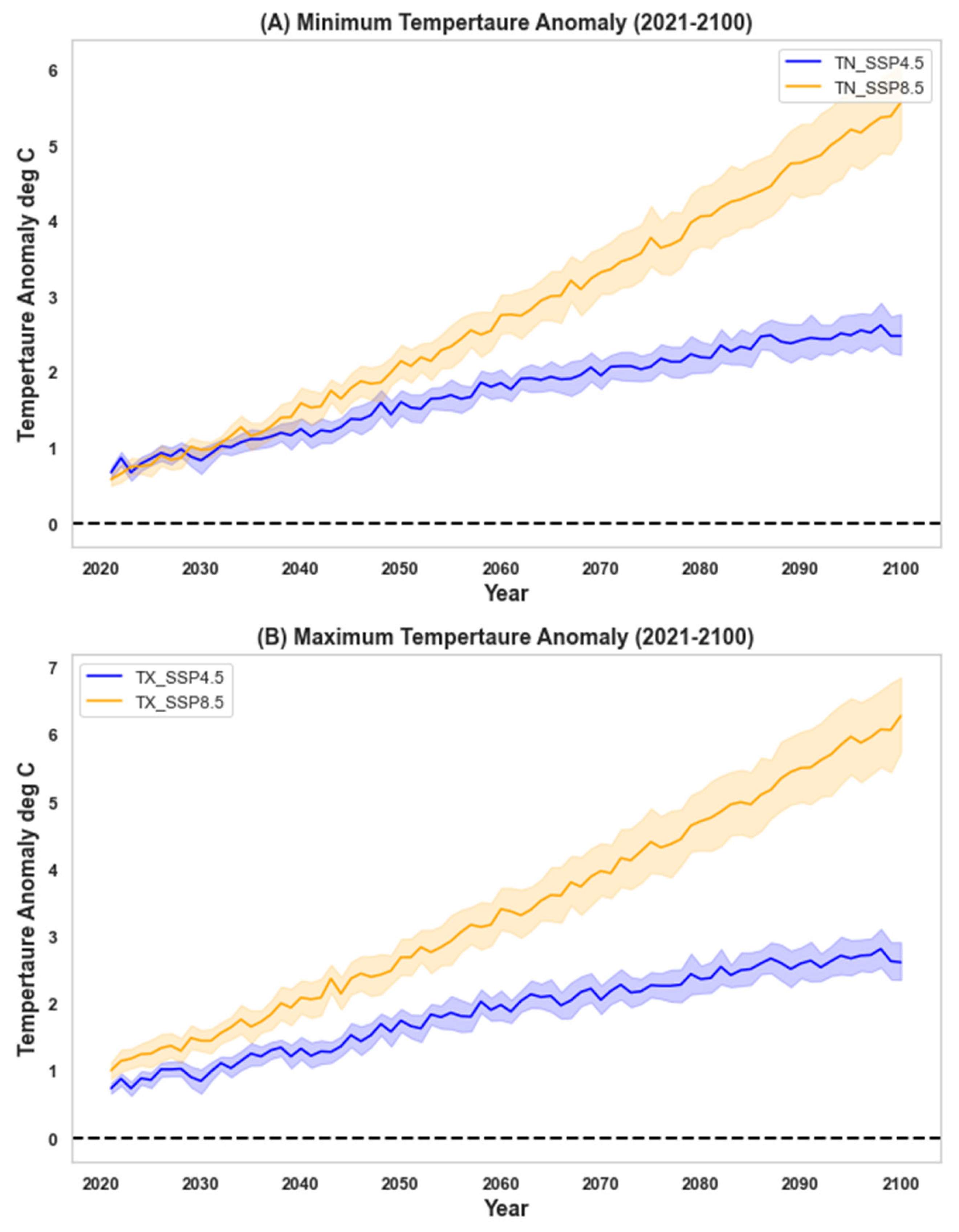
Figure 1. The anomalies of (A) minimum (TN) and (B) maximum (TX) temperatures and of (C) precipitation (Pr) for the future period (2021–2100) corresponding to the reference period (1981–2010) under the two of the Shared Socioeconomic Pathways used in this study (SSP3-4.5 and SSP5-8.5).
Atmosphere 14 01361 g001aAtmosphere 14 01361 g001b
Table 2. The general statistics of minimum (TN) and maximum (TX) temperatures and precipitation (Pr) as projected by the two different scenarios (SSP2-4.5 and SSP5-8.5) for the mid-future (2031–2060) and far-future (2061–2100) periods.
ScenarioPeriodMeanStDevSkewnessKurtosisDifferenceTrend yr−1
TNSSP2-4.52031–206012.490.29−0.03−1.282.950.03
2061–210013.390.24−0.23−1.313.850.02
SSP5-8.52031–206012.900.490.09−1.174.360.06
2061–210015.200.850.07−1.215.670.07
TXSSP2-4.52031–206018.720.29−0.02−1.330.690.03
2061–210019.610.23−0.23−1.321.570.02
SSP5-8.52031–206019.210.480.09−1.181.090.05
2061–210021.370.840.07−1.223.340.07
PrSSP2-4.52031–20602.540.020.13−0.67−1.04−0.001
2061–21002.580.02−0.441.36−1.08−0.001
SSP5-8.52031–20602.560.020.13−1.22−1.06−0.002
2061–21002.610.020.34−0.63−1.11−0.002
Table 3. Mean squared analysis of variance with treatment significance of leaf color, leaf area, plant height, total non-structure carbohydrate content (TNC), shoot reducing sugar content (RSC), proline content, and total evapotranspiration in the black calla lily.
ParametersWater Regimes
Leaf color (0–10 scale)65.1 *
Leaf area (cm2)4.11 *
Plant height (cm)2.66 *
TNC (mg g−1 dry wt.)711.0 **
RSC (mg g−1 dry wt.)92.0 **
Proline content (µg g−1 fresh wt.)1337 **
Total ET (mm d−1)5.1 **
* represents a p-value less than 0.05, and ** represents p < 0.01
Table 4. Effect of different water regimes on leaf color, leaf area, plant height, ET rate, TNC, RSC, and proline content of the black calla lily and the linear regression of different parameters vs. water regimes of the control (100%) and of 75%, 50%, and 25% of the total evapotranspiration.
ParameterWater Regimes (% of Total ET)RegressionR2
C755025
Leaf color (0–10 scale)9.4 a9.0 a7.5 b3.8 cY = 7.4 − 0.6 X0.84 **
Leaf area (cm2)21.6 a20.5 a15.6 b8.5 cY = 110.8 − 2.5 X0.88 **
Plant height (cm)22.0 a20.5 a15.6 b10.5 cY = 102.2 − 2.1 X0.90 **
ET rate (mmd−1)4.4 a4.0 a2.7 b2.2 cY = 9.7 − 0.6 X0.75 *
TNC
(mg g−1 dry wt.)
112.8 a105.6 a69.5 b55.9 cY = 102.7 − 1.6 X0.84 **
RSC
(mg g−1 dry wt.)
15.5 d16.8 a22.8 b30.2 cY = 9.8 + 0.23 X0.86 **
Proline content
(µg g−1 fresh wt.)
223.2 d240.0 a849.0 b1155.0 cY = 129.6 + 12.5 X0.91 **
* Significant at p ≤ 0.05. ** Significant at p ≤ 0.01.
Disclaimer/Publisher’s Note: The statements, opinions and data contained in all publications are solely those of the individual author(s) and contributor(s) and not of MDPI and/or the editor(s). MDPI and/or the editor(s) disclaim responsibility for any injury to people or property resulting from any ideas, methods, instructions or products referred to in the content.

