Article

Evaluation of the Performance of CMIP6 Climate Models in Simulating Rainfall over the Philippines

by
Shelly Jo Igpuara Ignacio-Reardon
1,2,3,* and
Jing-jia Luo
1,2,*
1
Institute for Climate and Application Research (ICAR)/CIC-FEMD/KLME/ILCEC, Nanjing University of Information Science and Technology, Nanjing 210044, China
2
College of Atmospheric Science, Nanjing University of Information Science and Technology, Nanjing 210044, China
3
Science and Mathematics Department, Tallahassee Community College, Tallahassee, FL 32304, USA
*
Authors to whom correspondence should be addressed.
Atmosphere 2023, 14(9), 1459; https://doi.org/10.3390/atmos14091459
Submission received: 11 August 2023 / Revised: 6 September 2023 / Accepted: 12 September 2023 / Published: 20 September 2023

Abstract

:
The Philippines is highly vulnerable to multiple climate-related hazards due to its geographical location and weak adaptation measures. Floods are the most catastrophic hazards that impact lives, livelihoods, and, consequently, the economy at large. Understanding the ability of the general circulation models to simulate the observed rainfall using the latest state-of-the-art model is essential for reliable forecasting. Based on this background, this paper objectively aims at assessing and ranking the capabilities of the recent Coupled Model Intercomparison Project Phase 6 (CMIP6) models in simulating the observed rainfall over the Philippines. The Global Precipitation Climatology Project (GPCP) v2.3 was used as a proxy to gauge the performance of 11 CMIP6 models in simulating the annual and rainy-season rainfall during 1980–2014. Several statistical metrics (mean, standard deviation, normalized root means square error, percentage bias, Pearson correlation coefficient, Mann–Kendall test, Theil–Sen slope estimator, and skill score) and geospatial measures were assessed. The results show that that CMIP6 historical simulations exhibit satisfactory effectiveness in simulating the annual cycle, though some models display wet/dry biases. The CMIP6 models generally underestimate rainfall on the land but overestimate it over the ocean. The trend analysis shows that rainfall over the country is insignificantly increasing both annually and during the rainy seasons. Notably, most of the models could correctly simulate the trend sign but over/underestimate the magnitude. The CMIP6 historical rainfall simulating models significantly agree on simulating the mean annual cycle but diverge in temporal ability simulation. The performance of the models remarkably differs from one metric to another and among different time scales. Nevertheless, the models may be ranked from the best to the least best at simulating the Philippines’ rainfall in the order GFDL, NOR, ACCESS, ENS, MRI, CMCC, NESM, FIO, MIROC, CESM, TAI, and CAN. The findings of this study form a good basis for the selection of models to be used in robust future climate projection and impact studies regarding the Philippines. The climate model developers may use the documented shortcoming of these models and improve their physical parametrization for better performance in the future.

1. Introduction

Climate change has been identified to pose threat to biodiversity and livelihoods and cause the economy to become volatile in countries that depend mostly on climate-related sectors such as agriculture. Therefore, understanding the past, current, and future climate trends, variations, and changes are vital for devising ways to curb and curtail the negative impacts of climate change. Climate models are important tools in understanding anticipated future climate changes around the globe. Nevertheless, the projection skills of climate models are largely dependent on their ability to simulate the historical climate of a given location. For instance, projections of future extreme El Niño occurrence frequencies are significantly overestimated owing to the systematic biases of current state-of-the-art climate models in simulating the past climate [1].
The global general circulation models (GCMs) have evolved, and their capabilities are improving as the model development moves from one phase to another. Numerous modeling groups around the globe have aided the development of climate models. The CMIP climate group under the World Climate Research Programme (WRCP) has been producing climate simulation models under different phases [2,3]. The current one, CMIP6, is different from the other phases in terms of the reference year and radiative forcing and the projections are grouped into four categories termed socioeconomic pathways (SSP) [4].
Several studies have evaluated the effectiveness of CMIP6 climate models in simulating different climate variables over various parts of the globe. For instance, Oduro et al. (2021) [5] assessed the mean surface temperature over Ghana and documented the better performance of the current CMIP6 models in simulating interannual variability than seasonal variability. Kim et al. (2020) [6] evaluated the teleconnection patterns responsible for heatwaves over Korea and found that the CMIP6 models skillfully simulate the heatwaves and teleconnection patterns better than the models from their predecessor (CMIP5). On the same note, Khadka et al. (2022) [7] compared the performance of CMIP6 and CMIP5 and found that the CMIP6 models could more skillfully simulate the onset, cessation, and rainy-season rain lengths than the CMIP5 models over the South Asia domain. This improved performance was attributed to the enhanced climate modelers’ skills in simulating land–atmosphere interactions [2].
Over China, Wang et al. (2021) [8] documented that some CMIP6 models exhibited dry bias during summer, whereas others showed wet bias during spring. Nevertheless, the models exhibited satisfactory skill in simulating the decadal characteristics of annual rainfall. Similar findings were documented by Ngoma et al. (2021) [9] over Uganda; some CMIP6 historical climate models overestimated/underestimated the annual rainfall cycle over the country, whereas over Nigeria, the models exhibited wet/dry bias in simulating the observed spatial and seasonal amounts of rainfall [10]. Fan et al. (2022) [11] observed that most of the CMIP6 models evaluated over the Pan-Third Pole (PTP) region can proficiently capture the observed spatiotemporal variability of mean and extreme temperature despite inherent dry bias over the Tibetan Plateau.
The Philippines has a mixed-type economy whereby 41% of the land mass is occupied by agriculture. Notably, the country is disaster-prone and is ranked among the top 10 countries (including Myanmar, Vietnam, and Thailand) that have been greatly affected by the negative impacts of climate change during 1997–2016 according to a report by Thomas et al., 2013 [12]. Additionally, the temperature has been rising over recent decades and the warming trend is expected to continue in the future [13]. The Philippines is among five countries around the globe that are projected to be negatively impacted by global warming [14]. This calls for the need for credible future rainfall projections to help devise appropriate mitigation measures to curb and mitigate the impacts of extreme events.
The frequency and intensity of extreme climate events (tropical cyclones, floods, drought, and landslides) are increasing and predicted to intensify in the future [15,16]. Climate change has aggravated these events and climate models that can accurately predict their occurrence are desperately needed to save lives and the Philippines economy at large. Nevertheless, few climate studies have been conducted on the southeast Asia region despite it being identified as one of the regions that is highly susceptible to the negative impacts of climate change.
There is a paucity of comprehensive knowledge about the performance of the current state-of-art climate models in simulating rainfall over the Philippines. For instance, Iqbal et al. (2021) [17] reported that the CMIP6 climate models could reasonably capture the observed spatiotemporal rainfall patterns over the South Asia region but that the performance of the models differs from one location to the other. This calls for the evaluation of climate models specifically tailored for each country and each climate variable. Based on this backdrop, this study objectively aims at ranking 11 CMIP6 models’ historical simulations based on their ability to reproduce the observed rainfall over the Philippines. The reliability of future climate projections is contingent on the effectiveness of the CMIP6 models to simulate the historical climate.
The rest of this paper will be structured as follows: Section 2 will elucidate the data types, the climate characteristics of the study region, and the evaluation techniques deployed. Section 3 will elaborate on the results. The discussion and conclusion will be drawn in Section 4 and Section 5.

2. Materials and Methods

2.1. Study Area

The study area is bounded by latitudes 5°–23° N and longitudes 115°–130° E, as depicted in Figure 1, and is herein referred to as the Philippine domain. The country is characterized by complex topography that ranges from the lowlands to the highest mountain heights of Mt. Apo National Park in Mindanao. The monsoons primarily drive rainfall patterns over Asia. The major monsoon systems include the summer monsoons that occur from mid–late May and extend all the way to September. The summer monsoons are normally termed “Habagat” and the winter monsoons are referred to as “Amihan” [18]. During October to November, the country normally receives some showers that result from retreating monsoons that shift to become winter monsoons. During summer monsoons southwest winds dominate, whereas during the winter monsoon season the prevailing winds shift to become northeasterly and bring cold dry conditions over the country [19]. Winter monsoons originate from Siberia/Mongolia/the South China Sea and are conveyed by the anticyclonic flow to the country. The rainfall-modulating factors over the country include tropical cyclones that originate from the mid-Pacific Ocean, monsoons systems, El Niño southern oscillation (ENSO), and mesoscale systems [20].

2.2. Data Source

The simulated monthly rainfall data from 11 CMIP6 climate models were evaluated against the observed rainfall over the Philippines from 1980–2014. The CMIP6 climate models are publicly available and archived at https://esgf-node.llnl.gov/search/cmip6/ (accessed on 17 December 2022). The CMIP6 models have different historical runs; for the sake of comparison, the first ensemble member (r1i1p1f1) of each model was used. Remarkably, the use of different ensemble members in the analysis showed no significant difference between rainfall amounts simulated by the CMIP6 models over North Africa [21]. The CMIP6 models have different horizontal scales, so all the models’ outputs were re-gridded using the bilinear interpolation method to a common horizontal resolution of 1° × 1°. Notably, the ensemble model (ENS) will be alphabetically represented by “E”. More details of the CMIP6 climate models used in this study are shown in Table 1.
The Global Precipitation and Climatology Project (GPCP), which is a gauge-based gridded dataset, was used to evaluate the capability of the models to simulate the rainfall amount, seasonality, and interannual variability of rainfall over the Philippines. The datasets are produced for monthly, pentad (five-yearly), and daily precipitation intervals from surface and satellite measurement from 1979–present (or 1997–present for daily). The World Data Center for Meteorology serves as a secondary conduit for this data in conjunction with NASA/GSFC. The GPCP One-Degree Daily Precipitation (1DD) Datasets provide daily, global 1X1-deg gridded fields of precipitation totals for October 1996–present with a delay of about three months. Moreover, the 1DD datasets draw upon several different data sources covering different areas of the globe. The complete record has been made as homogeneous as possible given the different available input sources. The satellite gauge and associated precipitation error estimates are the GPCP’s two primary monthly sources. The version 2.3 monthly product covers January 1979–present, with a delay of two to three months for data reception and processing. In addition, version 2.3, which was employed in the current study, supersedes all previous versions of the GPCP monthly product, including versions 1, 1b, V2x79, 2, 2.2, and 2.1. It should be noted that the previous versions are currently not available from the NOAA/NCEI archive.

2.3. Evaluation Metrics

This study adopted various statistical and geospatial measures. The descriptive and inferential statistics measures used included the temporal mean, Pearson correlation, percentage/relative bias, and normalized root mean square error (nRMSE). The effectiveness of the models was assessed based on their ability to simulate the movements of the Intertropical Convergence Zone (ITCZ), seasonal rainfall amounts, interannual variability, and multi-decadal trends.
This study used the normalized nRMSE to elucidate the relative average oddness of the GCM models from the reference dataset. This method is better than the use of RMSE, since it evaluates the models from the common ground by diving their RMSE, which is a statistically based formula for calculating the standard deviation (Equation (1)) by the mean/standard deviation of the reference data (Equation (2)). In this study, the RMSE was normalized by the mean, where μobs refers to the mean of the observation and is thus considered as a coefficient of variation (Equation (2)).
R M S E = 1 n 1 i = n n x i μ 2 n
n R M S E = R M S E μ o b s
Relative and percentage bias measures were used to understand the inconsistency among the CMIP6 models in simulating the observed rainfall amounts. The relative bias was divided by the observed mean field to scale all the models and evaluate them on common ground (Equation (3)). The percentage bias can be mathematically expressed as
P e r c e n t a g e   B i a s = C M I P 6 r a i n s O b s e r v r a i n s O b s e r v r a i n s 100 %
Rainfed agriculture plays a pivotal role in the economy of the Philippines, hence understanding rainfall trends is paramount. In this regard, non-parametric trend detection with a modified Mann–Kendall test was deployed [22,23]. This test signifies the sign of the trend, whereas its magnitude was tested using a non-parametric Theil–Sen slope estimator TSSE [24]. Notably, the use of non-parametric methods has been identified to be more vigorous than the use of their counterparts’ (parametric methods). This is because non-parametric methods are less susceptible to outliers/extreme values that may be present in the data [25]. These methods have been successfully used in previous studies around the globe to understand rainfall trends and magnitudes [26,27].
To accomplish the main objective of this study (ranking the models), skill scores (SS) were used following a study by Fu et al. (2013) [28]. This method combines the skills of the CMIP6 rainfall models at both the seasonal and annual scales. Since different metrics were used, the absolute error of each model in terms of individual metrics is obtained and then they are added up. For instance, in the case of the correlation coefficient, an ideal value (1) is used to capture the nonconformity. Notably, the smaller the SS, the higher the skills of the model in capturing the concerned measures and vice versa.
This study used these scalar metrics to rank the CMIP6 models: the Pearson correlation coefficient (PCC), normalized RMSE (nRMSE), absolute errors in a modified Mann–Kendal (MMK), Theil–Sen Slope Estimator (TSSE), and relative bias. Mathematically, SS can be illustrated as
S S = 1 C C + n R M S E + R . B + M M K + | T S S E |

3. Results

3.1. Annual Rainfall Cycle

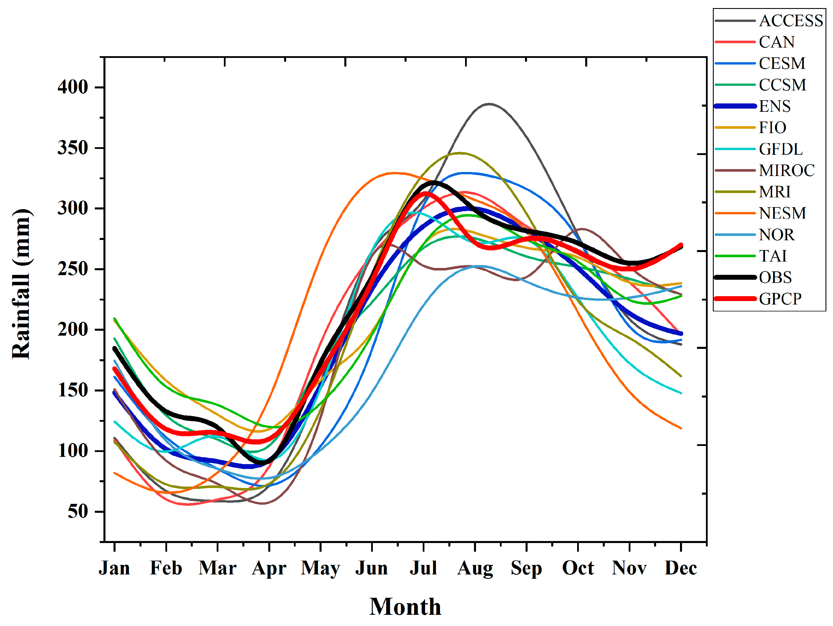
The ability of the CMIP6 models to simulate the observed annual rainfall cycle is crucial for agricultural purposes, which are season dependent. According to Sperber and Palmer (1996) [29], a good GCM should skillfully simulate the annual cycle of a given climate variable. The Philippines usually receives one rainy season as a result of monsoonal influence. Based on the observed data, the rainy season usually starts in May and persists until November (MJJASON), with a peak in mid-June (Figure 2).
The CMIP6 climate models simulate the observed annual cycle of rainfall effectively, though some models over/underestimated the observed magnitude (Figure 2). Specifically, six models (CMCC, FIO, GFDL, MIROC, NOR, and TAI) and the multi-model ensemble mean model (ENS) underestimated summer rains, whereas four models (ACCESS, CESM, MRI, and NESM) exhibited a wet bias (Figure 2). Notably, most of the models were unable to simulate the rain peak except for GFDL and FIO. This observed bias necessitates the need to correct the errors, since they are likely to be carried forward to the projections (SSPs) and create high uncertainty in them. Notably, the GPCP data show a close pattern to the observed station data and are hence deemed suitable to be used in the subsequent analysis.
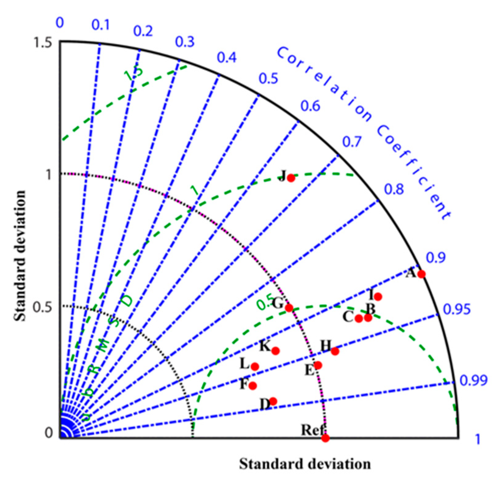
Multiple aspects of the CMIP6 models’ performances in simulating rainfall were assessed and summarized in a Taylor diagram. The results show that the models are skillful in simulating the observed annual cycle, as evidenced by the low spatial variability and the high level of consensus among the models. The best-performing model in this category is CMCC, followed by the multi-model ensemble mean (ENS), whereas the worst-performing model is NESM (Figure 3).

3.2. Latitudinal Spatial Rainfall Distribution (Hovmöller Diagram)

The seasonality of the rainfall over the Philippines is modulated by the movement of the monsoonal systems and the Intertropical Convergence Zone. The GCM has been shown to have the ability to simulate large-scale features more reliably than local features. Additionally, the effectiveness of GCMs for reliably predicting the future climate depend on their ability to capture regional historical teleconnection patterns that modulate rainfall over the area of interest [30]. The ability of the CMIP6 models to effectively simulate the movement of the ITCZ illustrates their ability to simulate teleconnection patterns that influence rainfall patterns over the study domain.
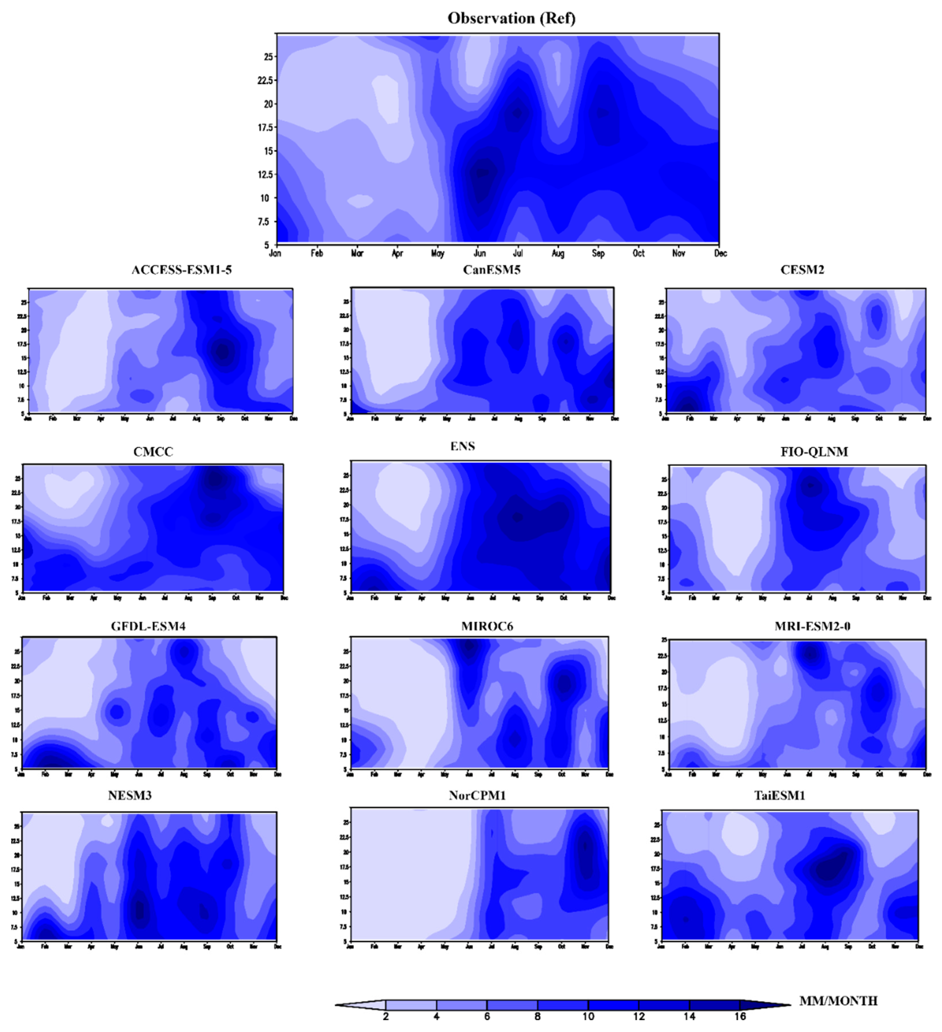
There are numerous parameters (top-cloud height, surface pressure, longwave radiation, and rainfall) that can be used to trace the movement of the ITCZ [31]. Nevertheless, these proxies seldom align; in this study, rainfall was used to trace the migration of the ITCZ. The latitudinal averages of observed rainfall over the Philippines (5°–23° N) show that the country experiences one rainy season (basically summer monsoon) and one dry season (Figure 4). Based on the observations, the rains start synchronously all over the country around mid-May and have a peak in July (Figure 4).
The models show reasonable skills in simulating the rainy-season rains season (May–November) and the dry season (February–May) (Figure 4). Notably, the CMCC simulates rainfall throughout the year at low latitudes but shows a dry condition within a latitude of 15–25° N over the region. The NorCPMI synchronously simulates the driest season during Jan–May all over the country (Figure 4). Remarkably, there is a lack of consistency amongst the CMIP6 models in simulating the onset, peak, and cessation of the rainy season (Figure 4). However, the CMIP6 models could simulate the length of the rainy-season rainfall season close to the reference dataset. These findings are concurrent with a previous study on the ability of the CMIP6 models for simulating rainy-season rains [7].
The documented discrepancies are due to a lack of skills in CMIP6 historical models for simulating the mechanisms that control rainfall over the study domain. For instance, the inability of the CMIP6 models to successfully simulate the movement of the ITCZ has been linked to the documented bias in simulating the seasonal winds over/near the tropical oceans [32]. Therefore, climate modelers are called upon to doublecheck the internal model physics of the models since they discern the model’s capability.

3.3. Spatial Distribution of Rainy-Season Rains and Related Biases in CMIP6

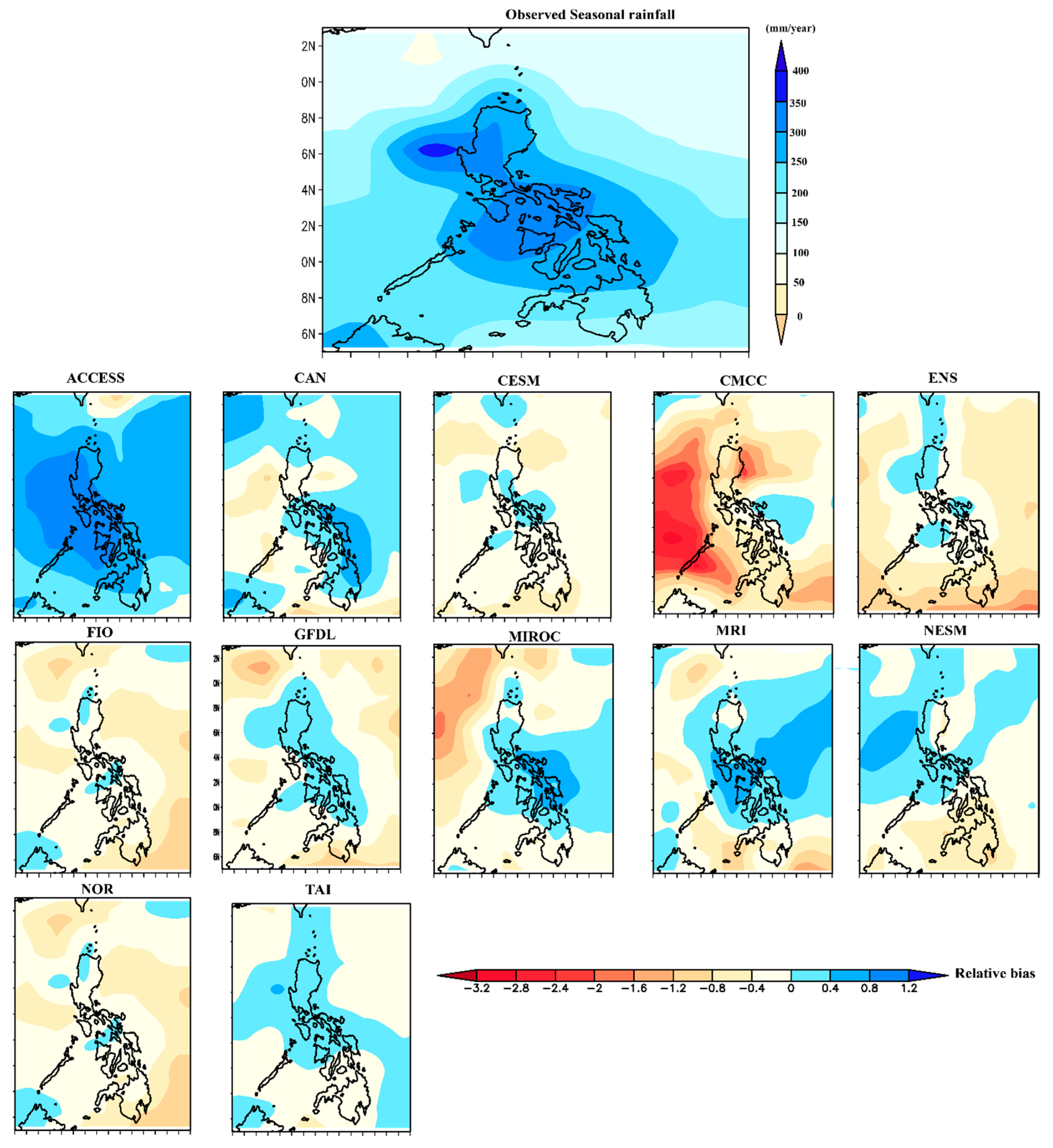
The spatial distribution of rainy-season rains shows that the northwest parts of the country receive the highest rainfall followed by the Visayas in the central region, whereas the southeast region receives the lowest amount of rainfall (Figure 5). This is attributed to the influence of topographical relief features that modulate the rainfall amount and distribution. For instance, as the southwest monsoon winds transport moisture from the Indian Ocean and the South China Sea before they reach the Philippines, the presence of high mountains such the Cordillera Mountain Range lifts the air and produces precipitation over the northern side of the country, leaving the lee side of the mountain with dry conditions.
The ability of the CMIP6 models to simulate the observed rainfall distribution is evaluated using relative bias. The results show that most of the models exhibit a dry bias over the land and a wet bias over the oceans (Figure 5). Based on the relative bias gauging metric, the driest model is CMCC whereas the wettest model is ACCESS (Figure 5). The extent of the relative bias ranged from −3.2 to 1.2 mm day−1. This necessitates the importance of improved parametrization of the CMIP6 climate models to enable them to effectively simulate the topographical features reasonably as they modulate the rainfall distribution over the Philippine highlands and around the globe.

3.4. Descriptive Statistics of the Observed Rainy-Season Rainfall and CMIP6 Models’ Simulations

The ability of the CMIP6 models to simulate the summer mean rainfall characteristics is evaluated in this subsection. The results show that most of the models depict negative bias in simulating the amount of mean summer rainfall (Table 2). Based on the models’ abilities to simulate the mean rainfall amounts, the wettest model in this category is ACCESS, with a bias of 13.1%, whereas NOR is the driest bias model among the evaluated CMIP6 models, exhibiting an understating of −15.7% compared with the reference dataset.
Notably, the South Asian region is characterized by high GCM bias in climate simulation, particularly for rainfall during the southwest summer monsoons as compared with the rest of the world [33,34]. This can be linked to the Southern Hemisphere albedo error [35]. This error arises due to the high absorption of short-wave radiation over the oceans in the Global South that leads to prominent biases in rainfall, wind, and sea surface temperatures [36,37]. Therefore, enhancing the simulation of spatial and seasonal features is likely to improve observation and model consistency in both historical simulations and future projections.
The summer rainfall amount insignificantly increased at a rate of 0.16 mm per annum during 1980–2014 (Table 2). The CMIP6 models exhibit reasonable skill in simulating the observed temporal trend, with the majority of the models simulating the correct sign of the trend but either underestimating or overestimating the magnitude. In this case, CAN overestimates the magnitude of the trend, whereas CESM, CMCC, MRI, and NESM produce the wrong sign (negative) for the trend of monsoonal summer rains over the Philippines (Table 2). This shortcomings of these CMIP6 models may be associated with the strong global interannual variability of rainfall [38]. Additionally, only two CMIP6 models (ACCESS and CAN) show credible temporal agreement with the observed interannual variability of the rainy-season rainfall.

3.5. Spatial Dissemination of Annual Rainfall and Associated CMIP6 Relative Biases

On the annual scale, the country observes a similar spatial distribution pattern of annual rainfall as the rainy-season rains. The southwest region observes the highest rainfall amounts annually compared with the rest of the country (Figure 6). The CMIP6 models display reasonable effectiveness for simulating the observed annual rainfall over the land but exhibit considerable bias over the seas. Most of the models exhibit a high bias over the ocean than over the land. The CMIP6 climate models inherent a biases range from −1.6 to 0.8 mm day−1 over the land. Notably, the driest bias of −3 mm day−1 is documented by ACCESS over the South China Sea. The multi-model ensemble documents a wet bias (0–40%) over most parts of the Philippines’ landmass, except for the southern parts of the country.

3.6. Mean Statistical Features of the CMIP6 Climate Models in Comparison with the Observed Annual Rainfall

The trend analysis shows that annual rainfall is insignificantly increasing over the Philippines at a rate of 0.2 mm yr−1 (Table 3). Notably, most of the models can capture the sign of the trend correctly, except for FIO, MIROC, NESM, and NOR, which show a negative trend in this category. All the models underestimated the magnitude of the observed annual rainfall except CAN, which had a magnitude of 0.69 mm yr−1; the observed magnitude was 0.53 mm yr−1.
The degree of spread among the evaluated CMIP6 models was assessed through standard deviation and nRMSE. NOR shows a small nRMSE (least deviation from the observation), whereas CAN has the highest nRMSE (largest deviation from the reference dataset). This depicts the existence of intermodal divergence in the CMIP6 models as compared to the observations (Table 3).
Notably, most of the models underestimate the observed annual mean rainfall in reference to the gridded dataset used in this study. Based on the mean statistics, the driest model is ACCESS, whereas the wettest model is CAN (Table 3). This dry bias may be linked to the inadequacy of GCMs to reasonably simulate the cold Arabian Sea surface temperature (SST) biases [39,40], leading to underestimation of observed summer rains over the Philippines by the CMIPs. Empirically, cold Arabian SSTs usually lead to the late onset of Asian summer rains and subsequently reduce the amount of rain according to Levine and Turner, (2012) [41].

3.7. Gauging the Multiple Skills of CMIP6 Models in Simulating Observed Monsoonal Summer Rainfall over the Philippines

Skillfully simulating the interseasonal rainfall variability is essential for the economy of the Philippines, which is highly dependent on rainfed agriculture. Additionally, the country is highly susceptible to extreme climate events, hence effectively simulating the observed rainfall characteristics is crucial for mitigating future extreme weather events. The CMIP6 models exhibit high model discordance, as they are spread apart in the Taylor diagram (Figure 7). This indicates less agreement in simulating the summer rains over the Philippines. Additionally, only a few CMIP6 models (FIO, NOR, TAI, and the multi-model ensemble) could reasonably simulate the amplitude of the rainy-season rains over the country (Figure 7), whereas other models exhibit high spatial variability, as evidenced by a standard deviation of greater than one. In this case, the least performing CMIP6 models based on the combined statistics, as depicted by the Taylor summarizing tool, are CESM and CMCC.
Remarkably, based on this category, the multi-modal ensemble (ENS) model outperforms the individual models, and it is hence considered to be the best-performing model as per this model ranking criterion. Similar findings have been recorded about the capability of the CMIP6 ENS model though using a different set of CMIP6 models [21]. This conclusion about the performance of the CMIPs ENS can be attributed to the fact that the ENS minimizes the noise in the models despite the advocation of “one model one vote”.

3.8. Taylor Diagram of CMIP6 Models Skills in Simulating Observed Annual Rainfall

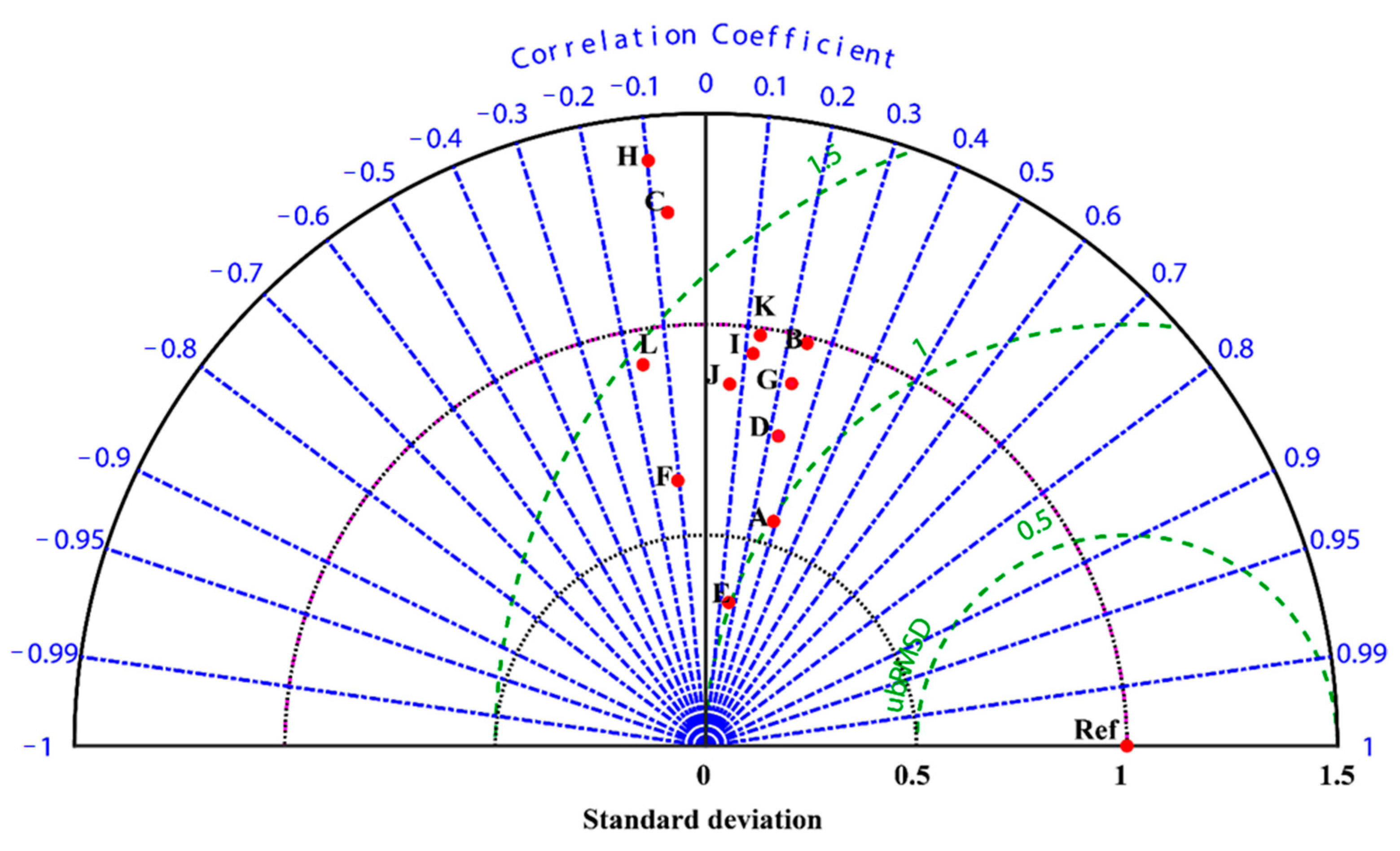
To summarize different facets of the relationship between the observed annual rainfall as documented by the GPCP and CMIP6 models, a Taylor diagram was used. The statistical intuitive metrics address the spatial pattern, the amplitude, and the RMSE. The RMSE is depicted by the green concentric semi-cycle, whereas the grey radial coordinates indicate the magnitude of the standard deviation (Figure 8). The results show that there is a lack of consensus among the CMIP6 models in terms of rainfall as they have spread apart (Figure 8). Nevertheless, most of the CMIP6 models reasonably simulate the amplitude of the observed patterns but with low spatial variability. The CESM, CMCC, and MRI models overestimated the differences between dry and wet months over the country (Figure 8). MRI showed the least ability for simulating the interannual variability of the annual rainfall. Notably, the ENS model, as represented by the alphabet (E), outperforms all the individual models (Figure 8).

3.9. Skill Score Ranking of CMIP6 over the Philippines

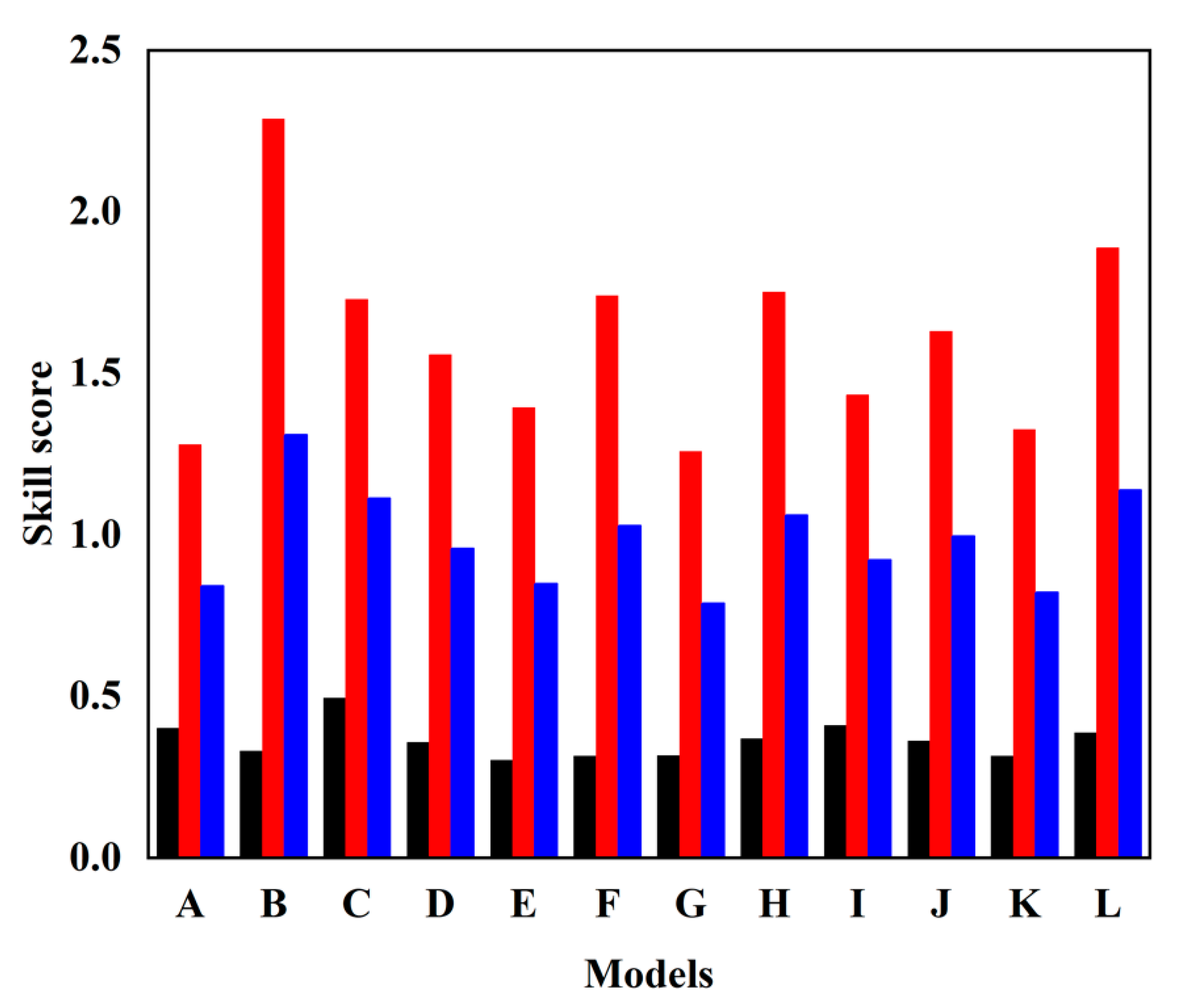
Rating the skills of the GCMs in simulating the observed climate characteristics of a given area is essential for reliable future climate projections. The credibility of GCMs projections is contingent on the capability of the GCMs to reproduce the past climate. In this regard, the performance of the CMIP6 group of models was gauged using different spatial and statistical metrics. Three different metrics were used (monsoonal summer rainfall, annual rainfall amount, and the average of the two). The results show that different models perform differently under certain measures and the performance of models differs in different time scales. For instance, the ENS outperforms all the individual models at the seasonal scale but ranks fourth out of the 11 individual CMIP6 models assessed at both the annual scale and in the overall ranking of the models. On the annual scale, the best-performing model is GFDL, whereas the worst-performing model is CAN (Figure 9).
In the final ranking, the considered CMIP6 models may be listed from the best to worst in term of simulating the observed rainfall patterns over the Philippines in the order: GFDL, NOR, ACCESS, ENS, MRI, CMCC, NESM, FIO, MIROC, CESM, TAI, and CAN. Notably, the choice of the model to be used in the projection should be based on the sole purpose of the use of the model, since different models perform differently at various time scales. Remarkably, there is not an absolutely bad model, since their skills differ in capturing certain atmospheric phenomena that modulate rainfall as the climate is governed by complex processes.

4. Discussion

The present study assessed and ranked the capability of the recent Coupled Model Intercomparison Project Phase 6 (CMIP6) models for simulating the observed rainfall over the Philippines. This was achieved by comparing the GCMs with observational datasets obtained from the Global Precipitation Climatology Project (GPCP) v2.3. The assessment was conducted in terms of spatial patterns and temporal variability for the period 1981–2014, reflecting the long-term climatology as widely advocated by the World Meteorology Organization, which defines a mean climate to be a long-term period of about thirty years. This study employed robust scalar metrics to rank the CMIP6 models; the metrics included the Pearson correlation coefficient (PCC), normalized RMSE (nRMSE), absolute errors in a modified Mann–Kendal test, Theil–Sen Slope Estimator, statistical analysis, and relative bias. The analysis was mainly based on all the models and the MME was derived by computing the simple arithmetic mean of the individual models for any rainy season from May to November.
Our results show that the CMIP6’s historical simulations exhibit satisfactory skill in simulating the annual cycle, though some models display wet/dry biases (Figure 2 and Figure 3). However, most of the models exhibit a dry bias over the land and a wet bias over the oceans (Figure 5). The dry bias over land can be linked to the inability of the CMIP6 climate models to simulate orographic effects that play a key role in modulating the rainy-season rains. The inadequacy of the CMIP models to simulate topographical relief features was observed in CMIP6’s predecessors and even regional downscaled models around the globe [26,27,42,43,44]. The Philippines is a complex archipelagic country with varied, partly mountainous topography. The effects of these important features on the climate of the country are unlikely to be well represented by GCMs. Multi-model dynamically downscaled models could therefore be useful in the analysis of local climate, so as to address the challenges of the coarse resolution of GCMs, which cannot capture the convective processes as a result of complex geomorphology. However, the main challenge of generating climate models using dynamically downscaling techniques is that they are very computationally expensive, especially when running high-resolution climate models such as the HigResMIP historical runs with at least 50 km of atmospheric resolution and 0.25° of oceanic resolution [45]. The HighResMIP experiments offer the opportunity to better understand precipitation fluctuation based on global high-resolution simulation models. Eventually, the hydrological cycle can be better reproduced to mitigate the impacts of precipitation variability on human life and the environment.
Further analysis for annual simulation showed greater bias over the ocean than over the land (Figure 6). The observed substantial dry/wet bias over the ocean/seas may be attributed to the inadequacy of CMIP6 models to effectively simulate the enormous convective activities over the South China Sea and the Indian Ocean. A similar inadequacy to simulate convective rainfall was linked to the poor parameterization of convective schemes in CMIP5 [46]. This claim is supported by Ma et al. [43], who observed that, on the tropospheric column of GCMs, there is huge warming in regions that record downward air motions based on the observations but regions that have enormous updraft activities exhibit slow warming both under greenhouse gas forcing and unified SST intensification experiments [43].
Despite the robust findings of this study, various limitations are noted that influence the current results. Examples include the limited number of models evaluated (i.e., eleven models from CMIP6), the statistical approaches employed, and the restricted number of seasons considered. Nevertheless, the results point to some remarkable findings and future directions. The study identified models that perform robustly over the region that can be used to build an ensemble for future projections. Future studies may consider resolving persistent wet biases noted over the study region. Persistent uncertainty causes various stakeholders such as policymakers and users of climate information to remain in a state of confusion about the future climate during the wet season, since the models’ reliability cannot be wholly trusted. This calls for further investigation and attribution studies into the sources of unyielding systematic biases. The overall performance in the CMIP6 models over the Philippines region calls for the model developers to improve their physical parametrization for better performance in the future.

5. Conclusions

The effectiveness of 11 CMIP6 climate models was assessed for simulating the monsoonal summer rains and annual characteristics of rainfall over the archipelagoes of the Philippines. The gridded dataset from GPCP was used as the reference data in this study. Several geostatistical and statistical metrics such as mean, nRMSE, percentage and relative bias, and skill score were used as the gauging scales. The results show that the country is characterized by a unimodal rainfall regime, termed rainy-season (summer monsoon) rains, with one dry season (winter monsoon). The spatial distribution of both the annual and summer rains shows higher rainfall amounts on the southeastern side of the country. Trend analysis from 1980–2014 shows that the observed rainfall amounts during the summer and annually are increasing insignificantly throughout the country at a rate of 0.16 mm yr−1 and 0.2 mm yr−1, respectively. This can be linked to an increase in greenhouse gases in the atmosphere leading to high convective activity over the land and ocean.
The CMIP6 models show satisfactory effectiveness for simulating the observed summer rainfall over the country, though some models underestimate the monthly amounts within the season. The majority of the models exhibit dry biases over the ocean but show wet biases over the land ocean. Notably, the wettest bias was recorded by ACCESS over the South China Sea. The CMIP6 exhibits unsatisfactory ability for simulating interannual variability, which was characterized by huge divergence among the models. The ENS outperformed the evaluated individual CMIP6 models in simulating summer rains over the Philippines. Remarkably, most of the CMIP6 models could simulate the observed rainfall trends, though they over/underestimated the magnitude of them. Notably, the performance of the models was different at different time scales and under various evaluation metrics. Nevertheless, considering all the evaluation measures and the time scale, this study attempts to rank the evaluated CMIP6 models from the best to worst as GFDL, NOR, ACCESS, ENS, MRI, CMCC, NESM, FIO, MIROC, CESM, TAI, and CAN. Therefore, the selection of the CMIP6 model to be used in future climate projections should be based on the intended use of the model.
The findings of this study are useful in identifying the models that may be used to produce reliable projections of the future climate under different SSPs scenarios. The climate model developers may use the CMIP6 models’ shortcomings that have been identified in this study to improve the model parametrization for better performance in the future. Caution should be exercised when choosing the model to be used in future projections due to the documented differential performance at various time scales of the CMIP6 models. The choice of the model should be based solely on the intended use of the model. Climate scientists should incorporate bias correction when deploying CMIP6 models for impact studies and climate projections due to inherent biases.

Author Contributions

Conceptualization, S.J.I.I.-R.; methodology, S.J.I.I.-R.; software S.J.I.I.-R.; validation, S.J.I.I.-R.; formal analysis, S.J.I.I.-R.; investigation, S.J.I.I.-R.; resources, S.J.I.I.-R. and J.-j.L.; data curation, S.J.I.I.-R.; writing—original draft preparation, S.J.I.I.-R.; writing—review and editing, S.J.I.I.-R. and J.-j.L.; visualization, S.J.I.I.-R.; supervision, J.-j.L.; project administration, J.-j.L.; funding acquisition, J.-j.L. All authors have read and agreed to the published version of the manuscript.

Funding

This work is supported by the National Natural Science Foundation of China (Grant 42088101 and 42030605).

Institutional Review Board Statement

Not applicable.

Informed Consent Statement

Not applicable.

Data Availability Statement

Not applicable.

Acknowledgments

The authors are thankful to Nanjing University of Information Science and Technology (NUIST), China for offering research atmosphere and technical support. Additionally, we are thankful to the WRCP for making available the CMIP6 data and GPCP group. We are also grateful to the Philippine Atmospheric, Geophysical, and Astronomical Services Administration-Department of Science and Technology (PAGASA-DOST) for allowing access to the observation data. We remain grateful to the editor and the reviewers for their constructive critiques.

Conflicts of Interest

The authors declare no conflict of interest.

References

  1. Tang, T.; Luo, J.-J.; Peng, K.; Qi, L.; Tang, S. Over-Projected Pacific Warming and Extreme El Niño Frequency Due to CMIP5 Common Biases. Natl. Sci. Rev. 2021, 8, nwab056. [Google Scholar] [CrossRef] [PubMed]
  2. Taylor, K.E.; Stouffer, R.J.; Meehl, G.A. An Overview of CMIP5 and the Experiment Design. Bull. Am. Meteorol. Soc. 2012, 93, 485–498. [Google Scholar] [CrossRef]
  3. Eyring, V.; Bony, S.; Meehl, G.A.; Senior, C.A.; Stevens, B.; Stouffer, R.J.; Taylor, K.E. Overview of the Coupled Model Intercomparison Project Phase 6 (CMIP6) Experimental Design and Organization. Geosci. Model. Dev. 2016, 9, 1937–1958. [Google Scholar] [CrossRef]
  4. Gidden, M.J.; Riahi, K.; Smith, S.J.; Fujimori, S.; Luderer, G.; Kriegler, E.; van Vuuren, D.P.; van den Berg, M.; Feng, L.; Klein, D.; et al. Global Emissions Pathways under Different Socioeconomic Scenarios for Use in CMIP6: A Dataset of Harmonized Emissions Trajectories through the End of the Century. Geosci. Model. Dev. 2019, 12, 1443–1475. [Google Scholar] [CrossRef]
  5. Oduro, C.; Shuoben, B.; Ayugi, B.; Beibei, L.; Babaousmail, H.; Sarfo, I.; Ullah, S.; Ngoma, H. Observed and Coupled Model Intercomparison Project 6 Multimodel Simulated Changes in Near-surface Temperature Properties over Ghana during the 20th Century. Int. J. Climatol. 2022, 42, 3681–3701. [Google Scholar] [CrossRef]
  6. Kim, M.; Yu, D.; Oh, J.; Byun, Y.; Boo, K.; Chung, I.; Park, J.; Park, D.R.; Min, S.; Sung, H.M. Performance Evaluation of CMIP5 and CMIP6 Models on Heatwaves in Korea and Associated Teleconnection Patterns. J. Geophys. Res. Atmos. 2020, 125, e2020JD032583. [Google Scholar] [CrossRef]
  7. Khadka, D.; Babel, M.S.; Abatan, A.A.; Collins, M. An Evaluation of CMIP5 and CMIP6 Climate Models in Simulating Summer Rainfall in the Southeast Asian Monsoon Domain. Int. J. Climatol. 2022, 42, 1181–1202. [Google Scholar] [CrossRef]
  8. Wang, L.; Zhang, J.; Shu, Z.; Wang, Y.; Bao, Z.; Liu, C.; Zhou, X.; Wang, G. Evaluation of the Ability of CMIP6 Global Climate Models to Simulate Precipitation in the Yellow River Basin, China. Front. Earth Sci. 2021, 9, 751974. [Google Scholar] [CrossRef]
  9. Ngoma, H.; Wen, W.; Ayugi, B.; Babaousmail, H.; Karim, R.; Ongoma, V. Evaluation of Precipitation Simulations in CMIP6Models over Uganda. Int. J. Climatol. 2021, 41, 4743–4768. [Google Scholar] [CrossRef]
  10. Shiru, M.S.; Chung, E.S. Performance Evaluation of CMIP6 Global Climate Models for Selecting Models for Climate Projection over Nigeria. Theor. Appl. Climatol. 2021, 146, 599–615. [Google Scholar] [CrossRef]
  11. Fan, X.; Duan, Q.; Shen, C.; Wu, Y.; Xing, C. Evaluation of Historical CMIP6 Model Simulations and Future Projections of Temperature over the Pan-Third Pole Region. Environ. Sci. Pollut. Res. 2022, 29, 26214–26229. [Google Scholar] [CrossRef] [PubMed]
  12. Thomas, V.; Albert, J.R.G.; Perez, R.T. Climate-Related Disasters in Asia and the Pacific. ADB Econ. Work. Pap. Ser. 2013, 358, 20–23. [Google Scholar] [CrossRef]
  13. IPCC Climate Change 2014: Synthesis Report. Contribution of Working Groups I, II and III to the Fifth Assessment Report of the Intergovernmental Panel on Climate Change; IPCC: Geneva, Switzerland, 2014.
  14. Pour, S.H.; Wahab, A.K.A.; Shahid, S. Physical-Empirical Models for Prediction of Seasonal Rainfall Extremes of Peninsular Malaysia. Atmos. Res. 2020, 233, 104720. [Google Scholar] [CrossRef]
  15. Gariano, S.L.; Guzzetti, F. Landslides in a Changing Climate. Earth Sci. Rev. 2016, 162, 227–252. [Google Scholar] [CrossRef]
  16. Tabari, H. Climate Change Impact on Flood and Extreme Precipitation Increases with Water Availability. Sci. Rep. 2020, 10, 13768. [Google Scholar] [CrossRef]
  17. Iqbal, Z.; Shahid, S.; Ahmed, K.; Ismail, T.; Ziarh, G.F.; Chung, E.-S.; Wang, X. Evaluation of CMIP6 GCM Rainfall in Mainland Southeast Asia. Atmos. Res. 2021, 254, 105525. [Google Scholar] [CrossRef]
  18. Veloria, A.; Perez, G.J.; Tapang, G.; Comiso, J. Improved Rainfall Data in the Philippines through Concurrent Use of GPM IMERG and Ground-Based Measurements. Remote. Sens. 2021, 13, 2859. [Google Scholar] [CrossRef]
  19. Kripalani, R.H.; Kulkarni, A. Climatic Impact of El Niño/La Niña on the Indian Monsoon: A New Perspective. Weather 1997, 52, 39–46. [Google Scholar] [CrossRef]
  20. Cruz, F.T.; Narisma, G.T.; Villafuerte, M.Q.; Cheng Chua, K.U.; Olaguera, L.M. A Climatological Analysis of the Southwest Monsoon Rainfall in the Philippines. Atmos. Res. 2013, 122, 609–616. [Google Scholar] [CrossRef]
  21. Babaousmail, H.; Hou, R.; Ayugi, B.; Ojara, M.; Ngoma, H.; Karim, R.; Rajasekar, A.; Ongoma, V. Evaluation of the Performance of CMIP6 Models in Reproducing Rainfall Patterns over North Africa. Atmosphere 2021, 12, 475. [Google Scholar] [CrossRef]
  22. Mann, H.B. Nonparametric Tests Against Trend. Econometrica 1945, 13, 245. [Google Scholar] [CrossRef]
  23. Kendall, M.G. Rank Correlation Methods, 4th ed.; Griffin: London, UK, 1957. [Google Scholar]
  24. Sen, P.K. Estimates of the Regression Coefficient Based on Kendall’s Tau. J. Am. Stat. Assoc. 1968, 63, 1379–1389. [Google Scholar] [CrossRef]
  25. Xu, M.; Kang, S.; Wu, H.; Yuan, X. Detection of Spatio-Temporal Variability of Air Temperature and Precipitation Based on Long-Term Meteorological Station Observations over Tianshan Mountains, Central Asia. Atmos. Res. 2018, 203, 141–163. [Google Scholar] [CrossRef]
  26. Mumo, L.; Yu, J. Gauging the Performance of CMIP5 Historical Simulation in Reproducing Observed Gauge Rainfall over Kenya. Atmos. Res. 2020, 236, 104808. [Google Scholar] [CrossRef]
  27. Ayugi, B.; Tan, G.; Gnitou, G.T.; Ojara, M.; Ongoma, V. Historical Evaluations and Simulations of Precipitation over East Africa from Rossby Centre Regional Climate Model. Atmos. Res. 2020, 232, 104705. [Google Scholar] [CrossRef]
  28. Fu, G.; Liu, Z.; Charles, S.P.; Xu, Z.; Yao, Z. A Score-Based Method for Assessing the Performance of GCMs: A Case Study of Southeastern Australia. J. Geophys. Res. Atmos. 2013, 118, 4154–4167. [Google Scholar] [CrossRef]
  29. Turner, A.; Sperber, K.R.; Slingo, J.; Meehl, G.; Mechoso, C.R.; Kimoto, M.; Giannini, A. Modelling Monsoons: Understanding and Predicting Current and Future Behaviour. In Global Monsoon System, the Research and Forecast, 2nd ed.; World Scientific Pub Co., Ltd.: Singapore, 2011. [Google Scholar]
  30. Bhattacharjee, P.S.; Zaitchik, B.F. Perspectives on CMIP5 Model Performance in the Nile River Headwaters Regions. Int. J. Climatol. 2015, 35, 4262–4275. [Google Scholar] [CrossRef]
  31. Nicholson, S.E. The West African Sahel: A Review of Recent Studies on the Rainfall Regime and Its Interannual Variability. ISRN Meteorol. 2013, 2013, 453521. [Google Scholar] [CrossRef]
  32. Larson, S.M.; Kirtman, B.P.; Vimont, D.J. A Framework to Decompose Wind-Driven Biases in Climate Models Applied to CCSM/CESM in the Eastern Pacific. J. Clim. 2017, 30, 8763–8782. [Google Scholar] [CrossRef]
  33. Annamalai, H.; Hamilton, K.; Sperber, K.R. The South Asian Summer Monsoon and Its Relationship with ENSO in the IPCC AR4 Simulations. J. Clim. 2007, 20, 1071–1092. [Google Scholar] [CrossRef]
  34. Turner, A.G.; Annamalai, H. Climate Change and the South Asian Summer Monsoon. Nat. Clim. Chang. 2012, 2, 587–595. [Google Scholar] [CrossRef]
  35. Haywood, J.M.; Jones, A.; Dunstone, N.; Milton, S.; Vellinga, M.; Bodas-Salcedo, A.; Hawcroft, M.; Kravitz, B.; Cole, J.; Watanabe, S.; et al. The Impact of Equilibrating Hemispheric Albedos on Tropical Performance in the HadGEM2-ES Coupled Climate Model. Geophys. Res. Lett. 2016, 43, 395–403. [Google Scholar] [CrossRef]
  36. Kay, J.E.; Wall, C.; Yettella, V.; Medeiros, B.; Hannay, C.; Caldwell, P.; Bitz, C. Global Climate Impacts of Fixing the Southern Ocean Shortwave Radiation Bias in the Community Earth System Model (CESM). J. Clim. 2016, 29, 4617–4636. [Google Scholar] [CrossRef]
  37. Lauer, A.; Jones, C.; Eyring, V.; Evaldsson, M.; Hagemann, S.; Mäkelä, J.; Martin, G.; Roehrig, R.; Wang, S. Process-Level Improvements in CMIP5 Models and Their Impact on Tropical Variability, the Southern Ocean, and Monsoons. Earth Syst. Dyn. 2018, 9, 33–67. [Google Scholar] [CrossRef]
  38. Vicente-Serrano, S.; García-Herrera, R.; Peña-Angulo, D.; Tomas-Burguera, M.; Domínguez-Castro, F.; Noguera, I.; Calvo, N.; Murphy, C.; Nieto, R.; Gimeno, L.; et al. Do CMIP models capture long-term observed annual precipitation trends? Clim. Dyn. 2022, 58, 2825–2842. [Google Scholar] [CrossRef]
  39. Levine, R.C.; Turner, A.G.; Marathayil, D.; Martin, G.M. The Role of Northern Arabian Sea Surface Temperature Biases in CMIP5 Model Simulations and Future Projections of Indian Summer Monsoon Rainfall. Clim. Dyn. 2013, 41, 155–172. [Google Scholar] [CrossRef]
  40. Sandeep, S.; Ajayamohan, R.S. Origin of Cold Bias over the Arabian Sea in Climate Models. Sci. Rep. 2014, 4, 6403. [Google Scholar] [CrossRef]
  41. Levine, R.C.; Turner, A.G. Dependence of Indian Monsoon Rainfall on Moisture Fluxes across the Arabian Sea and the Impact of Coupled Model Sea Surface Temperature Biases. Clim. Dyn. 2012, 38, 2167–2190. [Google Scholar] [CrossRef]
  42. Favre, A.; Philippon, N.; Pohl, B.; Kalognomou, E.-A.; Lennard, C.; Hewitson, B.; Nikulin, G.; Dosio, A.; Panitz, H.-J.; Cerezo-Mota, R. Spatial Distribution of Precipitation Annual Cycles over South Africa in 10 CORDEX Regional Climate Model Present-Day Simulations. Clim. Dyn. 2016, 46, 1799–1818. [Google Scholar] [CrossRef]
  43. Ma, J.; Xie, S.-P.; Kosaka, Y. Mechanisms for Tropical Tropospheric Circulation Change in Response to Global Warming. J. Clim. 2012, 25, 2979–2994. [Google Scholar] [CrossRef]
  44. Raghavan, S.V.; Liu, J.; Nguyen, N.S.; Vu, M.T.; Liong, S.Y. Assessment of CMIP5 Historical Simulations of Rainfall over Southeast Asia. Theor. Appl. Climatol. 2018, 132, 989–1002. [Google Scholar] [CrossRef]
  45. Haarsma, R.J.; Roberts, M.J.; Vidale, P.L.; Senior, C.A.; Bellucci, A.; Bao, Q.; Chang, P.; Corti, S.; Fučkar, N.S.; Guemas, V.; et al. High-resolution model intercomparison project (HighResMIP v1.0) for CMIP6. Geosci. Model Dev. 2016, 9, 4185–4208. [Google Scholar] [CrossRef]
  46. Hohenegger, C.; Brockhaus, P.; Schär, C. Towards Climate Simulations at Cloud-Resolving Scales. Meteorol. Z. 2008, 17, 383–394. [Google Scholar] [CrossRef] [PubMed]
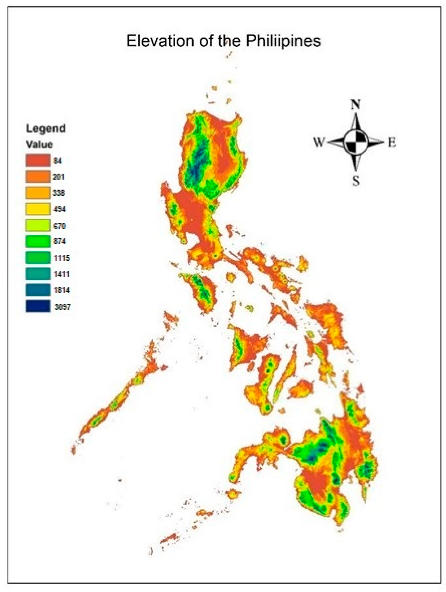
Figure 1. The geographical location of the Philippine highlands. The background color depicts the elevation of the region from the mean sea level (m).
Atmosphere 14 01459 g001
Figure 2. The annual rainfall cycle over the Philippines based on the simulations of the CMIP6 individual models and multi-model ensemble mean (thick blue color), GPCP (thick red color), and observed rainfall (thick black color).
Atmosphere 14 01459 g002
Figure 3. Taylor diagram depicting the ability of the CMIP6 models in simulating the observed annual rainfall cycle over the Philippines. The letters indicate the CMIP6 models as follows; A: ACCESS, B: CAN, C: CESM, D: CMCC, E: ENS, F: FIO, G: GFDL, H: MIROC, I: MRI, J: NESM, K: NOR, and L: TAI.
Atmosphere 14 01459 g003
Figure 4. Hovmöller diagram representing longitudinal average along 115°–130° N of monthly mean rainfall over the Philippines in mm per month.
Atmosphere 14 01459 g004
Figure 5. Spatial distribution of the rainy-season rains (mm) during May–November based on the GPCP dataset (first panel) and the corresponding bias of the CMIP6 models relative to GPCP.
Atmosphere 14 01459 g005
Figure 6. Spatial distribution of annual mean rainfall (mm) based on the GPCP dataset (first panel) and the bias of CMIP6 models relative to GPCP.
Atmosphere 14 01459 g006
Figure 7. The Taylor diagram representing the multiple statistical relationships between the observed rains and CMIP6 models during May–November. The letters stand for the CMIP6 models, i.e., A: ACCESS, B: CAN, C: CESM, D: CMCC, E: ENS, F: FIO, G: GFDL, H: MIROC, I: MRI, J: NESM, K: NOR, and L: TAI.
Atmosphere 14 01459 g007
Figure 8. Taylor diagram representing the relationship between CMIP6 models in simulating the observed annual rainfall (Ref). The letters denote the CMIP6 models: A: ACCESS, B: CAN, C: CESM, D: CMCC, E: ENS, F: FIO, G: GFDL, H: MIROC, I: MRI, J: NESM, K: NOR, and L: TAI.
Atmosphere 14 01459 g008
Figure 9. Skill score ranking of the CMIP6 models in simulating mean observed rainfall over the Philippines annually (red), during May–November (black), and overall (blue). The letters denote A: ACCESS, B: CAN, C: CESM, D: CMCC, E: ENS, F: FIO, G: GFDL, H: MIROC, I: MRI, J: NESM, K: NOR, and L: TAI.
Atmosphere 14 01459 g009
Table 1. Characteristics of the CMIP6 models used including model name, horizontal resolution, and the modeling institution.
Model
Abbreviation
Alphabet UsedHorizontal ResolutionModeling Centre
ACCESS-ESM1-5ACCESS (A)250 kmCommonwealth Scientific and Industrial Research Organization and Bureau of Meteorology, Australia
CanESM5CAN (B)500 kmCanadian Centre for Climate Modeling and Analysis (Canada)
CESM2CESM (C)100 kmNational Center for Atmospheric Research (NCAR) Boulder, CO, USA
CMCCCMCC (D)100 kmFondazione Centro Euro-Mediterraneo sui Cambiamenti Climatici, Lecce 73100, Italy
FIO-QLNMFIO (F)100 kmFirst Institute of Oceanography, State Oceanic Administration, Qingdao 266061, China), QNLM (Qingdao National Laboratory for Marine Science and Technology, Qingdao 266237, China)
GFDL-ESM4GFDL (G)100 kmNational Oceanic and Atmospheric Administration, Geophysical Fluid Dynamics Laboratory, Princeton, NJ 08540, USA
MIROC6MIROC(H)250 kmJAMSTEC (Japan Agency for Marine-Earth Science and Technology, Kanagawa, Japan), AORI (Atmosphere and Ocean Research Institute, The University of Tokyo, Chiba, Japan), and NIES (National Institute for Environmental Studies, Ibaraki, Japan
MRI-ESM2-0MRI (I)100 kmMeteorological Research Institute, Tsukuba, Ibaraki 305-0052, Japan
NESM3NESM (J)250 kmThe Nanjing University of Information Science and Technology, Nanjing, 210044, China
NorCPM1NOR (K)250 kmNorESM Climate modeling Consortium consisting of CICERO (Center for International Climate and Environmental Research, Oslo 0349), MET-Norway (Norwegian Meteorological Institute, Oslo 0313), NERSC (Nansen Environmental and Remote Sensing Center, Bergen 5006), NILU (Norwegian Institute for Air Research, Kjeller 2027), UiB (University of Bergen, Bergen 5007), UiO (University of Oslo, Oslo 0313) and UNI (Uni Research, Bergen 5008), Norway. Mailing address: NCC, c/o MET-Norway, Henrik Mohns plass 1, Oslo 0313, Norway
TaiESM1TAI (L)100 kmResearch Center for Environmental Changes, Academia Sinica, Nankang, Taipei 11529, Taiwan
Table 2. Statistical characteristics of rainfall during May–November both in observed and CMIP6 model data. The bolded numbers depict statistically significant values at p 0.1 .
ClassMeanstdevBiasRMSEnRMSEMMKTSSE
Obs268.117.3 0.160.32
ACCESS302.526.113.3%89.70.340.140.6
CAN278.118.24.1%64.10.240.280.72
CESM267.926.50.3%60.90.23−0.12−0.42
CMCC255.014.5−4.5%43.20.16−0.02−0.02
ENS261.36.2−2.2%47.30.180.150.13
FIO240.114.9−10.1%31.70.120.100.21
GFDL250.021.0−6.4%41.80.160.160.48
MIROC255.922.3−4.2%47.10.180.010.005
MRI271.519.21.6%59.60.22−0.04−0.22
NESM265.716.7−0.5%53.00.20−0.03−0.075
NOR217.119.9−15.7%25.50.100.02−0.05
TAI255.715.5−4.3%45.70.170.140.3
Table 3. The statistical characteristics of annual rainfall both in observations and the CMIP6 models. The bolded values depict statistically significant MMK values at p ≤ 0.
ClassMeanstdevBiasRMSEnRMSEMMKTSSE
Obs206.118.4 0.200.53
ACCESS174.510.3−15.3%40.70.200.110.13
CAN218.218.25.9%118.20.570.280.69
CESM195.223.4−5.3%44.90.220.030.08
CMCC206.514.40.2%49.00.240.010.05
ENS196.36.4−4.7%38.80.190.100.09
FIO189.311.7−8.1%35.30.17−0.04−0.05
GFDL186.216.3−9.6%32.20.160.060.20
MIROC188.625.7−8.5%42.10.20−0.03−0.08
MRI187.017.3−9.2%34.20.170.020.02
NESM193.715.9−6.0%39.20.19−0.06−0.07
NOR194.718.1−5.5%26.90.13−0.01−0.05
TAI211.516.92.7%56.20.270.130.21
Disclaimer/Publisher’s Note: The statements, opinions and data contained in all publications are solely those of the individual author(s) and contributor(s) and not of MDPI and/or the editor(s). MDPI and/or the editor(s) disclaim responsibility for any injury to people or property resulting from any ideas, methods, instructions or products referred to in the content.