1. Introduction
In the context of global warming, widespread blizzards and record-breaking snowstorms continue to occur with great frequency [
1,
2]. Large mid-latitude areas over the contiguous United States (CONUS), Europe, and Asia have experienced successive cold winters of severely low temperature and winter storms since the beginning of the 21st century [
3,
4,
5]. In recent years, the damage of extreme cold events increases significantly, especially in United States. For example, the cold wave of February 2021 in the United States’ Southern Plains, having strong intensity, long cold duration, and widespread disruptive snowfall [
6], caused the collapse of the Texas energy infrastructure, which was more than twice as costly as the total 2020 hurricanes in the Atlantic [
7]. Therefore, the extreme cold trend with climate change is being widely debated. Previous studies have shown that the atmosphere circulation’s variability linked to sea ice loss in the Arctic plays a key role [
8,
9,
10,
11,
12,
13,
14].
However, there is argument over the number of cold extremes reduced by global warming [
15]. Being suggested as a source region for cold extremes across the mid-latitude, the Arctic has rapidly warmed, while cold extremes have occurred less, with moderate intensity [
16,
17,
18]. But in US and Asia, the variation in the cold extremes is different. The extreme cold and heavy snowfall in 2021 and 2022 was the costliest natural disaster in the US. Therefore, the linkage between the Arctic and the cold extremes is not linear, but more complex.
The seasonal blizzard frequency has displayed a distinct upward trend, with a more substantial rise over the past two decades [
19,
20]. The outbreak of bitter cold air across southern Canada and the U.S. Midwest and East Coast in January 2019, the frigid start of 2011, and the cold weather in 2014, etc., are a few examples of strong cold waves that have striked the mid-latitude CONUS region.
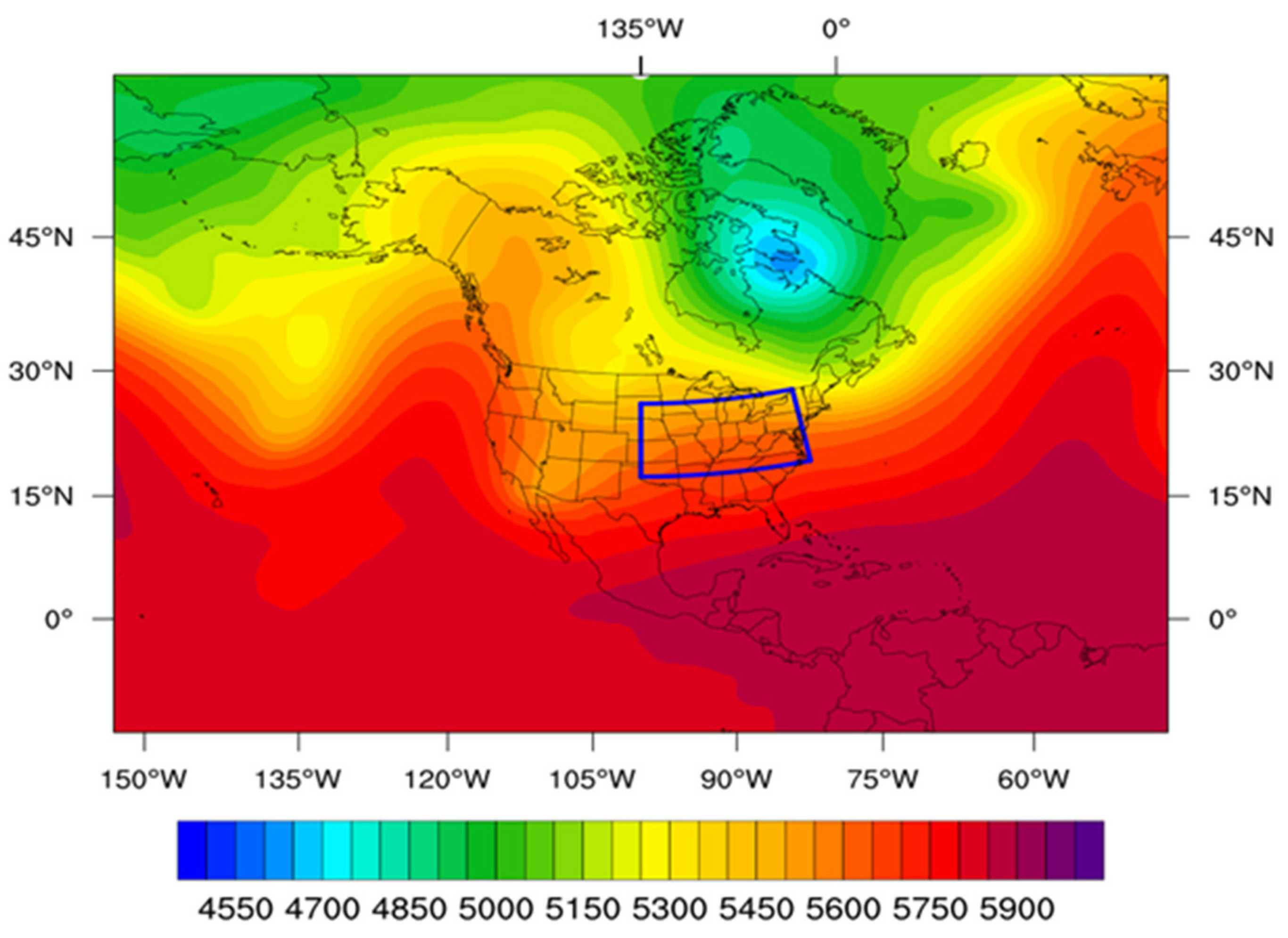
Figure 1 illustrates a typical Arctic cold air outbreak case that occurred during 31 January–2 February 2011. The storm developed when cold Arctic air pushed south, leading to heavy snow, ice, freezing rain, and frigid winds that swept across the Midwest and Eastern U.S. The blue box in
Figure 1 outlines the area of interest of the present study, which is also the area often struck by severe winter storms.
Concurrent with the increases in extreme cold winters since the 2010s, the Arctic sea ice (ASI) area has exhibited dramatic decreases with rapid temperature increases in the polar region. The paradox of global warming and successive cold winters of low temperature remains controversial and no consensus has been reached [
21,
22,
23]. The question here is the following: Is there any connection between Arctic change and cold air outbreaks in winter in eastern CONUS? Among all the possible factors that may affect winter weather over eastern CONUS, we are particularly concerned about polar vortex, a planetary-scale low pressure system that hovers over the Arctic in the winter, occupies the middle and upper troposphere and extends into the stratosphere. It is the circulation system that directly responds to Arctic surface changes and also the system that bridges the Arctic to mid- and lower-latitude regions. The transient displacements of the edge of the polar vortex accompanied by blockings are directly related to cold air outbreaks in the mid-latitudes [
24,
25]. Based on the above discussion, it is hypothesized that the polar vortex and mid-latitude blocking response to Arctic sea ice loss/warming are two important factors that contribute to increased cold winters over eastern CONUS. In this study, we will demonstrate how Arctic sea ice loss and cold winters in eastern CONUS are dynamically connected through the polar vortex.
This study will demonstrate how Arctic sea ice loss and cold winters in eastern CONUS are dynamically connected through polar vortex weakening. Specifically, we address three major issues, listed below.
Investigate the trends of Arctic sea ice and surface air temperature during the period 1980–2018. Based on the result, identify two decades with anomalous high and low extent of Arctic sea ice, respectively (hereafter high-ice and low-ice phase), for comparative study.
Reveal transient temperature variations during the above two phases, compare the occurrence frequency of cold air outbreaks over eastern CONUS between the two phases.
Explore the atmospheric response to Arctic changes with a focus on polar vortex characteristics and differences between the above two phases, build the linkage between Arctic sea ice loss and polar vortex weakening, and investigate their impacts on mid-latitude CONUS extreme cold winters.
2. Data and Methods
The ERA-Interim reanalysis dataset, which is produced by the European Centre for Medium-Range Weather Forecasts (ECMWF), is implemented in the present study. It is a global gridded dataset at approximately 0.7-degree spatial resolution with 37 atmospheric levels in the vertical. The ERA-I reanalysis dataset is selected for the present study because it is produced with the ECMWF advanced atmospheric model and assimilation system. It also includes accurate satellite remote sensing observations that have been available since 1979. This dataset is a reliable and frequently used atmospheric reanalysis dataset [
26]. In addition, the fifth-generation European Centre for Medium-Range Weather Forecasts (ERA5) [
27] are also used in the following analysis.
Monthly mean Arctic sea ice cover and surface air temperature at 2 m height above the ground level to the north of 60° N are analyzed to explore their changes and trends for the period of 1980–2018. This period is selected for two reasons: (1) satellite data have only been available since 1979, and the ERA-I incorporates satellite data and other most reliable in situ observations for this period; (2) this period is long enough to represent the climate’s state. Meanwhile, it can also reflect the most recent weather and climate conditions in response to Arctic sea ice loss. The Arctic sea ice extent usually shrinks to its minimum in September, and exerts significant impacts on the atmospheric conditions in the following winter months. For this reason, Arctic sea ice extent in September over 1980–2018 are analyzed and two distinct phases, i.e., the high-ice (1990–1999) and low-ice (2007–2016) phases, are identified for comparative study.
In order to quantify the intensity and frequency of cold air outbreaks over eastern CONUS (denoted by the blue box in
Figure 1), a coldness index is constructed in the present study based on daily surface air temperature at 2 m (hereafter T2m) above the ground level averaged over eastern CONUS. It is expressed as
where N is the total number of days during the study period,
Xi is T2m at each day,
is the average of T2m over the study period, and
STD is the standard deviation of T2m during the study period.
The coldness index actually reflects the degree of T2m deviation from its climatological mean. Larger negative index values indicate stronger old air outbreaks. Time series of daily coldness index are calculated for the three winter months (December, January, and February) during 1980–2018. The index with negative values smaller than −1 (i.e., temperature is more than one standard deviation lower than normal) is used as the criterion to identify cold air outbreaks. Note that the coldness index is calculated at high temporal resolution (1-day). This is because cold air outbreaks are short-term events that do not necessarily appear in monthly mean data. In fact, a close to normal monthly mean temperature can be misleading because it cannot correctly depict extreme cold temperatures that may only occur over a short period in that month. The high temporal resolution makes us able to quantify the transient variation of temperature.
The polar vortex, which behaves as the bridge between the Arctic change and mid-latitude winter weather, is analyzed based on potential vorticity (PV) and 500 hPa geopotential height (GPT) in the middle and upper troposphere for the high- and low-ice phases (1990–1999 versus 2007–2016). The Arctic sea ice and atmospheric conditions during the two periods provide an ideal case for investigating the dynamic mechanisms behind the connection of Arctic sea ice and strong cold waves in eastern CONUS.
In addition, a powerful winter storm that occurred during 1–3 February 2011 is simulated using the Model for Prediction Across Scales (MPAS) [
28]. The capability of MPAS for regional study is implemented to simulate this winter storm. This case serves as an example to demonstrate how a weaker polar vortex can lead to severe winter storms in the mid-latitudes. MPAS is the new-generation numerical weather and climate prediction system developed at the National Center for Atmospheric Research (NCAR) in partnership with Los Alamos National Laboratory (COSIM). The MPAS version 7 was released in June 2019, which enables atmospheric simulations across scales from global to mesoscale [
29]. MPAS-v7.0 provides the capability of regional simulation, which is applied in the present study.
3. Results
3.1. A Case of Cold Air Outbreaks in Eastern CONUS
During 1–3 February 2011, a winter storm with cold and heavy snowfall swept through large areas of North America, causing severe casualties, traffic chaos, and power outages. The MPAS was initialized at 00 UTC 31 January 2011 and ran for 96 h to cover the entire snow storm process.
Figure 2 displays the 48 h accumulative precipitation over the period 00 UTC 1–00 UTC 3 February simulated by the MPAS. Precipitation amounts of 30 mm or more are common from Oklahoma across Illinois to Ohio. Heavy snowfall extended to the U.S. Northeast, affecting New York and New England. Most of the precipitation during this event was freezing rain, sleet, or snow. According to the Northeast Snowfall Impact Scale (NESIS), this storm was rated as a category 3 event (major).
The initial atmospheric circulation of this winter storm process shows a developing long Rossby wave system with a “High-Low-High” wave train pattern at 500 hPa, with two high ridges over the northeast Pacific–Western North American and the northeast Atlantic-Northern Europe region and one low trough over northeast CONUS (
Figure 1).
Figure 3 displays the synoptic patterns in the upper troposphere of 200 hPa at the beginning of the snow storm and around the time when it reaches its peak stage. On 1 February, when the snow storm started, the upper level circulation features a persistent Arctic polar vortex above Eastern Canada, while a high ridge is located along the west coast of the U.S. (
Figure 3, left panel). In the subsequent 24 h, the Arctic polar vortex further displaced south and enlarged, while the upper ridge over the west coast amplified sharply. Such a pattern allows the trough to the east of the high ridge to deepen, carving into the Rockies and the upper great Plains. In the surface, a deep low-pressure system developed over Northeast Texas on 1 February 2011, while the arctic surface cold high pressure was located to the north of the low system (
Figure 4, left). This circulation pattern resulted in a strong surface pressure gradient between the Plains and Midwest. The low-level circulation rapidly intensified and moved east–northeastward (
Figure 4, right), resulting in widespread blizzard conditions with heavy snow to the north and west of the deep low.
This winter storm developed in the synoptic context when the polar vortex was weak and displaced southward, accompanied by mid-latitude blocking high development. As reported by the National Snow and Ice Data Center (NSIDC,
https://nsidc.org/arcticseaicenews/2010/10/ (accessed on 4 October 2010)), the average ice area for September 2010 was far below the 1979 to 2000 average, and Hudson Bay was ice-free. The lagged impact of sea ice melting in the autumn of 2010 may contribute to abnormal polar vortex activities in the subsequent winter of 2010–2011, which might lead to more frequent winter storms in North America. Therefore, we will explore the atmospheric response to Arctic sea ice loss with a focus on polar vortex characteristics, and then investigate their impacts on mid-latitude CONUS extreme cold air outbreaks in winter in the following parts of this paper.
3.2. Arctic Sea Ice Loss and Cold Air Outbreaks in Eastern CONUS
3.2.1. Arctic Sea Ice Loss and Arctic Warming
A time series of the monthly mean Arctic sea ice concentration (SIC) and T2m to the north of 60° N in September during 1980–2018 are displayed in
Figure 5. Rapid Arctic sea ice decline and Arctic warming during this period are evident in
Figure 5. The downward trend for the SIC is 0.4% per year while the upward trend of T2m is 0.69 °C/decade, both significant at the 95% confidence level. The lowest and second-lowest seasonal minimum of Arctic SIC in the 40-year satellite records both occurred in the 2010s. Note that the year 2000 is like a critical turning point for Arctic sea ice; before 2000, it remained at a relatively high level, and after 2000, the decline accelerated.
Based on the above analysis of Arctic SIC, the periods 1990–1999 and 2007–2016, which correspond to high and low Arctic sea ice area, respectively, are identified as high-ice and low-ice phases for the comparative analysis. The Arctic SIC in September for the two phases and their difference are displayed in
Figure 6. During the high-ice phase, large areas of the Arctic Ocean were covered by sea ice throughout the year, referred to as multi-year ice. However, the area covered by ice distinctly decreased during 2007–2016.
3.2.2. Coldness Index and Cold Air Outbreaks
Daily variations and changes in the coldness index in the three winter months (December, January, February) are calculated over eastern CONUS (blue box in
Figure 1) for the period 1990–2018, which contains the high- and low-ice phases for comparison. The results are displayed in
Figure 7. The negative values of the coldness index correspond to colder than normal situations. The absolute value of the negative coldness index can roughly represent the severity of a cold wave. All the times with coldness indices smaller than −1, which means that the temperature is lower than its climatological mean by more than one standard deviation, are considered anomalously cold and used to roughly represent cold air outbreaks.
The most prominent feature shown in
Figure 7 is the apparent increase in the occurrence frequency of the negative coldness index during the low-ice phase compared to that during the high-ice phase. This feature is distinct in all three winter months, especially in February.
Table 1 lists the occurrence frequency of cold air outbreak (represented by coldness index smaller than −1) during the period 1990–1999 and 2007–2016, respectively. The occurrence frequency is calculated by the number of hours with a coldness index smaller than −1 divided by the total number of hours in the specific month. It is found that in the high-ice phase of 1990–1999, the frequencies of cold air outbreak in the three winter months are 9%, 14%, and 13%, respectively. However, in the low-ice phase of 2007–2016, the numbers increase to 14%, 17%, and 22% in December, January, and February, respectively. While the absolute values of the percentage increases of cold air outbreak frequency are 5%, 3%, and 9% in the three winter months, their relative increases (frequency increase/frequency in high-ice phase) then can be up to 56%, 21%, and 69%.
Contrary to the significant decline in Arctic ice and unpreceded Arctic warming during the low-ice phase (2007–2016), cold air outbreaks during this period actually increased over eastern CONUS compared to that during the high-ice phase (1990–1999).
3.2.3. Polar Vortex Response to Arctic Sea Ice Decline
More cold air events over eastern CONUS in a warmer climate with a huge loss of Arctic sea ice are counterintuitive. Fascinated and puzzled by such changes, we further investigated the atmospheric response to Arctic forcing with the focus on the polar vortex, which most directly responds to Arctic surface forcing and has significant impacts on cold air outbreaks in the mid-latitudes.
The tropospheric polar vortex is defined by the region of high PV at 330 K isentropic surface in this study. The decadal mean PV at 330 K for the high- and low-ice phases and their differences in the winter months from December to February are displayed in
Figure 8. It demonstrates an almost circumglobal seesaw pattern between high- and mid-latitudes throughout the winter season. This result clearly indicates a weakened PV with southward displacement of the polar vortex edge in the low-ice phase. This PV pattern is conductive to a weakened meridional PV gradient between the Arctic and mid-latitude. This favors an increase in the duration of blocking events, strengthens and maintains the blockings, then produces mid-latitude cold extremes [
30,
31].
Correspondingly, the spatial pattern of 500 hPa GPH, which represents the mid-tropospheric circulation (
Figure 9), clearly shows a low-pressure system centered around Baffin Island. This low-pressure system only experiences slight weakening in early winter (December) in the low-ice phase compared to that in the high-ice phase. However, following the progress of the winter season, the weakening of this low-pressure system becomes more significant. Apparently, the tropospheric circulation adjustment lags behind the Arctic warming and sea ice decline, and the changes are more distinct in late winter (February) than in early winter (December). Differences in 500 hPa GPH (
Figure 9) reveal a more detailed structure of the GPH changes, showing a negative Arctic Oscillation-like structure. Such a pattern could be a good precursor for the extremely cold events in winter in North America [
32], with positive GPH anomalies in the Arctic region with two centers over Greenland and Barents Sea. The positive GPH anomaly over Greenland weakens the low-pressure system centered around Baffin Island significantly, and the high anomaly over Barents Sea extending southward enhances Ural blocking in the low-ice phase. The high ridge extending from Alaska to the west coast of North America further intensified in the low-ice phase, which is reflected by a positive 500 GPH anomaly (
Figure 9) over this region; on the contrary, the low-pressure trough over eastern CONUS deepened, as shown by the negative 500 hPa GPH, consistent with the deepening of the North American trough caused by Arctic sea ice loss [
1]. These PV and GPH changes are more conductive to frigid Arctic air outbreak across the central and eastern CONUS, which clearly explains why more cold snowy winters occurred over eastern CONUS when the Arctic sea ice significantly declined.
4. Conclusions and Discussion
For the first time, the climatological change in cold air outbreaks over eastern CONUS is quantified based on 40 y high temporal resolution temperature at a 2 m height AGL. It is found that the frequency of cold air outbreaks increases through all the winter months in the low-ice phase compared to that in the high-ice phase. A robust connection between the Arctic sea ice loss and more frequent occurrence of cold air outbreaks in eastern CONUS has been demonstrated.
The weakened meridional PV gradient formed by polar vortex weakening is found to play a key role in connecting the Arctic sea ice loss and extreme cold air outbreaks in eastern CONUS. In the low-ice phase, weakened polar vortex and southward vortex edge leads to a weakening of the north–south PV gradient. In response to the meridional PV gradient weakening, the high-pressure ridge along the west coast of North America is intensified, while the low trough over central-eastern CONUS is deepened. Such a circulation pattern is conductive to an outbreak of cold Arctic air across CONUS from the Midwest to Eastern and Northeastern U.S., which clearly explains why cold air outbreaks become more frequent during the low-ice phase.
Note that the results shown in
Figure 8 and
Figure 9 are decadal means, which actually smoothen the changes and makes them less dramatic than in single cases such as that shown in
Figure 1. Also, changes in the coldness index during the high- or low-ice phases in different decades are different in the three winter months (
Table 2) if the data are extended from December 1979 to February 2021 (
Figure 10). The cold air outbreak index shows apparent intraseasonal variability in each winter. It is interesting that the occurrence frequency of cold air outbreak seems to display a seesaw oscillation in between early winter (December) and deep winter (January to February) in different decades (
Table 2). That means when cold air outbreaks occur frequently in early winter, the frequency will decrease in deep winter, and vice versa.
The inter-decadal variability of the cold air outbreak frequency in winter seems related to the Arctic sea ice’s different melting stage background. It is shown that the Arctic appears to display a consistent high-ice phase before 1990 (
Figure 11), with an almost highest cold air outbreak occurrence frequency (
Table 2). The reason for this could be due to the colder winter climate background for Arctic with a colder air mass source. During 1990–1999, the Arctic sea ice began to melt acceleratively, with increasing interannual variability and the highest sea ice extent anomaly in September. After the year of 1999, the Arctic sea ice turns into the fast melting stage and reaches a low-ice phase after 2007. Compared to the cold air outbreak frequency in different decades (
Table 2), the cold air outbreak frequency (21%) in December in the fast melting stage (1999–2006) is almost double that (11%) in the high-ice year (1991–1998). During the stable low-ice year (2007–2016), the cold air outbreak frequency in January increases but decreases in December more than that in the previous fast melting stage. The results (
Table 2) are sensitive to the decade and winter month in comparison to those in
Table 1, suggesting a multiscale variability from intraseasonal to interdecadal timescales for the cold air outbreaks over eastern CONUS, which need further study.
This study advances our understanding of the dynamical mechanism for the robust connection between Arctic sea ice loss and more frequent cold air outbreaks in eastern CONUS. More importantly, the results of this study shed light on the ongoing transformation of the Arctic and the emerging potential for long-term atmospheric response, which definitely will have significant environmental and social impacts.
Furthermore, eastern CONUS winter weather is affected by several factors including Arctic change. It is hard to isolate the effects of Arctic sea ice loss solely by diagnostic analysis. In future studies, we will conduct numerical experiments to address the above two issues using the MPAS developed at NCAR.
Author Contributions
Conceptualization, F.H.; methodology, Y.Y.; software, Y.W.; validation, Y.W.; investigation, Y.W. and Y.Y.; data curation, Y.Y.; writing—original draft preparation, Y.W. and Y.Y.; writing—review and editing, F.H.; supervision, F.H.; project administration, F.H. All authors have read and agreed to the published version of the manuscript.
Funding
This research was funded by the National Key Research and Development Program of China under grant by 2019YFA0607004, the National Natural Science Foundation of China (Nos. 42075024), and the Laoshan Laboratory (LSKJ202202401).
Institutional Review Board Statement
Not applicable.
Informed Consent Statement
Not applicable.
Data Availability Statement
The Snow and Ice data are from National Snow and Ice Data Center (NSIDC), downloaded from the website
https://nsidc.org/arcticseaicenews/2010/10/ (accessed on 4 October 2010). The ERA-Interim reanalysis dataset is produced by the European Centre for Medium-Range Weather Forecasts (ECMWF).
Acknowledgments
The authors thank Hui Chen for her kind help in this work. In addition, the authors thank ECMWF for providing the ERA-Interim reanalysis product, which is used in this study. We are grateful that NCAR develops the MPAS model, which provides an ideal tool for global weather and climate study.
Conflicts of Interest
The authors declare no conflicts of interest.
References
- Francis, J.A.; Vavrus, S.J. Evidence linking Arctic amplification to extreme weather in mid-latitudes. Geophys. Res. Lett. 2012, 39, L06801. [Google Scholar] [CrossRef]
- Francis, J.A.; Vavrus, S.J. How is rapid Arctic warming influencing weather patterns in lower latitudes? Arct. Antarct. Alp. Res. 2021, 53, 219–220. [Google Scholar] [CrossRef]
- Vihma, T.; Graversen, R.; Chen, L.; Handorf, D.; Skific, N.; Francis, J.; Tyrrell, N.; Hall, R.; Hanna, E.; Uotila, P.; et al. Effects of the tropospheric large-scale circulation on European winter temperatures during the period of amplified Arctic warming. Int. J. Climatol. 2019, 40, 509–529. [Google Scholar] [CrossRef] [PubMed]
- Francis, J.A.; Skific, N.; Vavrus, S.J. Increased persistence of large-scale circulation regimes over Asia in the era of amplified Arctic warming, past and future. Nat. Sci. Rep. 2020, 10, 14953. [Google Scholar] [CrossRef]
- Chen, L.; Francis, J.A.; Hanna, E. The “Warm-Arctic/Cold-Continents” pattern during 1901–2010: A reanalysis-based study. Int. J. Climatol. 2018, 38, 5245–5254. [Google Scholar] [CrossRef]
- Doss-Gollin, J.; Farnham, D.J.; Lall, U.; Modi, V. How unprecedented was the February 2021 cold snap? Environ. Res. Lett. 2021, 16, 064056. [Google Scholar] [CrossRef]
- Available online: https://www.accuweather.com/en/winter-weather/damages-from-feb-snowstorms-could-be-as-high-as-155b/909620 (accessed on 6 March 2021).
- Francis, J.A.; Vavrus, S.J. Evidence for a wavier jet stream in response to rapid Arctic warming. Environ. Res. Lett. 2015, 10, 014005. [Google Scholar] [CrossRef]
- Cohen, J.; Agel, L.; Barlow, M.; Garfinkel, C.I.; White, I. Linking Arctic variability and change with extreme winter weather in the United States. Science 2021, 373, 1116–1121. [Google Scholar] [CrossRef]
- Kim, B.-M.; Son, S.-W.; Min, S.-K.; Jeong, J.-H.; Kim, S.-J.; Zhang, X.; Shim, T.; Yoon, J.-H. Weakening of the stratospheric polar vortex by Arctic sea-ice loss. Nat. Commun. 2014, 5, 4646. [Google Scholar] [CrossRef]
- Tang, Q.H.; Zhang, X.J.; Yang, X.H.; Francis, J.A. Cold winter extremes in northern continents linked to Arctic sea ice loss. Environ. Res. Lett. 2013, 8, 014036. [Google Scholar] [CrossRef]
- Screen, J.A.; Simmonds, I. Exploring links between Arctic amplification and mid-latitude weather. Geophys. Res. Lett. 2013, 40, 959–964. [Google Scholar] [CrossRef]
- Kug, J.S.; Jeong, J.H.; Jang, Y.S.; Kim, B.M.; Folland, C.K. Two distinct influences of Arctic warming on cold winters over North America and East Asia. Nat. Geosci. 2014, 8, 759–762. [Google Scholar] [CrossRef]
- Rantanen, M.; Karpechko, A.Y.; Lipponen, A.; Nordling, K.; Hyvärinen, O.; Ruosteenoja, K.; Vihma, T.; Laaksonen, A. The Arctic has warmed nearly four times faster than the globe since 1979. Commun. Earth Environ. 2022, 3, 168. [Google Scholar] [CrossRef]
- Seneviratne, S.I.; Zhang, X. Weather and climate extreme events in a changing climate. In Climate Change 2021: The Physical Science Basis. Contribution of Working Group I to the Sixth Assessment Report of the Intergovernmental Panel on Climate Change; Masson-Delmotte, V., Zhai, P., Pirani, A., Connors, S.L., Péan, C., Berger, S., Caud, N., Chen, Y., Goldfarb, L., Gomis, M.I., et al., Eds.; Cambridge University Press: Cambridge, UK; New York, NY, USA, 2021; pp. 1513–1766. [Google Scholar] [CrossRef]
- Screen, J. Arctic amplification decreases temperature variance in northern mid- to high-latitudes. Nat. Clim. Chang. 2014, 4, 577–582. [Google Scholar] [CrossRef]
- Blackport, R.; Screen, J.A. Weakened evidence for mid-latitude impacts of Arctic warming. Nat. Clim. Chang. 2020, 10, 1065–1066. [Google Scholar] [CrossRef]
- Lo, Y.T.E.; Mitchell, D.M.; Watson, P.A.G.; Screen, J.A. Changes in winter temperature extremes from future Arctic sea-ice loss and ocean warming. Geophys. Res. Lett. 2023, 50, e2022GL102542. [Google Scholar] [CrossRef]
- Coleman, J.S.M.; Schwartz, R.M. An Updated Blizzard Climatology of the Contiguous United States (1959–2014): An Examination of Spatiotemporal Trends. J. Appl. Meteorol. Clim. 2017, 56, 173–187. [Google Scholar] [CrossRef]
- Cohen, J.; Pfeiffer, K.; Francis, J.A. Warm Arctic episodes linked with increased frequency of extreme winter weather in the United States. Nat. Commun. 2018, 9, 869. [Google Scholar] [CrossRef]
- Overland, J.E.; Ballinger, T.; Cohen, J.; Francis, J.A.; Hanna, E.; Jaiser, R.; Kim, B.M.; Kim, S.J.; Ukita, J.; Vihma, T.; et al. How do intermittency and simultaneous processes obfuscate the Arctic influence on midlatitude winter extreme weather events? Environ. Res. Lett. 2021, 16, 043002. [Google Scholar] [CrossRef]
- Cohen, J.; Zhang, X.; Francis, J.; Jung, T.; Kwok, R.; Overland, J.; Ballinger, T.J.; Bhatt, U.S.; Chen, H.W.; Coumou, D.; et al. Divergent consensuses on Arctic amplification influence on midlatitude severe winter weather. Nat. Clim. Chang. 2020, 10, 20–29. [Google Scholar] [CrossRef]
- Wallace, J.M.; Held, I.M.; Thompson, D.W.J.; Trenberth, K.E.J.; Walsh, E. Global Warming and Winter Weather. Science 2014, 343, 729–730. [Google Scholar] [CrossRef] [PubMed]
- Waugh, D.W.; Sobel, A.; Polvani, L.M. What is the Polar Vortex and how does it influence weather? Bull. Am. Meteorol. Soc. 2017, 98, 37–44. [Google Scholar] [CrossRef]
- Overland, J.E.; Wang, M. Arctic-midlatitude weather linkages in North America. Polar Sci. 2018, 16, 1–9. [Google Scholar] [CrossRef]
- Dee, D.P.; Uppala, S. Variational bias correction of satellite radiance data in the ERA-interim reanalysis. Q. J. R. Meteorol. Soc. 2009, 135, 1830–1841. [Google Scholar] [CrossRef]
- Hersbach, H.; Bell, B.; Berrisford, P.; Hirahara, S.; Horányi, A.; Muñoz-Sabater, J.; Nicolas, J.; Peubey, C.; Radu, R.; Schepers, D.; et al. The ERA5 global reanalysis. Q. J. R. Meteorol. Soc. 2020, 146, 1999–2049. [Google Scholar] [CrossRef]
- Skamarock, W.C.; Snyder, C.; Klemp, J.B.; Park, S.-H. Vertical Resolution Requirements in Atmospheric Simulations. Mon. Weather Rev. 2019, 147, 2641–2656. [Google Scholar] [CrossRef]
- Judt, F. Atmospheric Predictability of the Tropics, Middle Latitudes, and Polar Regions Explored through Global Storm-Resolving Simulations. J. Atmos. Sci. 2019, 77, 257–276. [Google Scholar] [CrossRef]
- Li, M.; Luo, D. Winter Arctic warming and its linkage with midlatitude atmospheric circulation and associated cold extremes: The key role of meridional potential vorticity gradient. Sci. China Earth Sci. 2019, 62, 1329–1339. [Google Scholar] [CrossRef]
- Luo, D.; Chen, X.; Dai, A.; Simmonds, I. Changes in Atmospheric Blocking Circulations Linked with Winter Arctic Warming: A New Perspective. J. Clim. 2018, 31, 7661–7678. [Google Scholar] [CrossRef]
- Shi, J.; Wu, K.; Qian, W.; Huang, F.; Li, C.; Tang, C. Characteristics, trend, and precursors of extreme cold events in northwestern North America. Atmos. Res. 2021, 249, 105338. [Google Scholar] [CrossRef]
Figure 1.
500 hPa geopotential height (12 UTC 31 January 2011). (The blue box denotes the study area over (35° N–45° N, 100° W–75° W)).
Figure 1.
500 hPa geopotential height (12 UTC 31 January 2011). (The blue box denotes the study area over (35° N–45° N, 100° W–75° W)).
Figure 2.
Accumulative precipitation (mm) during the period 00 UTC 1–00 UTC 3 February 2011.
Figure 2.
Accumulative precipitation (mm) during the period 00 UTC 1–00 UTC 3 February 2011.
Figure 3.
Upper level (200 hPa) synoptic patterns at 00 UTC 1 February (left) and 00 UTC 3 February (right) 2011 (the contours represent the geopotential height and the arrows represent winds).
Figure 3.
Upper level (200 hPa) synoptic patterns at 00 UTC 1 February (left) and 00 UTC 3 February (right) 2011 (the contours represent the geopotential height and the arrows represent winds).
Figure 4.
Mean sea level pressure 00 UTC 1 February (left) and 00 UTC 3 February 2011 (right).
Figure 4.
Mean sea level pressure 00 UTC 1 February (left) and 00 UTC 3 February 2011 (right).
Figure 5.
Time series (red line) and trends (bule line) of Arctic sea ice concentration and air temperature in September during 1980–2018 (the * represents multiple sign).
Figure 5.
Time series (red line) and trends (bule line) of Arctic sea ice concentration and air temperature in September during 1980–2018 (the * represents multiple sign).
Figure 6.
Arctic sea ice concentration distribution in September averaged over high- and low-ice phases and their difference (low-phase minus high-phase).
Figure 6.
Arctic sea ice concentration distribution in September averaged over high- and low-ice phases and their difference (low-phase minus high-phase).
Figure 7.
Daily variation of coldness index for December (a), January (b), and February (c) over 1990 −2017. The two dashed lines denote years of 1999 and 2007, respectively.
Figure 7.
Daily variation of coldness index for December (a), January (b), and February (c) over 1990 −2017. The two dashed lines denote years of 1999 and 2007, respectively.
Figure 8.
PV at 330 K isentropic surface (~300 hPa) averaged during high- (a,d,g) and low-ice (b,e,h) phases and their difference between low phase and high phase (c,f,i) in December (a–c), January (d–f) and February (g–i).
Figure 8.
PV at 330 K isentropic surface (~300 hPa) averaged during high- (a,d,g) and low-ice (b,e,h) phases and their difference between low phase and high phase (c,f,i) in December (a–c), January (d–f) and February (g–i).
Figure 9.
500 hPa geopotential height averaged during high- (a,d,g) and low-ice (b,e,h) phases and their difference between low phase and high phase (c,f,i) in December (a–c), January (d–f) and February (g–i).
Figure 9.
500 hPa geopotential height averaged during high- (a,d,g) and low-ice (b,e,h) phases and their difference between low phase and high phase (c,f,i) in December (a–c), January (d–f) and February (g–i).
Figure 10.
Daily variation of coldness index (shaded) for December (a), January (b), and February (c) over 1979–2020. Contours denote coldness index less than −1 or more than 1 standard deviation, an interval of 0.5. The four dashed lines denote years of 1990, 1999, 2007, and 2017, respectively.
Figure 10.
Daily variation of coldness index (shaded) for December (a), January (b), and February (c) over 1979–2020. Contours denote coldness index less than −1 or more than 1 standard deviation, an interval of 0.5. The four dashed lines denote years of 1990, 1999, 2007, and 2017, respectively.
Figure 11.
Arctic sea ice extent (SIE) anomaly in September (bar) and December to February (lines). The four dashed lines denote years of 1990, 1999, 2007, and 2016, respectively.
Figure 11.
Arctic sea ice extent (SIE) anomaly in September (bar) and December to February (lines). The four dashed lines denote years of 1990, 1999, 2007, and 2016, respectively.
Table 1.
Occurrence frequency of cold air outbreak during high- and low-ice phases of 1990–1999 and 2007–2016 in the three winter months.
Table 1.
Occurrence frequency of cold air outbreak during high- and low-ice phases of 1990–1999 and 2007–2016 in the three winter months.
| | December | January | February |
|---|
| 1990–1999 | 9% | 14% | 13% |
| 2007–2016 | 14% | 17% | 22% |
| Absolute increase | 5% | 3% | 9% |
| Relative increase | 56% | 21% | 69% |
Table 2.
Occurrence frequency of cold air outbreak in different decades in the three winter months.
Table 2.
Occurrence frequency of cold air outbreak in different decades in the three winter months.
| | December | January | February |
|---|
| 1979–1990 | 22% | 18% | 17% |
| 1991–1998 | 11% | 19% | 17% |
| 1999–2006 | 21% | 15% | 18% |
| 2007–2016 | 15% | 21% | 18% |
| 2017–2020 | 5% | 13% | 22% |
| Disclaimer/Publisher’s Note: The statements, opinions and data contained in all publications are solely those of the individual author(s) and contributor(s) and not of MDPI and/or the editor(s). MDPI and/or the editor(s) disclaim responsibility for any injury to people or property resulting from any ideas, methods, instructions or products referred to in the content. |
© 2024 by the authors. Licensee MDPI, Basel, Switzerland. This article is an open access article distributed under the terms and conditions of the Creative Commons Attribution (CC BY) license (https://creativecommons.org/licenses/by/4.0/).


