


Simulated Directional Wave Spectra of the Wind Sea and Swell under Typhoon Mangkhut


Abstract
:1. Introduction
2. Materials and Methods
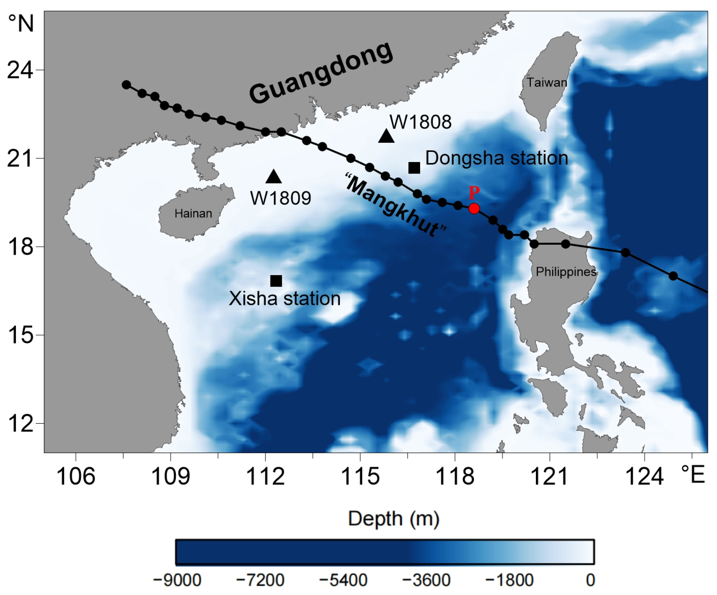
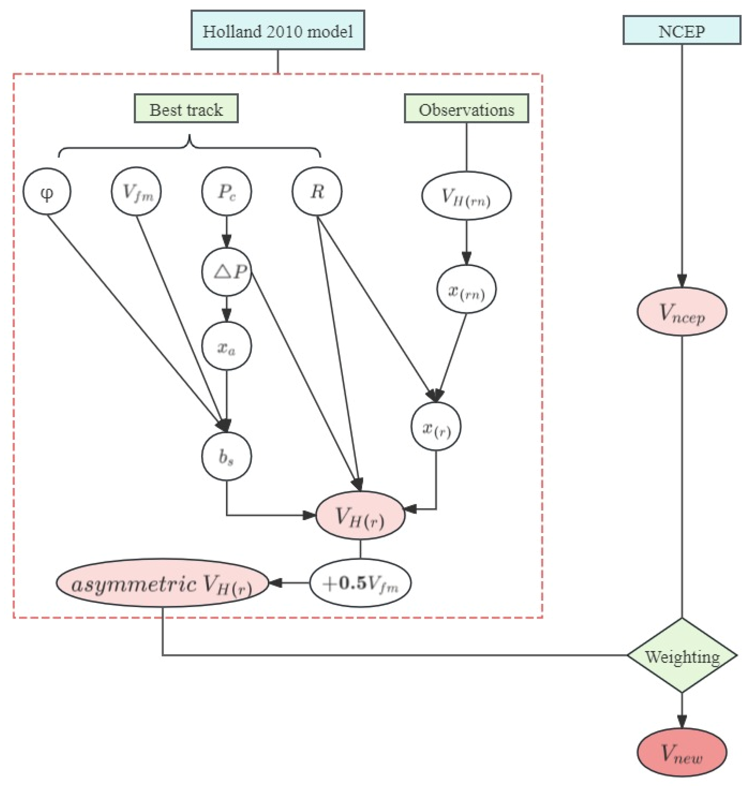
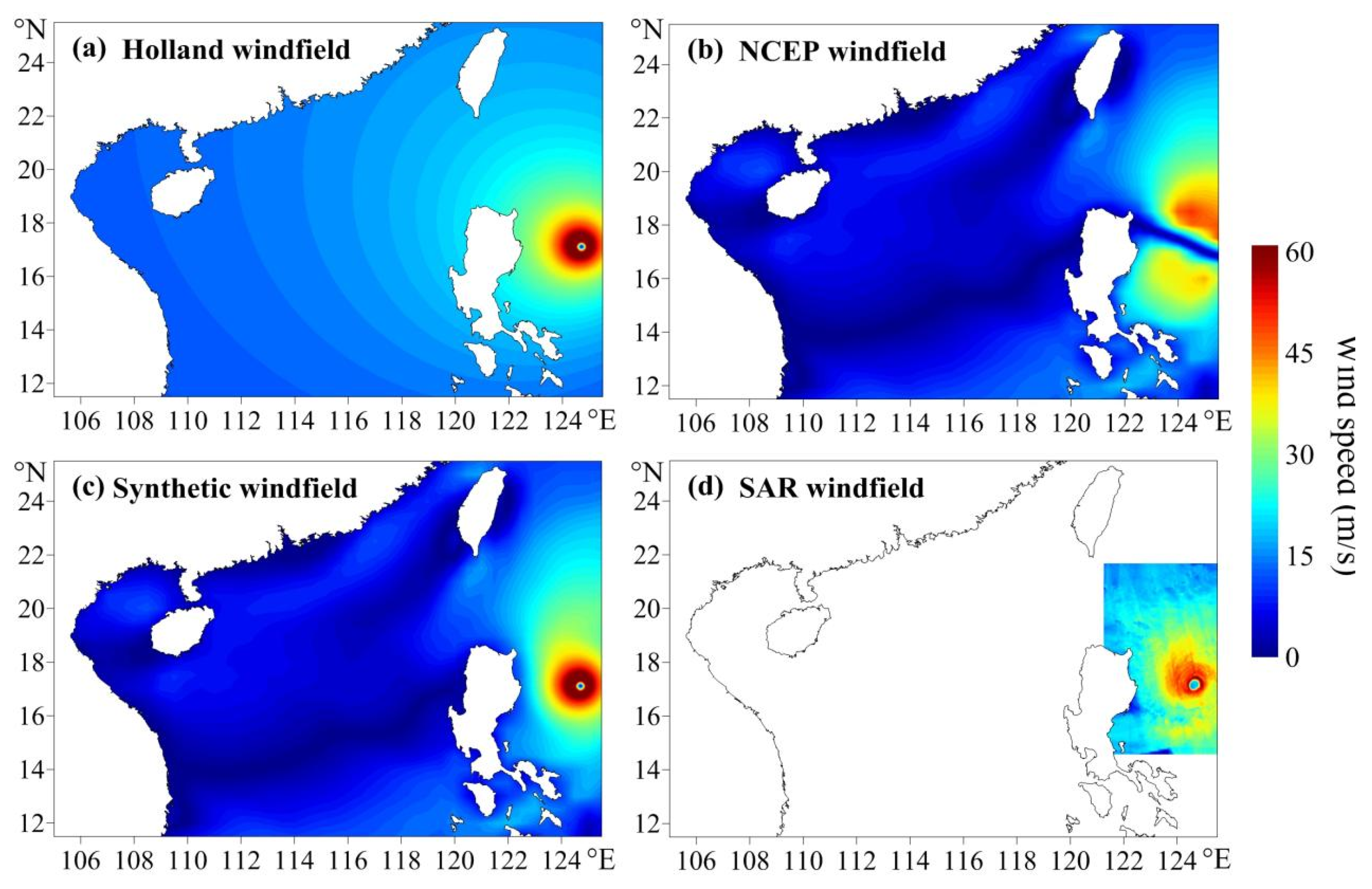
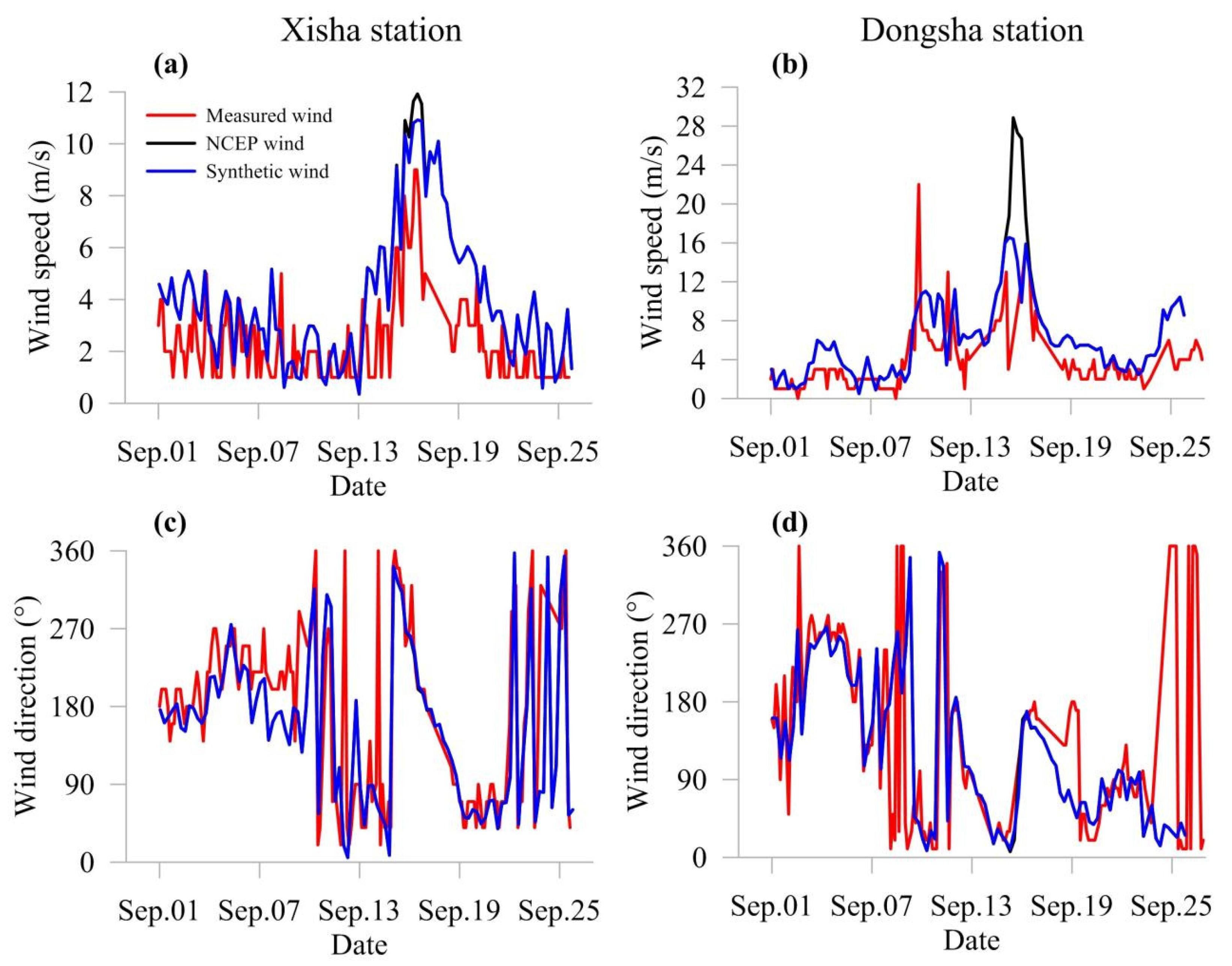
2.1. Construction of the Typhoon Wind Field
2.2. Model Setup
3. Results
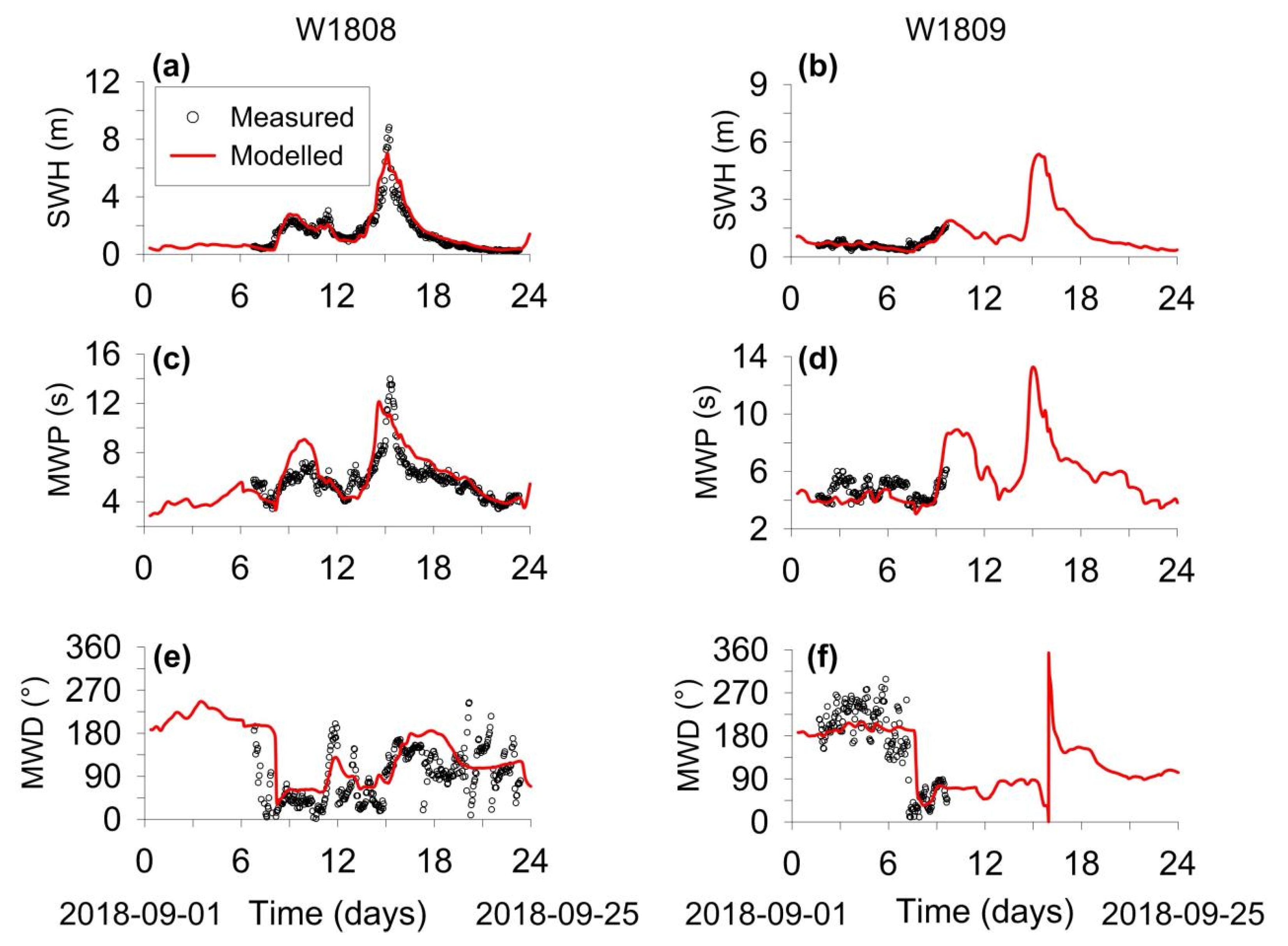
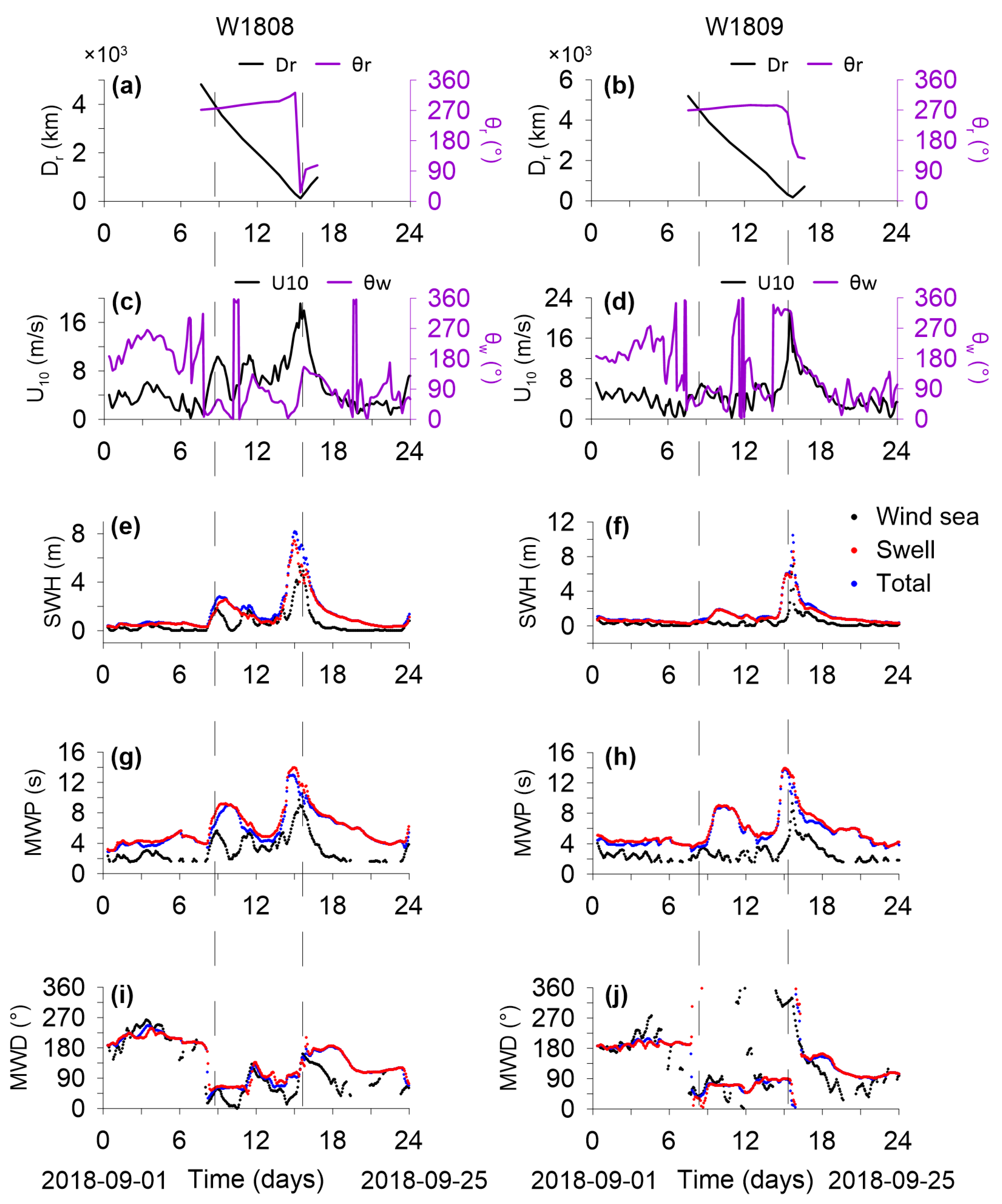
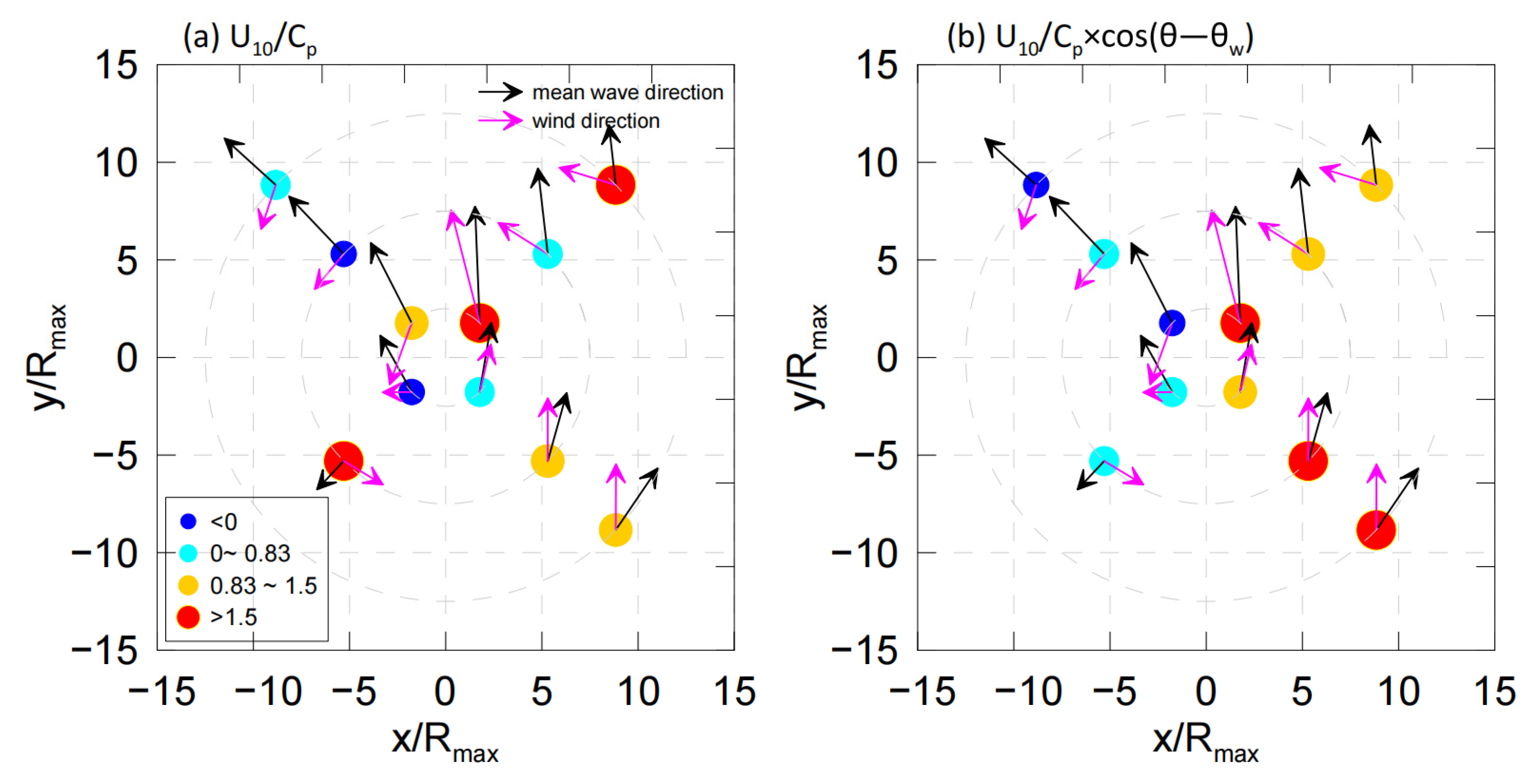
3.1. TW Parameters
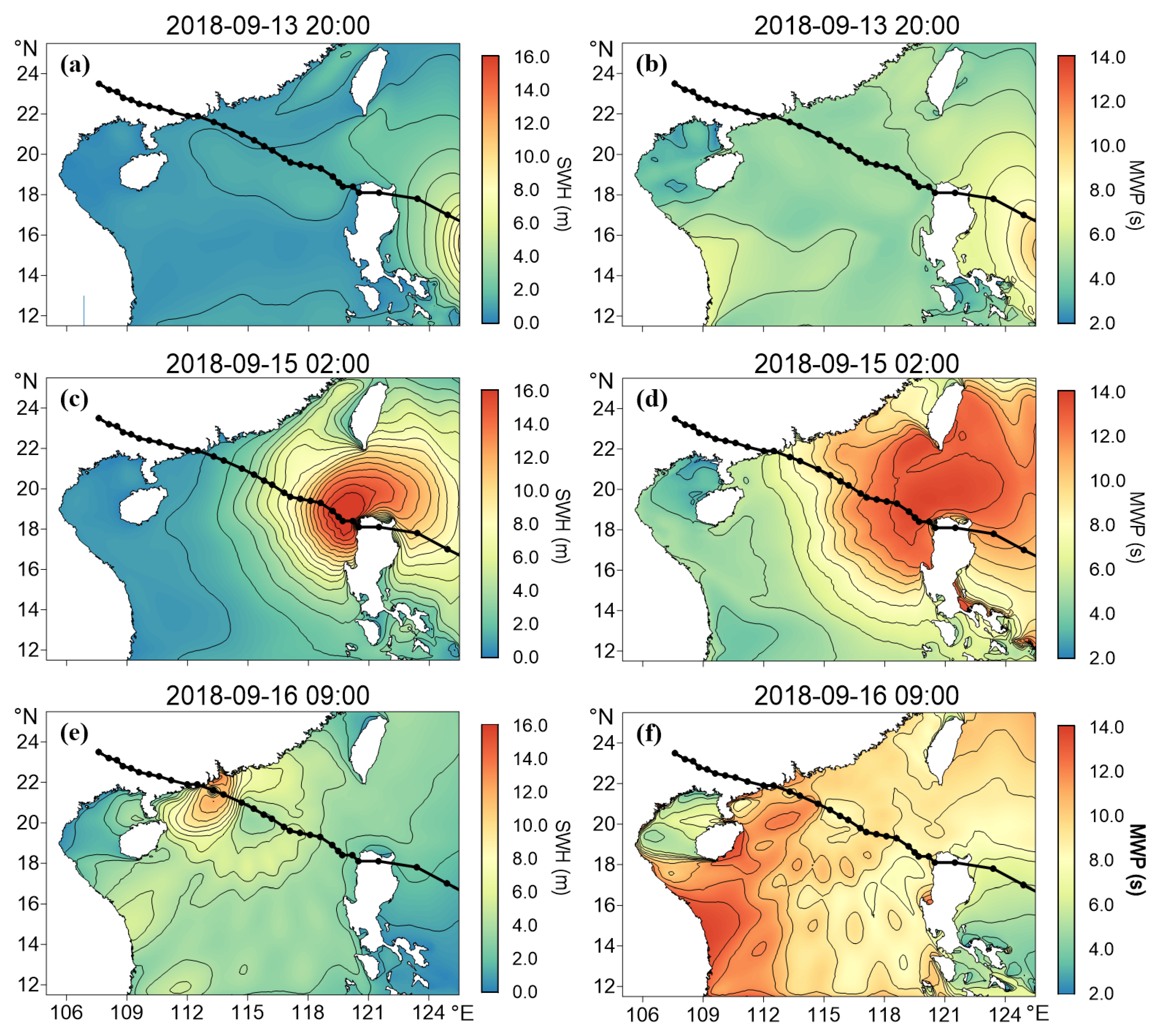
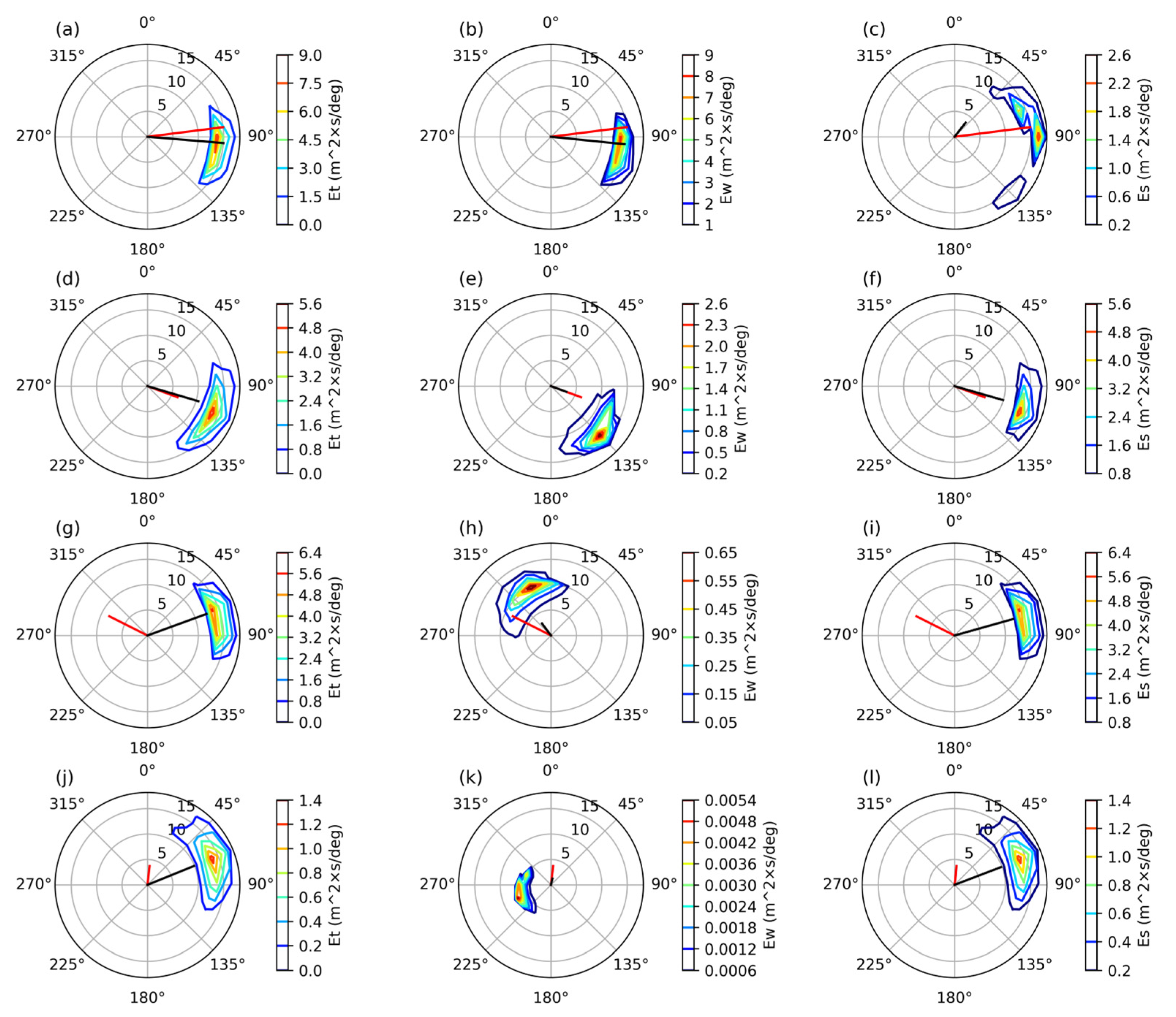
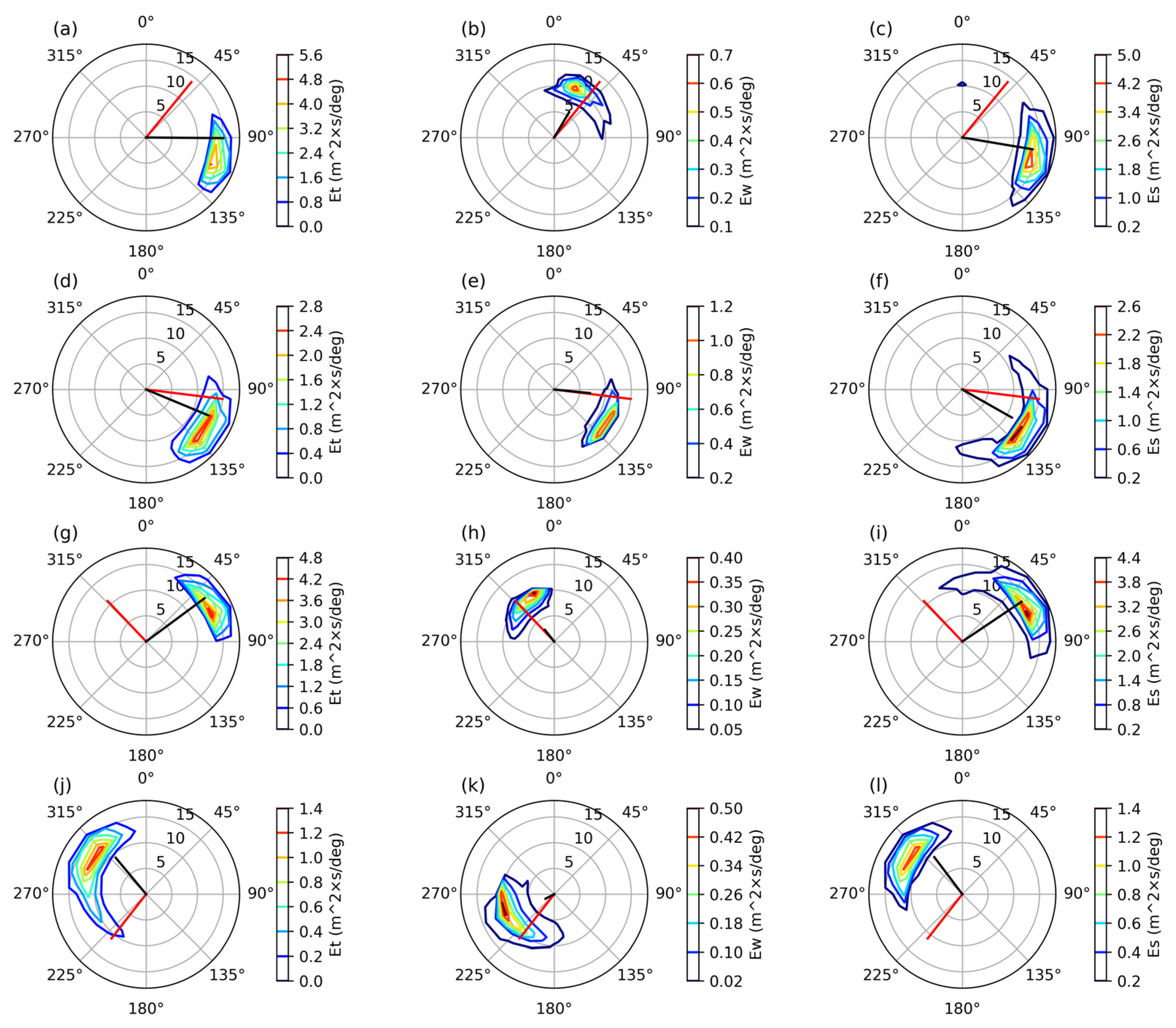
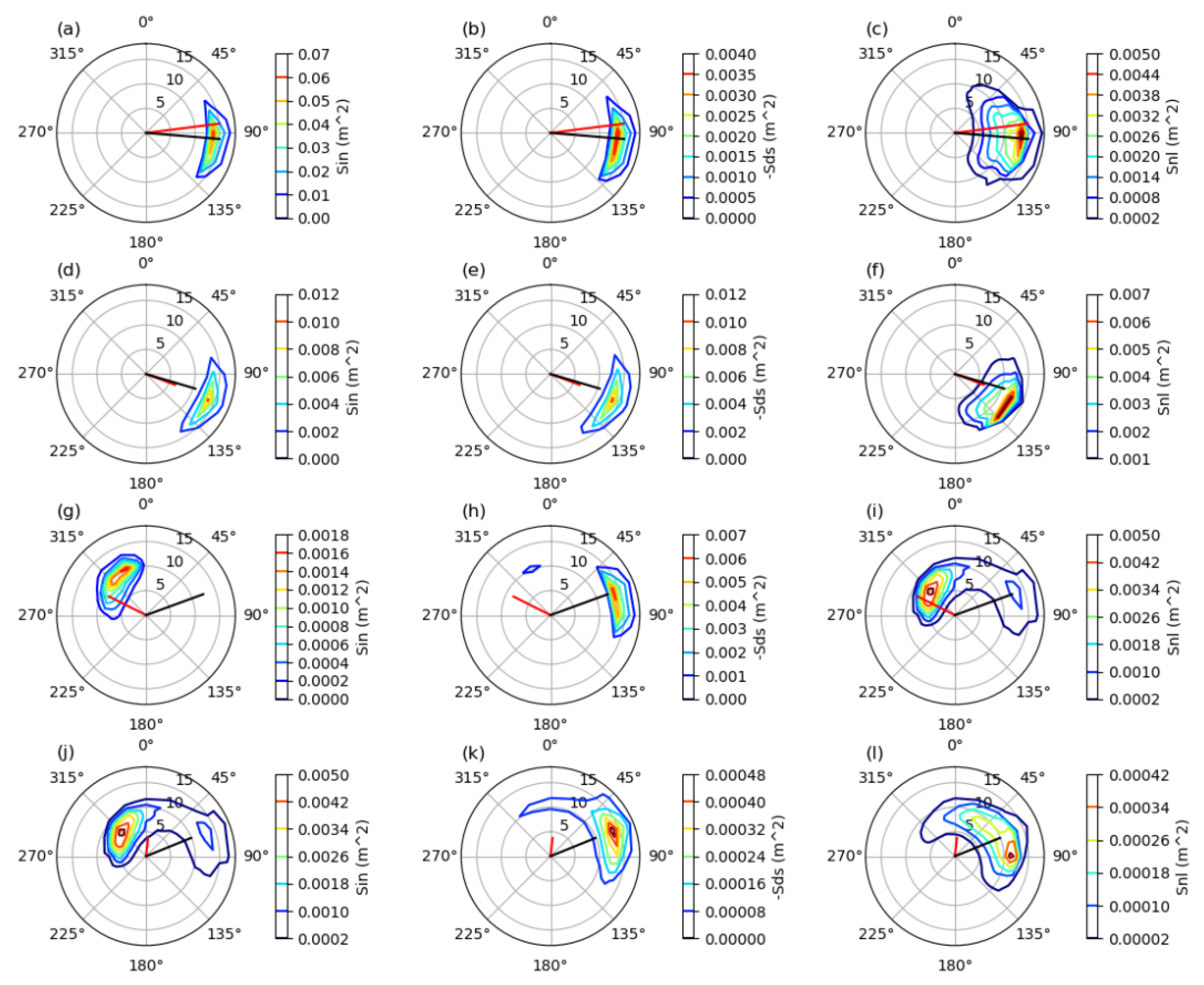
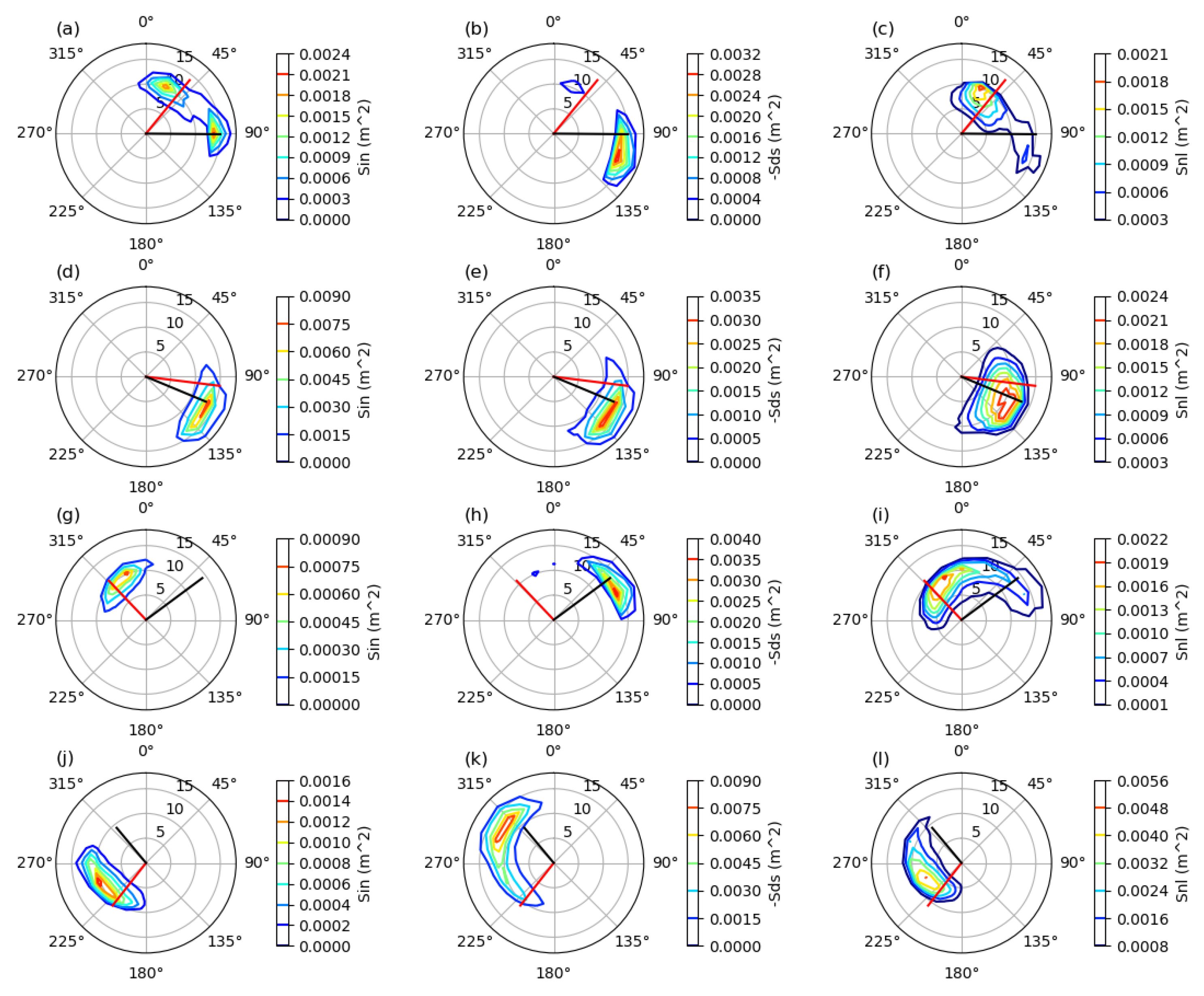
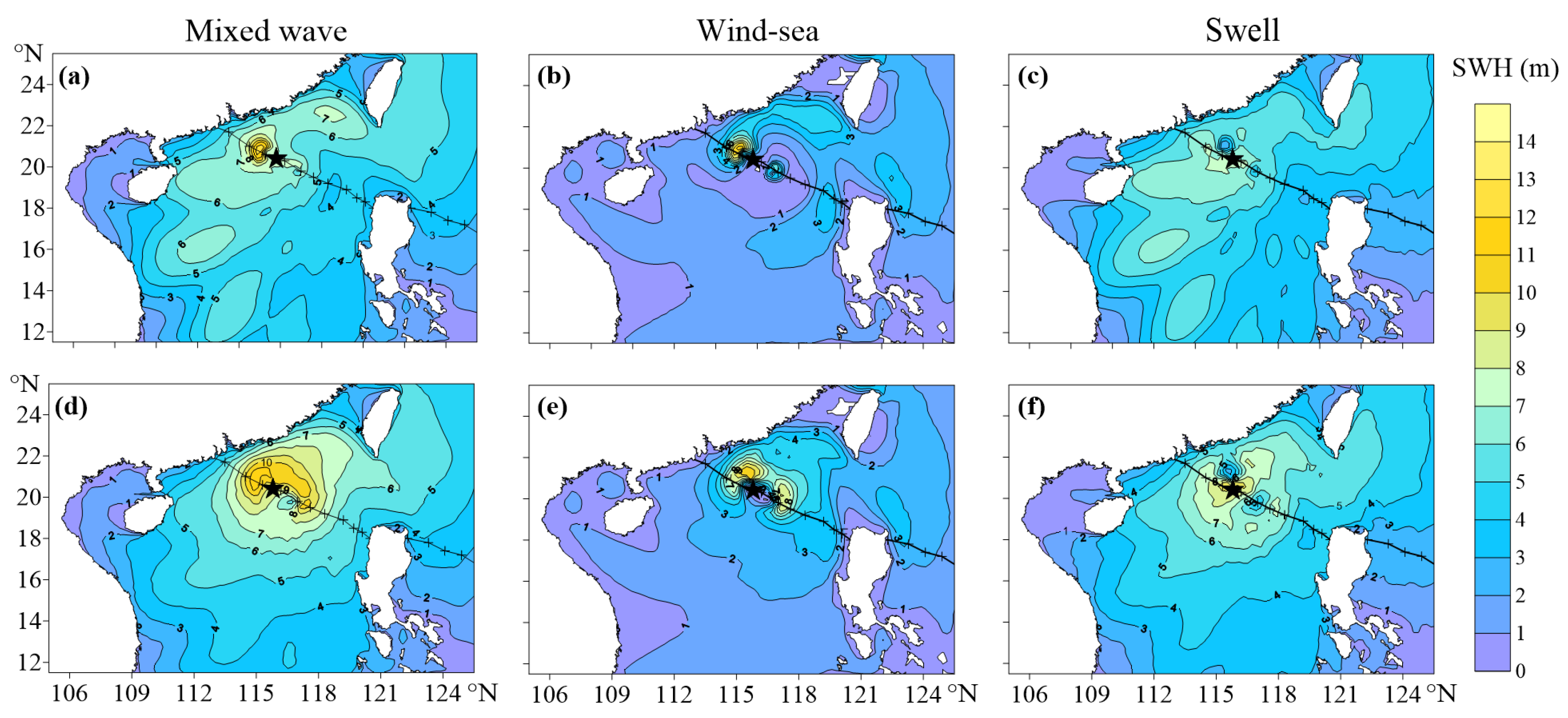
3.2. Spatial Distribution of the Wave Spectra
4. Discussion and Conclusions
Author Contributions
Funding
Institutional Review Board Statement
Informed Consent Statement
Data Availability Statement
Acknowledgments
Conflicts of Interest
References
- Forristall, G.Z.; Ward, E.G.; Cardone, V.J.; Borgmann, L.E. The directional spectra and kinematics of surface gravity waves in Tropical Storm Delia. J. Phys. Oceanogr. 1978, 8, 888–909. [Google Scholar] [CrossRef]
- Wright, C.W.; Walsh, E.J.; Vandemark, D.; Krabill, W.B.; Garcia, A.W.; Houston, S.H.; Powell, M.D.; Black, P.G.; Marks, F.D. Hurricane directional wave spectrum spatial variation in the open ocean. J. Phys. Oceanogr. 2001, 31, 2472–2488. [Google Scholar] [CrossRef]
- Walsh, E.J.; Wright, C.W.; Vandemark, D.; Krabill, W.B.; Garcia, A.W.; Houston, S.H.; Murillo, S.T.; Powell, M.D.; Black, P.G.; Marks, F.D. Hurricane directional wave spectrum spatial variation at landfall. J. Phys. Oceanogr. 2002, 32, 1667–1684. [Google Scholar] [CrossRef]
- Babovic, V.; Sannasiraj, S.A.; Chan, E.S. Error correction of a predictive ocean wave model using local model approximation. J. Mar. Syst. 2005, 53, 1–17. [Google Scholar] [CrossRef]
- Jain, P.; Deo, M.C. Real-time wave forecasts off the western Indian coast. Appl. Ocean Res. 2007, 29, 72–79. [Google Scholar] [CrossRef]
- Hwang, P.A.; Fan, Y. Effective fetch and duration of tropical cyclone wind fields estimated from simultaneous wind and wave measurements: Surface wave and air–sea exchange computation. J. Phys. Oceanogr. 2017, 47, 447–470. [Google Scholar] [CrossRef]
- Young, I.R. A review of parametric descriptions of tropical cyclone wind-wave generation. Atmosphere 2017, 8, 194. [Google Scholar] [CrossRef]
- Grossmann-Matheson, G.; Young, I.R.; Alves, J.; Meucci, A. Development and validation of a parametric tropical cyclone wave height prediction model. Ocean Eng. 2023, 283, 115353. [Google Scholar] [CrossRef]
- Ou, S.-H.; Liau, J.-M.; Hsu, T.-W.; Tzang, S.-Y. Simulating typhoon waves by SWAN wave model in coastal waters of Taiwan. Ocean Eng. 2002, 29, 947–971. [Google Scholar] [CrossRef]
- Rogers, W.E.; Kaihatu, J.M.; Hsu, L.; Jensen, R.E.; Dykes, J.; Holland, K.T. Forecasting and hindcasting waves with the SWAN model in the Southern California Bight. Coast. Eng. 2007, 54, 1–15. [Google Scholar] [CrossRef]
- Divinsky, B.V.; Kosyan, R.D. Parameters of wind seas and swell in the Black Sea based on numerical modeling. Oceanologia 2018, 60, 277–287. [Google Scholar] [CrossRef]
- Fonseca, R.B.; Gonçalves, M.; Guedes Soares, C. Comparing the performance of spectral wave models for coastal areas. J. Coast. Res. 2017, 33, 331–346. [Google Scholar] [CrossRef]
- Tang, J.; Shi, J.; Li, X.; Deng, B.; Jing, M. Numerical simulation of typhoon waves with typhoon wind model. Trans. Oceanol. Limnol. 2013, 2, 24–30. [Google Scholar]
- Allahdadi, M.N.; Chaichitehrani, N.; Allahyar, M.; McGee, L. Wave Spectral Patterns during a Historical Cyclone: A Numerical Model for Cyclone Gonu in the Northern Oman Sea. Open J. Fluid Dyn. 2017, 7, 131–151. [Google Scholar] [CrossRef]
- Pan, D.; Wan, J.; Zhou, C. Numerical simulation of wave based on Typhoon Mangkhut. J. Waterw. Harb. 2021, 42, P194–P199. (In Chinese) [Google Scholar]
- Xu, F.; Perrie, W.; Toulany, B.; Smith, P.C. Wind-generated waves in Hurricane Juan. Ocean Model. 2007, 16, 188–205. [Google Scholar] [CrossRef]
- Holland, J.G. An analytic model of the wind and pressure profiles in hurricanes. Mon. Weather Rev. 1980, 108, 1212–1218. [Google Scholar] [CrossRef]
- Willoughby, H.E.; Darling, R.W.R.; Rahn, M.E. Parametric representation of the primary hurricane vortex. Part II: A new family of sectionally continuous profiles. Mon. Weather Rev. 2006, 134, 1102–1120. [Google Scholar] [CrossRef]
- Holland, J.G. A revised hurricane pressure–wind model. Mon. Weather Rev. 2008, 136, 3432–3445. [Google Scholar] [CrossRef]
- Holland, J.G.; Belanger, I.J.; Fritz, A. A revised model for radial profiles of hurricane winds. Mon. Weather Rev. 2010, 12, 4393–4401. [Google Scholar] [CrossRef]
- Lin, N.; Chavas, D. On hurricane parametric wind and applications in storm surge modeling. J. Geophys. Res. Atmos. 2012, 117, D09120. [Google Scholar] [CrossRef]
- Xie, L.; Bao, S.; Pietrafesa, L.J.; Foley, K.; Fuentes, M. A real-time hurricane surface wind forecasting model: Formulation and verification. Mon. Weather Rev. 2006, 134, 1355–1370. [Google Scholar] [CrossRef]
- Liu, H.; Xie, L.; Pietrafesa, L.J.; Bao, S. Sensitivity of wind waves to hurricane wind characteristics. Ocean Model. 2007, 18, 37–52. [Google Scholar] [CrossRef]
- Zhang, J.; Uhlhorn, E.W. Hurricane sea surface inflow angle and an observation-based parametric model. Mon. Weather Rev. 2012, 140, 3587–3605. [Google Scholar] [CrossRef]
- Tamizi, A.; Young, I.R.; Ribal, A.; Alves, J.-H. Global scatterometer observations of the structure of tropical cyclone wind fields. Mon. Weather Rev. 2020, 148, 4673–4692. [Google Scholar] [CrossRef]
- Moon, I.J.; Ginis, I.; Hara, T.; Tolman, H.L.; Wright, C.W.; Walsh, E.J. Numerical simulation of sea surface directional wave spectra under Hurricane wind forcing. J. Phys. Oceanogr. 2003, 33, 1680–1706. [Google Scholar] [CrossRef]
- Young, I.R. Directional spectra of hurricane wind waves. J. Geophys. Res. 2006, 111, C8020. [Google Scholar] [CrossRef]
- Hu, K.; Chen, Q. Directional spectra of hurricane-generated waves in the Gulf of Mexico. Geophys. Res. Lett. 2011, 38, L19608. [Google Scholar] [CrossRef]
- Tamizi, A.; Young, I.R. The Spatial Distribution of Ocean Waves in Tropical Cyclones. J. Phys. Oceanogr. 2020, 50, 2123–2139. [Google Scholar] [CrossRef]
- Tamizi, A.; Alves, J.H.; Young, I.R. The Physics of Ocean Wave Evolution within Tropical Cyclones. J. Phys. Oceanogr. 2021, 7, 2373–2388. [Google Scholar] [CrossRef]
- King, D.B.; Shemdin, O.H. Radar observations of hurricane wave directions. In Proceedings of the 16th International Conference on Coastal Engineering, Hamburg, Germany, 27 August–3 September 1978. [Google Scholar]
- Young, I.R. Observations of the spectra of hurricane generated waves. Ocean Eng. 1998, 25, 261–276. [Google Scholar] [CrossRef]
- Li, M.; He, Y.; Liu, G. Atmospheric and oceanic responses to Super Typhoon Mangkhut in the South China Sea: A coupled CROCO-WRF simulation. J. Oceanol. Limnol. 2023, 41, 1369–1388. [Google Scholar] [CrossRef]
- Wu, Z.; Gao, K.; Chen, J.; Zhang, H.; Deng, B.; Jiang, C.; Liu, Y.; Lyu, Z.; Yan, R. Typhoon-induced ocean waves and stokes drift: A case study of Typhoon Mangkhut (2018). China Ocean Eng. 2024, 38, 711–724. [Google Scholar] [CrossRef]
- Zhang, Z.; Song, Z.; Zhang, D.; Hu, D.; Yu, Z.; Yue, S. Tide–surge interactions in Lingdingyang Bay, Pearl River Estuary, China: A case study from Typhoon Mangkhut, 2018. Estuaries Coasts 2024, 47, 330–351. [Google Scholar] [CrossRef]
- Komen, G.J.; Cavaleri, L.; Doneland, M.; Hasselmann, K.; Hasselmann, S.; Janssen PA, E.M. Dynamics and Modelling of Ocean Waves; Cambridge University Press: Cambridge, UK, 1994. [Google Scholar]
- Young, I.R. Wind Generated Ocean Waves; Elsevier Ocean Engineering Book Series; Bhattacharyya, R., McCormick, M.E., Eds.; Elsevier: Amsterdam, The Netherlands, 1999; Volume 2. [Google Scholar]
- Ris, R.C. Spectral Modelling of Wind Waves in Coastal Areas. Ph.D. Thesis, Delft University of Technology, Delft, The Netherlands, 1997. [Google Scholar]
- Janssen PA, E.M. Quasi-linear theory of wind wave generation applied to wave forecasting. J. Phys. Oceanogr. 1991, 21, 1631–1642. [Google Scholar] [CrossRef]
- Hasselmann, K. On the spectral dissipation of ocean waves due to white capping. Bound.-Layer Meteorol. 1974, 6, 107–127. [Google Scholar] [CrossRef]
- Janssen PA, E.M. Wave induced stress and the drag of airflow over sea waves. J. Phys. Oceanogr. 1989, 19, 745–754. [Google Scholar] [CrossRef]
- Hasselmann, S.; Hasselmann, K. Computation and parameterizations of non-linear energy transfer in a gravity-wave spectrum, part 1: A new method for efficient computations of the exact non-linear transfer integral. J. Phys. Oceanogr. 1985, 15, 1369–1377. [Google Scholar] [CrossRef]
- Komen, G.J.; Hasselmann, K.; Hasselmann, K. On the existence of a fully developed wind-sea spectrum. J. Phys. Oceanogr. 1984, 14, 1271–1285. [Google Scholar] [CrossRef]
- Schloemer, R.W. Analysis and Synthesis of Hurricane Wind Patterns over Lake Okechobee, Florida; Hydromet. Rep. 31; US Department of Commerce: Washington, DC, USA, 1954.
- Kalourazi, M.Y.; Siadatmousavi, S.M.; Yeganeh-Bakhtiary, A.; Jose, F. WAVEWATCH-III source terms evaluation for optimizing hurricane wave modeling: A case study of Hurricane Ivan. Oceanologia 2021, 63, 194–213. [Google Scholar] [CrossRef]
- Carr, L.E., III; Elsberry, R.L. Models of tropical cyclone wind distribution and Beta-effect propagation for application to tropical cyclone track forecasting. Mon. Weather Rev. 1997, 125, 3190–3209. [Google Scholar] [CrossRef]
- Zhang, Z.; Qi, Y.; Shi, P.; Li, C. Application of an optimal interpolation wave assimilation method in South China Sea. J. Trop. Oceanogr. 2003, 4, 34–41. (In Chinese) [Google Scholar]
- Xu, Y.; He, H.; Song, J.; Hou, Y.; Li, F. Observations and modeling of typhoon waves in the South China Sea. J. Phys. Oceanogr. 2017, 47, 1307–1324. [Google Scholar] [CrossRef]
- Donelan, M.A.; Hamilton, J.; Hui, W.H. Directional spectra of wind-generated waves. Philos. Trans. R. Soc. Lond. Ser. A 1985, 315, 509–562. [Google Scholar]
- Hasselmann, K.; Barnett, T.P.; Bouws, E.; Carlson, H.; Cartwright, D.E.; Enke, K.; Ewing, J.A.; Gienapp, A.; Hasselmann, D.E.; Kruseman, P.; et al. Measurements of wind wave growth and swell decay during the Joint North Sea Wave Project (JONSWAP). Dtsch. Hydrogr. Z. 1973, 8A, 95. [Google Scholar]
- Young, I.R. Parametric hurricane wave prediction model. J. Waterw. Port Coast. Ocean Eng. 1988, 114, 637–652. [Google Scholar] [CrossRef]
- Young, I.R.; Burchell, G.P. Hurricane generated waves as observed by satellite. Ocean Eng. 1986, 23, 761–776. [Google Scholar] [CrossRef]
- Young, I.R.; Vinoth, J. An ‘extended fetch’ model for the spatial distribution of tropical cyclone wind-waves as observed by altimeter. Ocean Eng. 2013, 70, 14–24. [Google Scholar] [CrossRef]

| N | Quadrant | r | ||||||
|---|---|---|---|---|---|---|---|---|
| 1 | right–forward | 2.5 Rmax | 94.71 | 82.76 | 31.82 | 12.55 | 0.98 | 18.58 |
| 2 | right–rear | 2.5 Rmax | 106.51 | 110.29 | 13.37 | 8.75 | 1.00 | 4.59 |
| 3 | left–forward | 2.5 Rmax | 69.94 | 296.74 | 17.83 | 10.35 | −0.68 | −22.56 |
| 4 | left–rear | 2.5 Rmax | 67.90 | 6.39 | 7.88 | 8.26 | 0.48 | −4.50 |
| 5 | right–forward | 7.5 Rmax | 90.46 | 39.22 | 15.96 | 10.07 | 0.63 | −0.08 |
| 6 | right–rear | 7.5 Rmax | 112.59 | 97.05 | 17.17 | 8.80 | 0.96 | 7.75 |
| 7 | left–forward | 7.5 Rmax | 53.45 | 316.52 | 12.45 | 9.50 | −0.12 | −11.00 |
| 8 | left–rear | 7.5 Rmax | 320.13 | 218.09 | 12.51 | 6.18 | −0.21 | −8.79 |
Disclaimer/Publisher’s Note: The statements, opinions and data contained in all publications are solely those of the individual author(s) and contributor(s) and not of MDPI and/or the editor(s). MDPI and/or the editor(s) disclaim responsibility for any injury to people or property resulting from any ideas, methods, instructions or products referred to in the content. |
© 2024 by the authors. Licensee MDPI, Basel, Switzerland. This article is an open access article distributed under the terms and conditions of the Creative Commons Attribution (CC BY) license (https://creativecommons.org/licenses/by/4.0/).
Share and Cite
Yan, Y.; Hu, M.; Ni, Y.; Qiu, C. Simulated Directional Wave Spectra of the Wind Sea and Swell under Typhoon Mangkhut. Atmosphere 2024, 15, 1174. https://doi.org/10.3390/atmos15101174
Yan Y, Hu M, Ni Y, Qiu C. Simulated Directional Wave Spectra of the Wind Sea and Swell under Typhoon Mangkhut. Atmosphere. 2024; 15(10):1174. https://doi.org/10.3390/atmos15101174
Chicago/Turabian StyleYan, Yu, Mengxi Hu, Yugen Ni, and Chunhua Qiu. 2024. "Simulated Directional Wave Spectra of the Wind Sea and Swell under Typhoon Mangkhut" Atmosphere 15, no. 10: 1174. https://doi.org/10.3390/atmos15101174