Article

Source Attribution Analysis of an Ozone Concentration Increase Event in the Main Urban Area of Xi’an Using the WRF-CMAQ Model

1
College of New Energy and Environment, Jilin University, Changchun 130012, China
2
Key Laboratory of Groundwater Resources and Environment, Ministry of Education, Jilin University, Changchun 130012, China
3
Jilin Province Key Laboratory of Water Resources and Environment, Jilin University, Changchun 130012, China
*
Author to whom correspondence should be addressed.
Atmosphere 2024, 15(10), 1208; https://doi.org/10.3390/atmos15101208
Submission received: 3 September 2024 / Revised: 3 October 2024 / Accepted: 8 October 2024 / Published: 10 October 2024
(This article belongs to the Section Air Quality)

Abstract

:
The significant increase in ambient ozone (O3) levels across China highlights the urgent need to investigate the sources and mechanisms driving regional O3 events, particularly in densely populated urban areas. This study focuses on Xi’an, located in northwestern China on the Guanzhong Plain near the Qinling Mountains, where the unique topography contributes to pollutant accumulation. Urbanization and industrial activities have significantly increased pollutant emissions. Utilizing the Weather Research and Forecasting–Community Multiscale Air Quality Model (WRF-CMAQ), we analyzed the contributions of specific regional and industrial sources to rising O3 levels, particularly during an atypical winter event characterized by unusually high concentrations. Our findings indicated that boundary conditions were the primary contributor to elevated O3 levels during this event. Notably, Xianyang and Baoji accounted for 30% and 22% of the increased O3 levels in Xi’an, respectively. Additionally, residential sources and transportation accounted for 31% and 28% of the O3 increase. Within the Xi’an metropolitan area, Baqiao District (18–27%) and Weiyang District (23–30%) emerged as leading contributors. The primary industries contributing to this rise included residential sources (28–37%) and transportation (35–43%). These insights underscore the need for targeted regulatory measures to mitigate O3 pollution in urban settings.

1. Introduction

O3 is produced through a complex chemical reaction involving volatile organic compounds (VOCs) and nitrogen oxides (NOx) when exposed to light [1]. The strong oxidizing properties of O3 can cause varying degrees of harm to organisms, plants, crops, and humans at different concentrations [2,3,4,5,6,7].
Favorable meteorological conditions can enhance O3 transport, increasing exposure and associated health risks [8]. Identifying sources of O3 is crucial for developing effective control measures. A significant challenge is quantifying contributions and processes across different scales. The WRF-CMAQ model is an effective tool for studying O3 contributions and transport. Chen et al. [9] examined O3 seasonality in southern China’s coastal region, noting that O3 sources are primarily classified into local contributions and regional transport, with pollution peaking in spring and summer. Wang et al. [10] utilized the WRF-CMAQ model to simulate O3 pollution events in the Yangtze River Delta in 2018. The results indicated that the source tracking of O3 and volatile organic compounds (VOCs) using the integrated source analysis method (ISAM) in the CMAQ model accurately reflected actual pollution sources and their contributions. The basin’s unique topography facilitates slow air movement and pollutant accumulation [11,12,13], making it a subject of extensive research. Yang et al. [14] simulated a pollution event in the Sichuan Urban Agglomeration in 2018 using the WRF-CMAQ modeling system. They employed the ISAM to investigate a severe O3 event in the SCB region during spring 2020, attributed to localized emissions and regional transport under unfavorable meteorological conditions. Most studies of O3 pollution focus on spring and summer [15,16], periods characterized by high temperatures, solar radiation, photochemical pollution, and O3 concentrations. However, few studies have examined the phenomenon and causes of elevated O3 concentrations in winter [17].
Xi’an, situated in the Guanzhong Plain, is a key city and energy center in Central and Western China, making it a focal point for air-pollution control [18,19]. Yan et al. [13] examined typical weather circulation types (CTs) related to summer O3 pollution and assessed their impacts on O3 sources in the Guanzhong Basin using observational data and model simulations. The results indicated that O3 pollution in Xi’an is significantly influenced by local contributions and external transport, while intra-regional and extra-urban emissions also play a crucial role. Feng et al. [20] and Han et al. [21] analyzed the concentrations of six pollutants and air quality in Xi’an in 2020 using observational data and natural experiments. Their results revealed decreases in the AQI and concentrations of PM2.5, PM10, SO2, and CO, with NO2 decreasing by 52% while O3 concentrations rose by 160% due to reduced motor vehicle emissions. Other studies indicate that the increased traffic volume in Xi’an has raised VOCs and NOx concentrations, worsening O3 pollution [22,23,24]. Most studies have primarily examined the correlation between O3 levels and meteorological factors, often overlooking geographic and socio-economic influences and their synergistic and counteracting effects. Additionally, Xi’an is recognized as a hazy city, with numerous studies focusing on particulate matter, VOCs, NOx, and air-quality changes [18,25,26,27,28]. The WRF-CMAQ model has been employed to track O3 concentrations in Xi’an. Utilizing the WRF-CMAQ model to trace regional and sectoral emissions of O3 in Xi’an represents a novel approach for attributing changes in O3 concentrations. Our study employed three nested layers, conducting simultaneous source analyses of the second layer (Guanzhong city cluster) and the third layer (Xi’an urban area) to compare with February 2019. This allowed us to identify which cities and industries in the second layer, serving as boundary conditions for the third layer, contributed most to O3 concentrations in Xi’an during mid-February 2020. We also identified the regions and industries in Xi’an that significantly contributed to O3 concentrations, investigating the primary reasons for the observed increase in February 2020. Our findings offer valuable insights for future O3 control policies. Section 2 details the data and methodology, Section 3 presents the model configuration and evaluation, and Section 4 summarizes the conclusions and prospects.

2. Data and Methods

2.1. Data Sources

This study collected hourly O3 concentration data for February 2019 and 2020, expressed in μg/m3. The data were obtained from the National Urban Air Quality Real-Time Dissemination Platform, Ministry of Ecology and Environment (accessed 5 July 2022). Meteorological data for 2019 and 2020 were acquired from the China Meteorological Data Service Center (accessed 5 July 2022). The Xi’an urban area contains 15 automatic atmospheric monitoring stations, including the High Voltage Switch Plant (HVSP), Xingqing District (XQ), Textile City (TC), Xiaozhai (XZ), Municipal People’s Stadium (PS), Gaoxin West (GXW), Jingkai District (EDZ), Chang’an District (CA), Yanliang District (YL), Lintong District (LT), Caotan (CT), Qiujiang Cultural Industry Group (QJC), Cultural and Sports Bureau (CBS), and Radio Monitoring Center (RMC). Caotan (CT) functions as the control site, while CBS and RMC were newly established in 2022 and 2023 and thus lacked the data required for this study. The Jing He station supplied the meteorological data for this study. Table S1 presents the details regarding each monitoring station.

2.2. Model Application

2.2.1. WRF-CMAQ

The WRF-CMAQ is an integrated environmental model that combines weather forecasting with air-quality simulations. The model consists of the following two main components: the WRF and CMAQ models. The WRF model is a highly customizable weather forecasting tool, suitable for both small- and large-scale forecasts, and is compatible with other models. The CMAQ model simulates air quality by assessing pollutant sources, transport, and their impacts on environmental health and ecosystems. By combining WRF and CMAQ, the WRF-CMAQ model delivers accurate and comprehensive weather and air-quality forecasts, relevant to fields such as climate change, air-quality management, and ecosystem studies.
In this study, the CMAQ model (v4.6.0), driven by the WRF model (v4.6.0), was utilized. The nested domains were established using the Inventory Spatial Allocation Tool (ISAT v2.0) prior to the simulation [29]. The WRF model employed the Lambert projected coordinate system, with a central latitude of 34.4° N and longitude of 108.7° E. The physical process parameter schemes applied in the WRF simulations are detailed in Table 1. A three-layer nested simulation was conducted, as shown in Figure 1, illustrating the nested structure of the study area. The first layer encompassed Central China, with a grid resolution of 27 km × 27 km; the second layer covered Shaanxi Province, with a resolution of 9 km × 9 km; and the third layer focused on the main urban area of Xi’an city, with a resolution of 3 km × 3 km. The initial and boundary meteorological conditions of WRF were derived from National Centers for Environmental Prediction (NCEP) final analysis (FNL) data, with a temporal resolution of 6 h and a spatial resolution of 1.0° × 1.0°.
The gridded emission inventory for the CMAQ model was based on the 2019 China Multiscale Emission Inventory (MEIC v1.4; 25 km × 25 km) developed by the MEIC team at Tsinghua University [37] (http://meicmodel.org.cn (accessed on 19 January 2024)). This inventory encompasses mainland China and includes emission data from the following five key sectors: power, industry, civil, transportation, and agriculture. The recorded pollutants include SO2, NOx, CO, NMVOC, NH3, PM2.5, BC, OC, and CO2. Emissions are allocated based on factors such as population, GDP, and road-land-use raster data, which are sourced from the Center for Resource and Environmental Science and Data at the Chinese Academy of Sciences (https://www.resdc.cn/ (accessed on 4 January 2024)). The MEIC emission inventory was processed using the Modular Emission Inventory Allocation Tools for the Community Multiscale Air Quality Model (MEIAT-CMAQ).

2.2.2. CMAQ-ISAM

ISAM is a marker-based source-assignment method commonly used with CMAQ to track pollutant sources, especially primary and secondary pollutants. Labeled species are incorporated into the chemical transport module for calculations related to atmospheric chemistry and physical processes. Kwok et al. [38] applied ISAM to model the contributions of nine source categories to O3 concentrations in California, comparing the results with those from the brute-force method. They found a correlation greater than 0.9 between the two methods, except for biological sources.
ISAM employs the following two labeling methods: area labeling and emission source labeling. When labeled pollutants enter the chemical transport module, chemical mechanisms generate different O3 concentration ratios using various labeled pollutants as reactants. Therefore, labeled emission sources can be considered to be O3 sources, despite O3 not being a primary pollutant [39]. In this study, we tracked regional and industrial emissions across six urban areas in Xi’an and five neighboring cities. The sources were categorized into the following five sectors: agriculture, industry, electricity, residential, and transportation. The MEIC list provides only agricultural ammonia emissions, and as NH3 is already included in the main CMAQ module, it does not contribute to gas-phase chemical simulations. Consequently, agricultural emissions do not contribute to O3 concentrations. Based on similar studies as well as Cao et al. [40], agricultural sources in the MEIC list were excluded from the ISAM O3 source analysis conducted in this study.

3. Results and Discussion

3.1. Characterization of O3 Concentration Based on Observed Data

Xi’an is situated in the Guanzhong Plain, which is characterized by a warm temperate semi-humid continental monsoon climate. In winter, lower temperatures and stable atmospheric conditions prevail, with atmospheric circulation dominated by westerly winds and stagnant meteorological conditions. During winter, westerly winds typically blow toward Xi’an from the northwest or southwest. The frequency of stagnant winds has increased, particularly during the heating season, when pollutant emissions are higher and less likely to disperse. Reduced solar radiation enables pollutants such as NO2 and CO to convert into secondary particulate matter, resulting in relatively low O3 concentrations. In this study, we processed O3 observation data from six ground stations in Xi’an by removing outliers and averaging the results. We observed a significant increase in the O3 concentration in February 2020 compared with the same month’s data from 2019 to 2022 (Figure 2). The monthly average O3 concentrations for February were 35 μg/m3 in 2019, 32 μg/m3 in 2021, and 42 μg/m3 in 2022. However, in February 2020, the average concentration reached 64 μg/m3, nearly double the levels observed in other years. The daily mean O3 concentration in February exhibited a “W” pattern in 2019, 2021, and 2022; however, this pattern was absent in 2020. Although the COVID-19 lockdown occurred between 2020 and 2022, the data did not reflect a natural year effect of the pandemic. O3 concentrations in 2019 were similar to those in 2021 and 2022; however, concentrations increased in 2020, suggesting that the COVID-19 lockdown was not responsible for the elevated O3 levels in that year. Consequently, analyzing the sources of elevated O3 concentrations in Xi’an in February 2020 could help to explain the phenomenon of higher concentrations during a period of reduced pollution.

3.2. Model Evaluation Performance

To ensure the accuracy of simulation results, WRF simulations are generally validated using the standardized mean error (NME), standardized mean bias (NMB), correlation coefficient (R), and index of agreement (IOA). CMAQ simulations are validated using the mean fractional bias (MFB), mean fractional error (MFE), correlation coefficient (R), and index of agreement (IOA). In previous studies, WRF simulations were deemed to meet performance criteria if the NMB was ≤±30%, NME was ≤50%, and R was ≥0.40 [41]. For CMAQ simulations, Boylan et al. [42] proposed that a model is excellent when the MFB is ≤±30% and MFE is ≤±50%. A model is deemed acceptable if the MFB is ≤±60% and MFE is ≤±75%. An IOA ≥ 0.50 indicates good consistency between the model’s simulation results and the actual data. N represents the number of samples, P i denotes the simulation result at the i-th moment, O i represents the monitoring result at the i-th moment, P ¯ is the mean value of the simulation results, and O ¯ is the mean value of the monitoring results.
The formulas for these five indicators are presented below:
R = i = 1 N P i P ¯ O i O ¯ i = 1 N P i P ¯ 2   i = 1 N P i P ¯ 2
N M B = i = 1 N P i O i i = 1 N O i
N M E = i = 1 N P i O i i = 1 N O i
M F B = 1 N i = 1 N P i O i ( O i + P i ) / 2
M F E = 1 N i = 1 N P i O i ( O i + P i ) / 2
I O A = 1 i = 1 N P i O i 2 i = 1 N P i O ¯ + O i + O ¯ 2  

3.2.1. Evaluation of WRF Performance

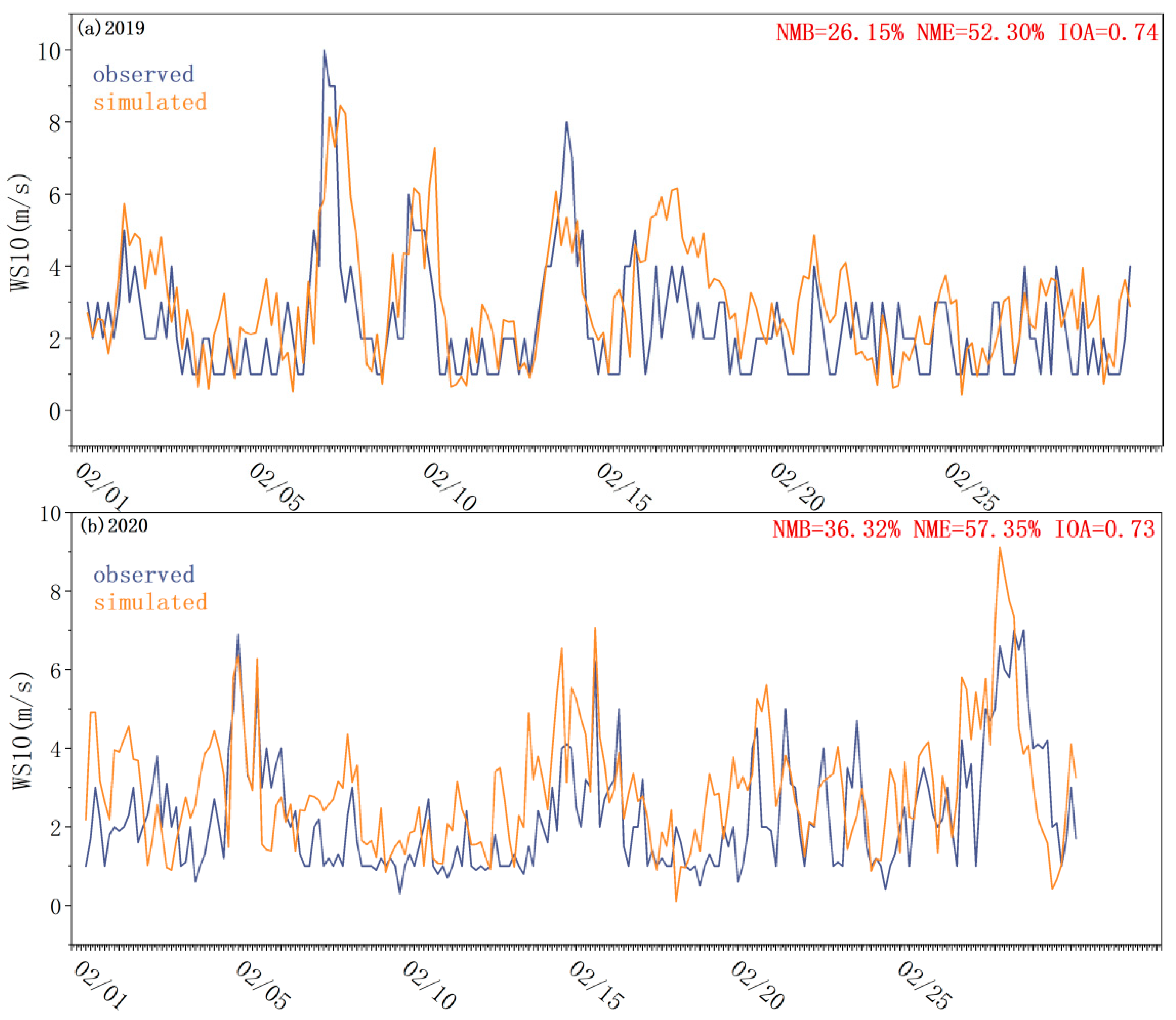
Meteorological factors significantly influence pollutant concentrations, and the accuracy of meteorological field simulations directly impacts the reliability of CMAQ results. Therefore, we first assessed the WRF-simulated meteorological fields. In this study, we conducted basic simulations for Xi’an in February 2019 and 2020, verifying and analyzing the simulation results for both months. The selected meteorological indicators included a 2 m temperature (T2) and a 10 m wind speed (WS10). A comparison of the WRF model simulations and the monitoring results is shown in Table 2 as well as Figure 3 and Figure 4.
Time-series comparisons of the simulated and observed meteorological parameters for February 2019 and 2020 in Xi’an are shown in Figure 3 and Figure 4. Figure 3 illustrates that the WRF model effectively captured T2 variations at the meteorological stations. The NMB and NME met the model performance criteria, with an R-value above 0.4 and an IOA exceeding 0.9. This indicated a strong agreement between the simulated and observed temperatures, demonstrating the model’s capability to replicate daily variations and trends in T2.
Figure 4 illustrates that the WRF model effectively captured WS10 variations at the meteorological stations. The WRF simulation effectively captured the peaks and troughs of WS10, with the NMB and NME meeting the performance criteria. The R-value exceeded 0.4 and the IOA was above 0.6, indicating strong usability of the WS10 simulation results. The overestimation of WS10 is a common characteristic of the model, especially in complex terrains [43,44]. An R-value of 0.7 for WS10 is typically regarded to be indicative of high simulation accuracy.

3.2.2. CMAQ Performance Evaluation

To ensure model performance stability, O3 concentration data from the CMAQ simulation were compared with observational data from environmental monitoring stations during the same period as the WRF model simulation. Hourly O3 data from national air-quality monitoring stations in Xi’an were statistically compared with the CMAQ model results, as illustrated in Figure 5. Table 3 displays the statistical comparison of the simulated and observed O3 concentrations. The comparison of the simulated and observed O3 values indicated that the simulation fell within an acceptable range (MFB ≤ ±30%, MFE ≤ ±75%, and IOA = 0.79 for February 2019; MFB ≤ ±30%, MFE ≤ ±50%, and IOA = 0.62 for February 2020). This demonstrated good consistency between the model and actual observations, accurately reflecting the changes in O3 concentrations. Figure 5 illustrates that the CMAQ model effectively captured peak pollutant changes, demonstrating strong consistency between the observed and simulated trends. However, the generally lower simulated values contributed to the low R-value. This discrepancy may have arisen from differences between the reported and actual emissions as well as mismatches in temporal and spatial allocation factors within the inventory [27]. Although the CMAQ model slightly underestimated the monitoring data, it successfully passed the validation tests, demonstrating good agreement with the pollutant concentration trends. Therefore, it was suitable for a further analysis of changes in O3 concentrations within the study area.

3.3. Source Analysis of O3

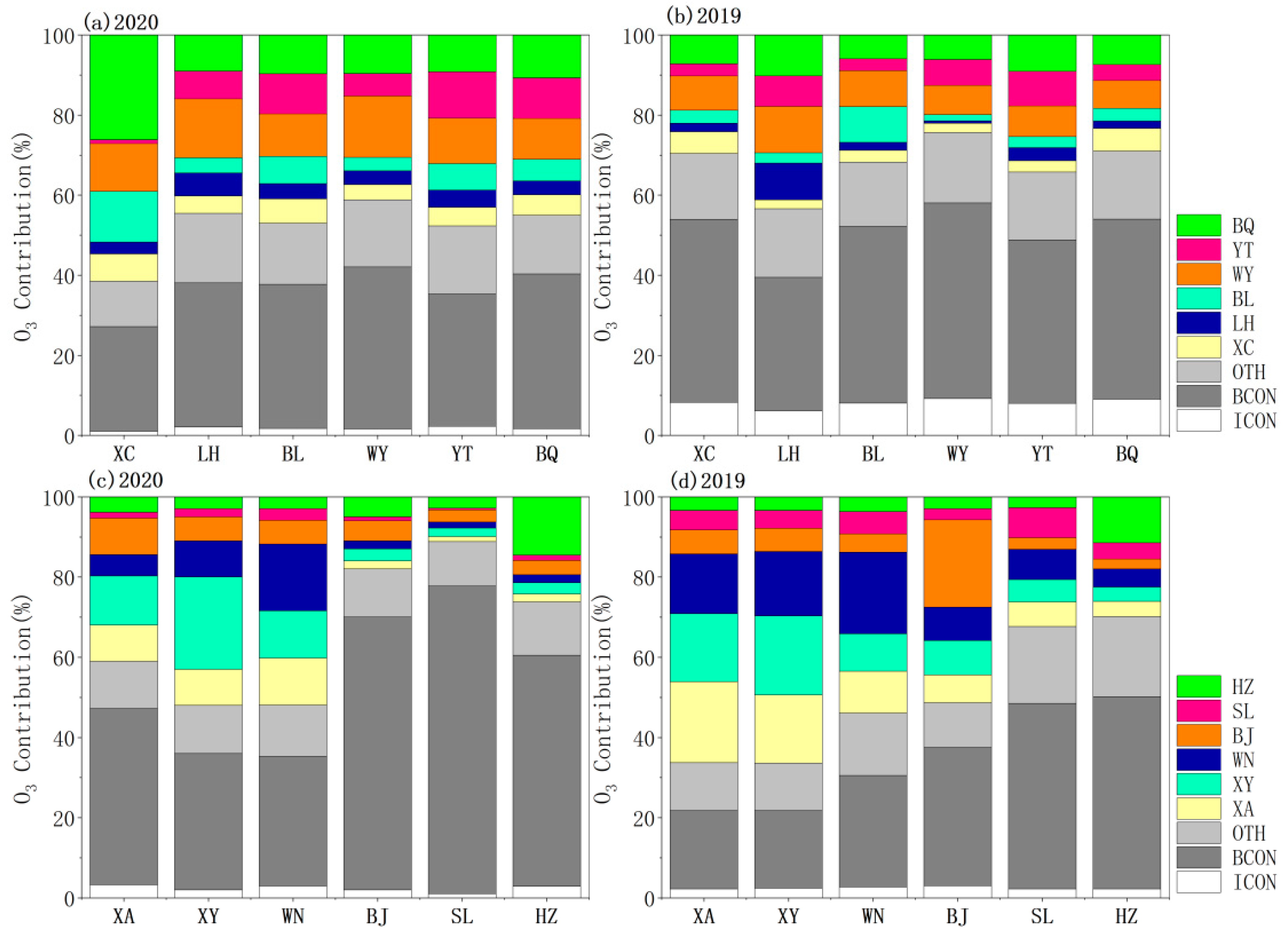
The O3 source resolution analysis was divided into the following two scenarios: (1) the labeling of all areas without distinguishing between emission source types, with each area containing all four source types; and (2) the labeling of each emission source type without differentiating the areas. Additionally, the initial conditions (ICONs), boundary conditions (BCONs), and default emission sources not explicitly labeled in the model (OTH) were automatically categorized as complementary contributions. BCONs primarily comprise global background values and long-range transport from sources outside a simulated region [45].
This study utilized three nested layers to investigate the causes of the increase in O3 concentrations in Xi’an during February 2020. The results from the d01 layer were used to assess contributions to the d02 and d03 layers, primarily representing external pollutant transport. The d02 layer’s ISAM setup examined the regional and industrial emission contributions from Xi’an and five neighboring cities to urban O3 concentrations in Xi’an. The d03 layer concentrated on the contributions from regional and industrial sources in neighboring cities to urban O3 levels in Xi’an. The ISAM settings in the d02 layer were also utilized to analyze the contributions from six major urban areas in Xi’an to O3 concentrations. All regions and industries were labeled and monitored, including ICONs, BCONs, and OTH, to identify their contributions to O3 levels in Xi’an. Table 4 presents detailed labeling information.

3.3.1. Contribution of BCONs

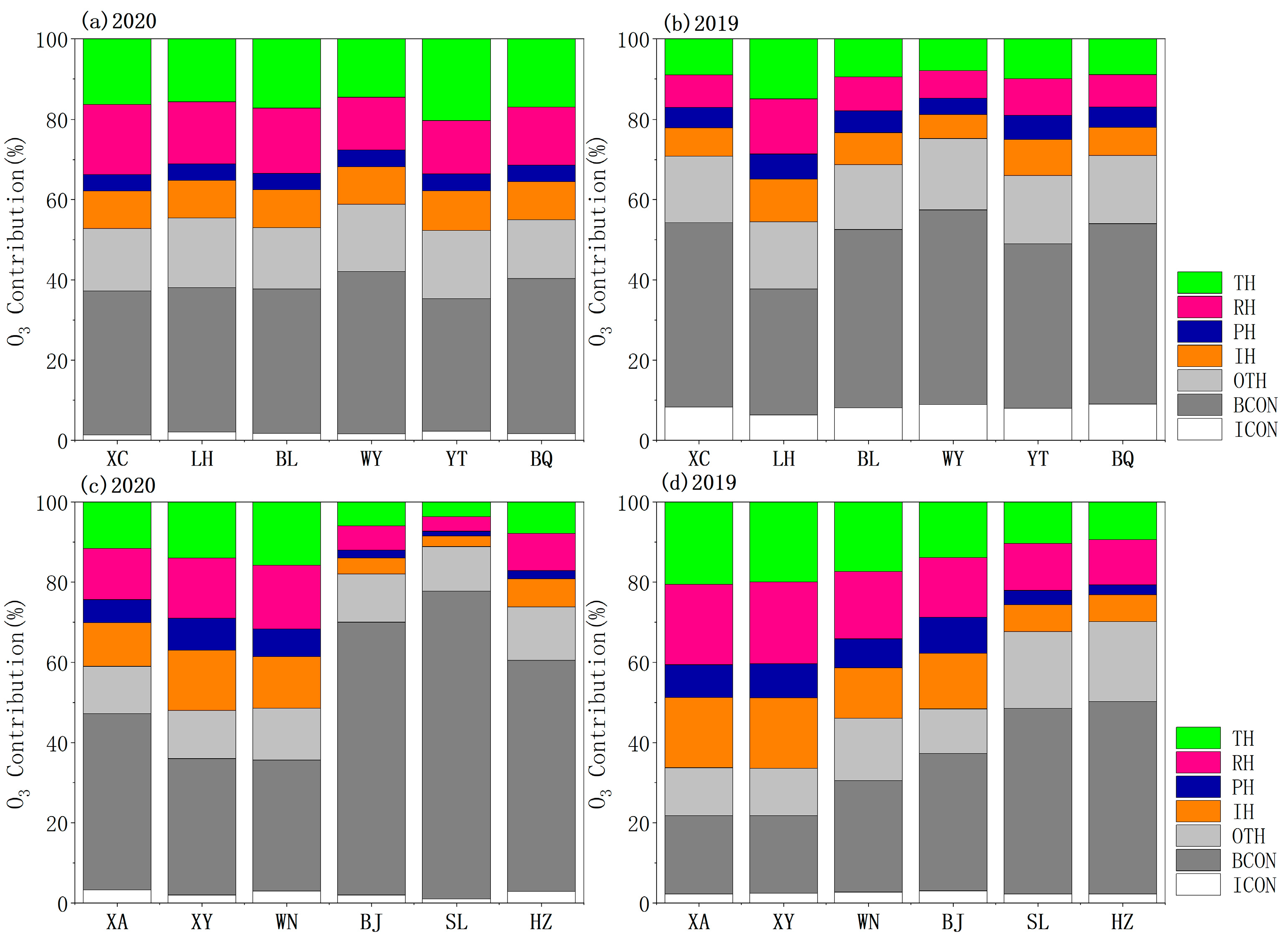
Figure 6 and Figure 7 illustrate that BCONs were the primary contributors to O3 concentrations, regardless of the consideration of regional or sectoral sources. In Xi’an’s major urban areas, the BCON contribution exceeded 30% in 2020, with WY recording the highest at 40.42% and YT the lowest at 33%. Similar trends were noted in 2019, with BCONs contributing 49% to WY, 45% to BQ, 45.71% to XC, and the lowest contribution of 33.38% to LH. In 2019, the BCON contribution to each urban area remained above 30%, which was higher than in 2020, with WY again recording the highest at 49%. In both 2019 and 2020, BCONs significantly contributed to O3 levels in Xi’an and the surrounding cities. SL exhibited the largest BCON contribution among all cities, reaching 76.71% in 2020, and similarly held the highest contribution in 2019. The BCON contribution to O3 levels in Xi’an and nearby cities was greater in 2020 than in 2019. In XA, the BCON contribution increased from 19.57% to 43.98%, indicating a significant rise in BCONs’ influence on Xi’an in 2020 compared with 2019. Detailed contributions of specific concentrations are provided in Tables S2–S9.
The analysis identified BCONs as the largest contributor to O3 concentrations. For instance, Liu et al. [43] found that BCONs accounted for 78% of the total simulated O3 concentration in the Beijing–Tianjin–Hebei region. Similarly, Collet et al. [39] observed that BCONs contributed over 50% to O3 concentrations in several U.S. cities, including Denver, Phoenix, Los Angeles, and Detroit. In Zhoushan city, Li et al. [46] reported that BCONs contributed over 60% to the total simulated O3 concentration at all sites. These findings suggest that long-distance transport significantly contributes to O3 levels and is a dominant source. This occurs because O3 formation requires time and can be transported over long distances by air masses. Additionally, Xi’an’s location in the western section of the Fenwei Plain—a Cenozoic fault basin formed by the Himalayan movement—further influences this process. The dominant wind direction in Xi’an is northeasterly, with annual static wind rates of 35% and 45% in winter. Mountain ranges and the sinking effect of airflow on leeward slopes create anticyclonic stagnation zones, where ground-level convergence hinders pollutant dispersion during pollution events [28]. Data from the Shanxi Provincial Meteorological Bureau indicate a significant decline in wind speeds in the Guanzhong area, averaging a decrease of 0.09 m/s per decade. The slower wind speeds and complex terrain impede pollutant dispersion, resulting in the accumulation of O3 and other pollutants. The following section discusses the impact of regional transport and industrial changes on rising O3 levels, focusing on contributions from surrounding cities to major urban areas.

3.3.2. O3 Source Apportionment of Regions in d02

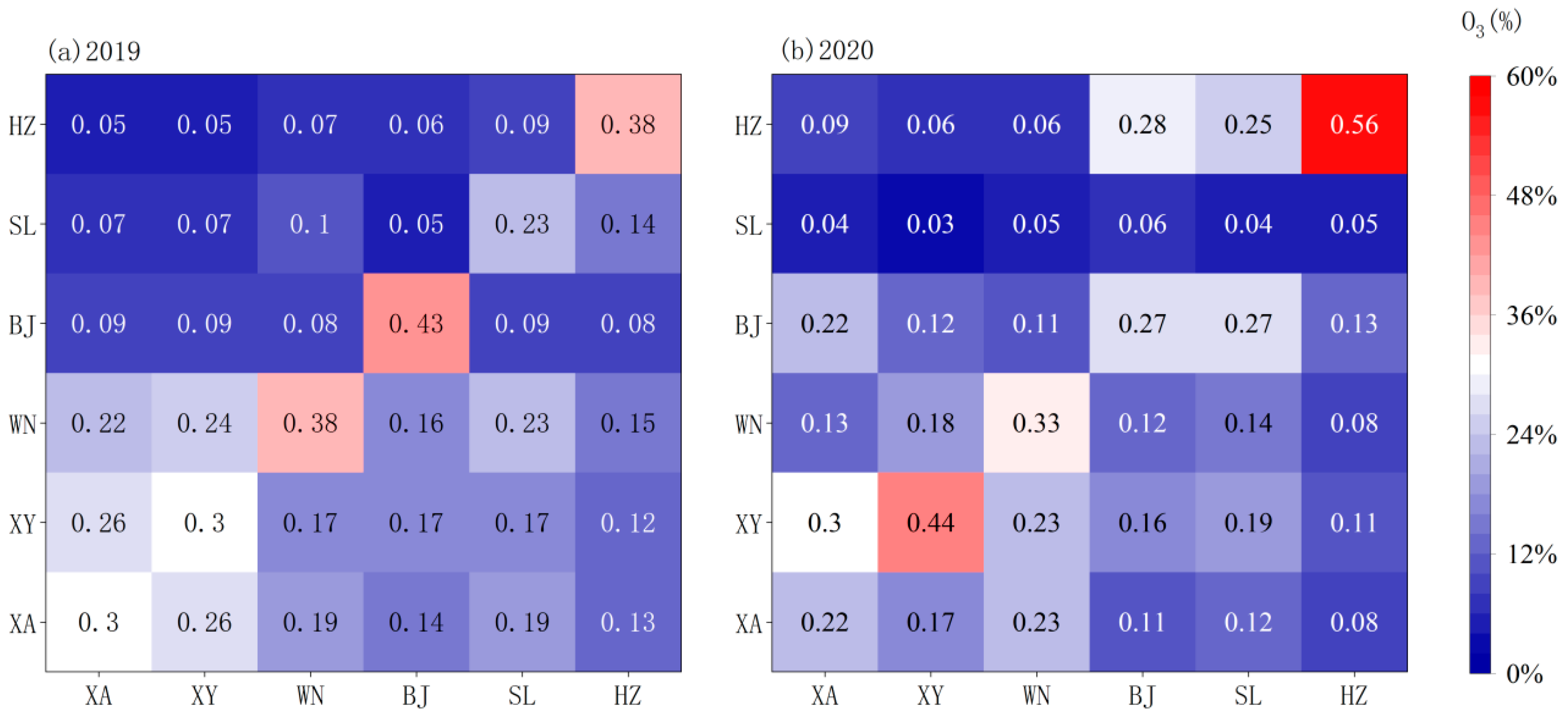
Figure 8 illustrates the contributions of O3 concentrations from d02, excluding XA and the BCONs, ICONs, and OTH of neighboring cities. The figure indicates that nearly every city significantly contributed to its own O3 levels. In 2019, the contributions to XA’s O3 concentrations, in descending order, were XA (30%), XY (26%), WN (22%), BJ (9%), SL (7%), and HZ (5%). In 2020, the contributions to XA’s O3 levels, in descending order, were XY (30%), XA (22%), BJ (22%), WN (13%), HZ (9%), and SL (4%). In 2020, XY was the largest contributor to XA’s O3 concentration, accounting for 30%, surpassing XA’s own contribution of 22%. BJ also contributed 22%, matching XA’s own contribution. Therefore, BJ’s contribution to XA’s O3 levels increased in 2020, while WN’s contribution decreased. Song et al. [15] noted that XA’s O3 pollution was primarily influenced by short-range airflow, with significant contributions from northward, southwesterly, and northeasterly flows. Overall, southwestern cities contributed less O3 to XA in both years due to the Qinling Mountains, which served as a barrier that hindered the diffusion of O3 from HZ and SL. In winter, prevailing northwesterly winds in Shaanxi Province transported pollutants from BJ and XY to XA, where they were obstructed by the Qinling Mountains. Additionally, XA’s static wind rate reached 40% in winter, increasing annually and contributing to O3 accumulation. This was consistent with the study of Yan et al. on O3 pollution in Guanzhong [47], which highlighted how the Qinling Mountains influence weather patterns and contribute to pollutant accumulation.

3.3.3. O3 Source Apportionment of Emissions in d02

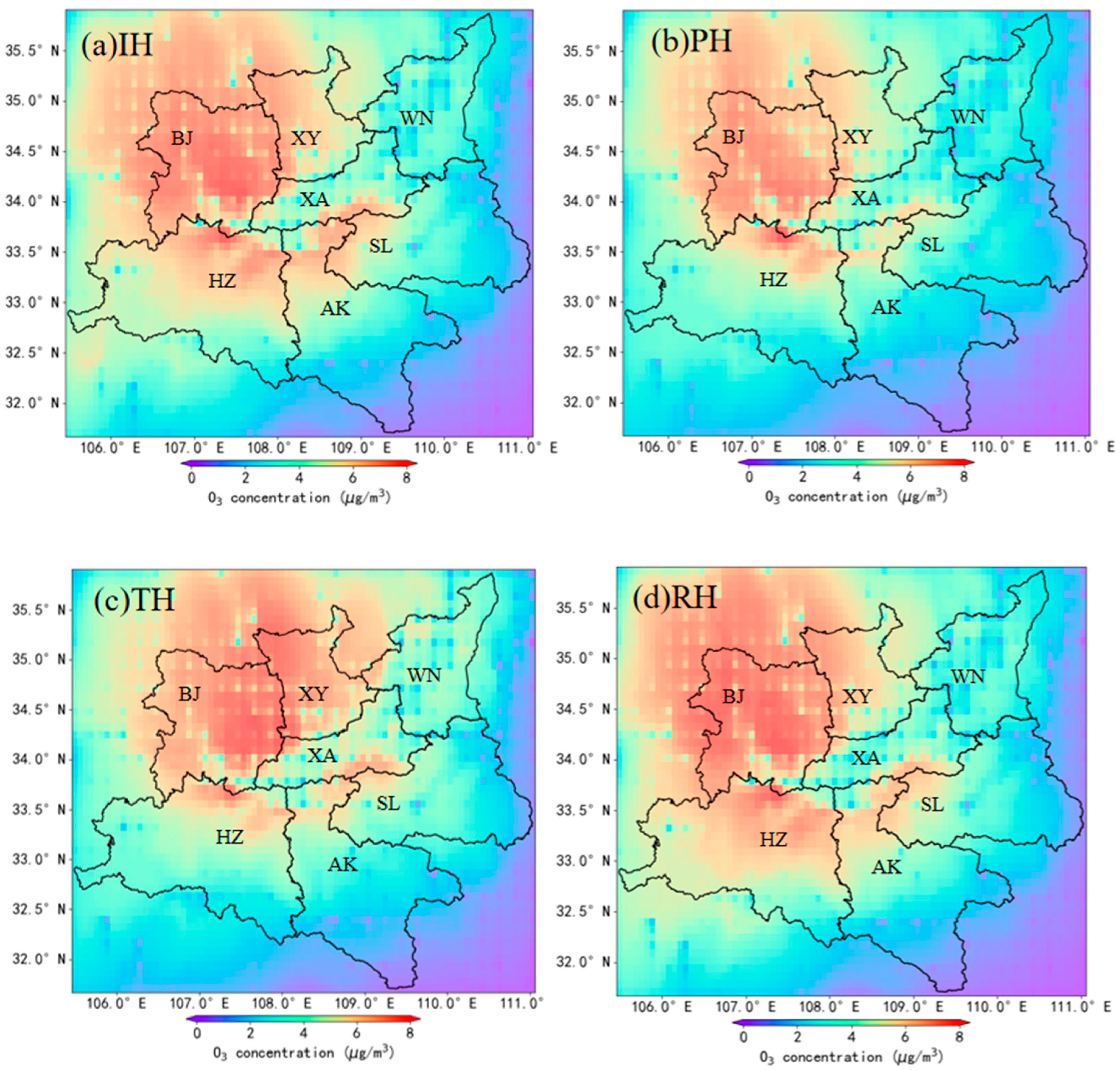
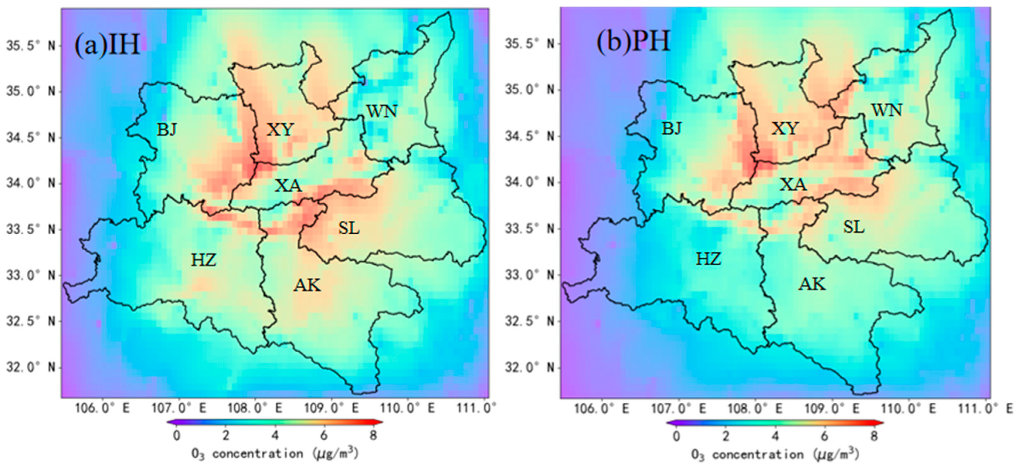
A comparison of industrial contributions to O3 in February 2020 and 2019, as shown in Tables S4 and S5, revealed minimal differences between the two years. The ranking of O3 contributions remained consistent, ordered as follows from largest to smallest: RH (28–38%), TH (27–33%), IH (21–28%), and PH (8–18%). Figure 9 and Figure 10 illustrate the contributions of industrial emissions to O3 concentrations in XA and the surrounding urban areas for February 2020 and 2019. Figure 10 (February 2019) shows that the peak O3 contributions from industries were evenly distributed around XA. However, by February 2020 (Figure 9), contributions from TH in BJ increased by 4%, RH by 5%, IH in XY by 2%, and PH by 3% compared with 2019, aligning with the findings in Section 3.3.2. The increased regional contributions from BJ and XY, as analyzed in Section 3.2, suggested that BJ’s O3 contribution to XA primarily arose from transportation and residential sources, while XY’s contribution mainly resulted from industrial and power sources. Ou et al. [48] noted that XY and XA are core cities in the Guanzhong region; BJ also demonstrates strong economic competitiveness within the urban cluster, particularly in transportation accessibility and economic development.

3.3.4. O3 Source Apportionment of Regions in d03

Figure 11 illustrates the O3 contributions from both local and regional transport to d03, including XA’s urban areas. Except for XC, each urban area predominantly contributed to its own O3 levels, confirming the conclusion in Section 3.3.3 that cities primarily influenced their own local O3 concentrations. BQ contributed slightly more to XC’s O3 levels than XC itself, likely because XC has a smaller urban area and is adjacent to the larger, more complex air mass of BQ, resulting in a greater impact from BQ. The heat map visually indicated that BQ, WY, and YT exerted the greatest influence on other urban areas, with their O3 contributions to these areas increasing in 2020. This phenomenon arose because XC, LH, and BL are densely populated urban centers where low O3 concentrations are common, as noted in the study of Zhang et al. [49]. O3 precursors primarily originate from urban traffic and industrial emissions. As O3 is a secondary pollutant, it requires time to form and is gradually removed from the air. A significant number of precursors from urban centers is transported downwind to suburban areas, where ample oxygen and sunlight create favorable conditions for O3 formation.

3.3.5. O3 Source Apportionment of Emissions in d03

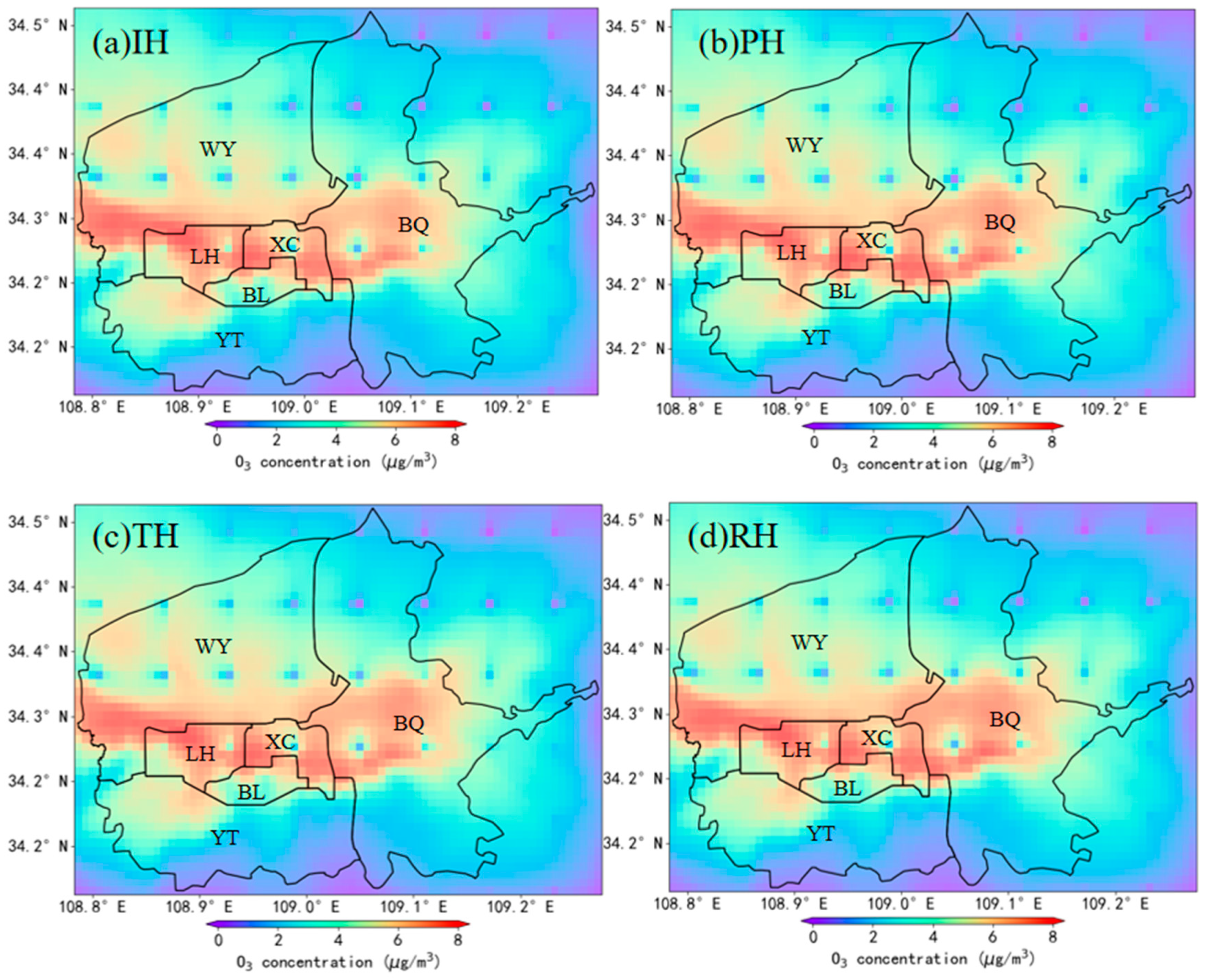
Figure 12 and Figure 13 illustrate the changes in industrial source contributions to O3 concentrations in d03 between February 2019 and February 2020. The figures demonstrate a clear trend of industrial source contributions to O3 concentrations spreading from the center to the periphery and toward the northwest. From February 2019 to February 2020, O3 contributions from IH and PH decreased across all urban areas, while those from RH and TH increased, with the most significant TH contribution occurring in WY, BQ, and YT. Consequently, WY, BQ, and YT experienced increased O3 contributions, driven by higher emissions from industrial sources, which explained the rise in O3 contributions in WY and BQ in 2020. The primary cause of the increased O3 concentrations in February 2020 was the rise in transportation emissions, followed by contributions from residential sources. Emissions of NOx from transportation are key precursors to O3 formation, significantly contributing to rises in O3 concentrations.

3.4. Discussion of Results

The source resolution of ozone in Section 3.3 enabled us to further investigate the causes behind the increase in ozone concentration observed in February 2020.
Firstly, the urban agglomeration in d02, serving as the boundary condition for d03, was the primary contributor to the rise in O3 levels in Xi’an, with BCONs increasing from 19.57% to 43.98%. Many studies using CMAQ-ISAM have highlighted the role of BCONs as a major contributor to O3. Xian et al. [50] found that during the warm season in Chengdu, BCONs accounted for 37.4% to 65.7% of O3 in various regions [49,51]. The source analysis of d02 indicated that this increase was primarily due to heightened contributions from local transportation and residential sources in XY and BJ. This led to an increased local O3 contribution in these areas. Yan et al. [47] also noted that ozone pollution in XY was exacerbated by significant contributions from traffic sources in the Guanzhong Plain during summer. Additionally, the dominant northwesterly winds in XA facilitated the transfer of locally generated O3 from XY and BJ. The increase in easterly airflow at high altitudes and the blockage by the Qinling Mountains caused O3 and its precursors to accumulate in downwind areas, resulting in elevated O3 concentrations in XA. These findings were consistent with related studies on the effects of weather circulation on O3 and its precursors. The increase in emissions from transportation sources in BQ, WY, and YT in 2020 compared with 2019 was a key factor in the rising local O3 contribution in the Xi’an metropolitan area. Song and Hao et al. [15] also noted a year-to-year increase in local O3 concentrations from 2014 to 2020, attributing this rise to significant contributions from heavy daytime traffic sources. Overall, the increase in O3 concentration in XA was primarily due to enhanced long-distance transmission from surrounding urban agglomerations. Therefore, controlling O3 levels in XA should focus on local transportation and residential sources while also addressing contributions from BJ and XY [46], both of which are upwind and significantly impactful. A synergistic control approach involving these regions and XA is essential [52,53,54].

4. Conclusions

This study systematically reproduced an elevated O3 concentration event in XA and its urban areas during February 2020 using the WRF-CMAQ model. The model evaluation demonstrated its ability to accurately capture both temporal and spatial variations in meteorological parameters and air-pollutant concentrations. The regional and industrial sources of XA (d02) and XA’s urban areas (d03) were analyzed using the CMAQ-ISAM module. The impacts of various source contributions on elevated O3 concentrations were discussed, and intrinsic links between regional and industrial sources were identified. The key findings are as follows.
BCONs were the largest contributor of source contributions to O3 levels. The primary regional sources were BJ and XY, influenced by northwesterly winds and the Qinling Mountains. Major contributors of industrial sources included RH and TH, which emitted NOx and VOCs from densely populated areas and transport activities, leading to higher O3 levels. In XA’s urban areas, BQ was the largest contributor of urban contributions, followed by WY and YT, closely linked to the area’s population density and auto motive industry. Regulatory measures should prioritize a reduction in precursor emissions from the residential and transportation sectors to meet O3 air-quality standards.
A limitation of our study was the lack of exploration of the mechanisms of O3 formation, which led to an insufficient investigation of the synergistic effects between O3 and its precursors (NOx and VOCs) in Xi’an. Additionally, the CMAQ model tends to underestimate peak O3 levels in urban areas, which can lead to an underestimation of the contribution from anthropogenic sources. Future research should aim to improve the model’s performance with data assimilation and the construction of emission inventories using a top-down approach to enhance the understanding of O3 formation and the spatial–temporal effects of pollution and precursor distributions on O3 concentrations.

Supplementary Materials

The following supporting information can be downloaded at: https://www.mdpi.com/article/10.3390/atmos15101208/s1, Table S1: List of the 15 individual air quality monitoring sites and the meteorological station; Table S2: Contribution rates of O3 to the tagged regions of d02 under the regional source apportionment scenario in 2020; Table S3: Contribution rates of O3 to the tagged regions of d02 under the regional source apportionment scenario in 2019; Table S4: Contribution rates of O3 to the tagged regions of d02 under the source apportionment scenario for different emission types in February 2020; Table S5: Contribution rates of O3 to the tagged regions of d02 under the source apportionment scenario for different emission types in February 2019; Table S6: Contribution rates of O3 to the tagged regions of d03 under the source apportionment scenario for different emission types in February 2020; Table S7: Contribution rates of O3 to the tagged regions of d03 under the source apportionment scenario for different emission types in February 2019; Table S8: Contribution rates of O3 to the tagged regions of d03 under the source apportionment scenario for different emission types in February 2020; Table S9: Contribution rates of O3 to the tagged regions of d03 under the source apportionment scenario for different emission types in February 2019.

Author Contributions

Conceptualization, Y.C. and J.W.; Data Curation, C.F. and Y.C.; Formal Analysis, Y.C. and S.Z.; Investigation, Y.C.; Methodology, Y.C., S.Z. and X.Z.; Supervision, C.F. and J.W.; Visualization, Y.C., S.Z. and X.Z.; Writing—Original Draft, Y.C.; Writing—Review and Editing, J.W. and C.F. All authors have read and agreed to the published version of the manuscript.

Funding

This research received no external funding.

Institutional Review Board Statement

Not applicable.

Informed Consent Statement

Not applicable.

Data Availability Statement

The original contributions presented in the study are included in the article/Supplementary Materials, further inquiries can be directed to the corresponding authors.

Conflicts of Interest

The authors declare that they have no known competing financial interests or personal relationships that could have appeared to influence the work reported in this paper.

References

  1. Lu, B.; Zhang, Z.; Jiang, J.; Meng, X.; Liu, C.; Herrmann, H.; Chen, J.; Xue, L.; Li, X. Unraveling the O3-NOX-VOCs Relationships Induced by Anomalous Ozone in Industrial Regions during COVID-19 in Shanghai. Atmos. Environ. 2023, 308, 119864. [Google Scholar] [CrossRef] [PubMed]
  2. Wang, S.; Niu, Y.; Zhang, H.; Zhao, Z.; Zhang, X. Metabolomic Alterations in Healthy Adults Traveling to Low-Pollution Areas: A Natural Experiment with Ozone Exposure. Sci. Total Environ. 2023, 897, 165501. [Google Scholar] [CrossRef] [PubMed]
  3. Seiwert, B.; Nihemaiti, M.; Troussier, M.; Weyrauch, S.; Reemtsma, T. Abiotic Oxidative Transformation of 6-PPD and 6-PPD Quinone from Tires and Occurrence of Their Products in Snow from Urban Roads and in Municipal Wastewater. Water Res. 2022, 212, 118122. [Google Scholar] [CrossRef] [PubMed]
  4. Agathokleous, E.; Feng, Z.; Oksanen, E.; Sicard, P.; Wang, Q.; Saitanis, C.J.; Araminiene, V.; Blande, J.D.; Hayes, F.; Calatayud, V.; et al. Ozone Affects Plant, Insect, and Soil Microbial Communities: A Threat to Terrestrial Ecosystems and Biodiversity. Sci. Adv. 2020, 6, eabc1176. [Google Scholar] [CrossRef]
  5. Mills, G.; Pleijel, H.; Malley, C.S.; Sinha, B.; Cooper, O.R.; Schultz, M.G.; Neufeld, H.S.; Simpson, D.; Sharps, K.; Feng, Z.; et al. Tropospheric Ozone Assessment Report: Present-Day Tropospheric Ozone Distribution and Trends Relevant to Vegetation. Elem.-Sci. Anthr. 2018, 6, 47. [Google Scholar] [CrossRef]
  6. Song, X.; Hao, Y. An Assessment of O3-Related Health Risks and Economic Losses in Typical Regions of China. Front. Public Health 2023, 11, 1194340. [Google Scholar] [CrossRef]
  7. Feng, Z.; Xu, Y.; Kobayashi, K.; Dai, L.; Zhang, T.; Agathokleous, E.; Calatayud, V.; Paoletti, E.; Mukherjee, A.; Agrawal, M.; et al. Ozone Pollution Threatens the Production of Major Staple Crops in East Asia. Nat. Food 2022, 3, 47–56. [Google Scholar] [CrossRef]
  8. Lyu, X.; Li, K.; Guo, H.; Morawska, L.; Zhou, B.; Zeren, Y.; Jiang, F.; Chen, C.; Goldstein, A.H.; Xu, X.; et al. A Synergistic Ozone-Climate Control to Address Emerging Ozone Pollution Challenges. One Earth 2023, 6, 964–977. [Google Scholar] [CrossRef]
  9. Chen, Z.; Xie, Y.; Liu, J.; Shen, L.; Cheng, X.; Han, H.; Yang, M.; Shen, Y.; Zhao, T.; Hu, J. Distinct Seasonality in Vertical Variations of Tropospheric Ozone over Coastal Regions of Southern China. Sci. Total Environ. 2023, 874, 162423. [Google Scholar] [CrossRef]
  10. Wang, Y.; Jiang, S.; Huang, L.; Lu, G.; Kasemsan, M.; Yaluk, E.A.; Liu, H.; Liao, J.; Bian, J.; Zhang, K.; et al. Differences between VOCs and NOx Transport Contributions, Their Impacts on O3, and Implications for O3 Pollution Mitigation Based on CMAQ Simulation over the Yangtze River Delta, China. Sci. Total Environ. 2023, 872, 162118. [Google Scholar] [CrossRef]
  11. Zhang, K.; de Leeuw, G.; Yang, Z.; Chen, X.; Jiao, J. The Impacts of the COVID-19 Lockdown on Air Quality in the Guanzhong Basin, China. Remote Sens. 2020, 12, 3042. [Google Scholar] [CrossRef]
  12. Yang, X.; Yang, T.; Lu, Y.; Jiang, M.; Zhang, S.; Shao, P.; Yuan, L.; Wang, C.; Wang, L. Assessment of Summertime Ozone Formation in the Sichuan Basin, Southwestern China. Front. Ecol. Evol. 2022, 10, 931662. [Google Scholar] [CrossRef]
  13. Yan, Y.; Shi, W.; Wang, C.; Chen, Y. Source Attribution and Process Analysis of Summertime Ozone Pollution in Guanzhong Basin, Northwestern China. Atmosphere 2023, 14, 1742. [Google Scholar] [CrossRef]
  14. Yang, X.; Wu, K.; Lu, Y.; Wang, S.; Qiao, Y.; Zhang, X.; Wang, Y.; Wang, H.; Liu, Z.; Liu, Y.; et al. Origin of Regional Springtime Ozone Episodes in the Sichuan Basin, China: Role of Synoptic Forcing and Regional Transport. Environ. Pollut. 2021, 278, 116845. [Google Scholar] [CrossRef]
  15. Song, X.; Hao, Y. Analysis of Ozone Pollution Characteristics and Transport Paths in Xi’an City. Sustainability 2022, 14, 16146. [Google Scholar] [CrossRef]
  16. Su, F.; Xu, Q.; Yin, S.; Wang, K.; Liu, G.; Wang, P.; Kang, M.; Zhang, R.; Ying, Q. Contributions of Local Emissions and Regional Background to Summertime Ozone in Central China. J. Environ. Manag. 2023, 338, 117778. [Google Scholar] [CrossRef]
  17. Xie, Q.; Tham, Y.J.; Yu, X.; Wang, Z.; Ling, Z.; Wang, X.; Guo, H.; Wang, T. Seasonal Variations of O3 Formation Mechanism and Atmospheric Photochemical Reactivity during Severe High O3 Pollution Episodes in the Pearl River Delta Region. Atmos. Environ. 2023, 309, 119918. [Google Scholar] [CrossRef]
  18. Cheng, Z.; Luo, L.; Wang, S.; Wang, Y.; Sharma, S.; Shimadera, H.; Wang, X.; Bressi, M.; de Miranda, R.M.; Jiang, J.; et al. Status and Characteristics of Ambient PM2.5 Pollution in Global Megacities. Environ. Int. 2016, 89–90, 212–221. [Google Scholar] [CrossRef]
  19. Zhang, J.; Kang, L.; Li, H.; Ballesteros-Perez, P.; Skitmore, M.; Zuo, J. The Impact of Environmental Regulations on Urban Green Innovation Efficiency: The Case of Xi’an. Sustain. Cities Soc. 2020, 57, 102123. [Google Scholar] [CrossRef]
  20. Feng, R.; Xu, H.; Wang, Z.; Gu, Y.; Liu, Z.; Zhang, H.; Zhang, T.; Wang, Q.; Zhang, Q.; Liu, S.; et al. Quantifying Air Pollutant Variations during COVID-19 Lockdown in a Capital City in Northwest China. Atmosphere 2021, 12, 788. [Google Scholar] [CrossRef]
  21. Han, L.; Zhao, J.; Gu, Z. Assessing Air Quality Changes in Heavily Polluted Cities during the COVID-19 Pandemic: A Case Study in Xi’an, China. Sustain. Cities Soc. 2021, 70, 102934. [Google Scholar] [CrossRef]
  22. Zhou, Q.; Yun, J.; Li, X.; Zhang, X.; Liu, B.; Zhang, S.; Zheng, X.; Yue, W.; Li, X.; Zhang, W. Vehicle Emissions in a Megacity of Xi’an in China: A Comprehensive Inventory, Air Quality Impact, and Policy Recommendation. Urban Clim. 2023, 52, 101740. [Google Scholar] [CrossRef]
  23. Sun, J.; Shen, Z.; Zhang, Y.; Zhang, Z.; Zhang, Q.; Zhang, T.; Niu, X.; Huang, Y.; Cui, L.; Xu, H.; et al. Urban VOC Profiles, Possible Sources, and Its Role in Ozone Formation for a Summer Campaign over Xi’an, China. Environ. Sci. Pollut. Res. 2019, 26, 27769–27782. [Google Scholar] [CrossRef] [PubMed]
  24. Wang, P.; Chen, K.; Zhu, S.; Wang, P.; Zhang, H. Severe Air Pollution Events Not Avoided by Reduced Anthropogenic Activities during COVID-19 Outbreak. Resour. Conserv. Recycl. 2020, 158, 104814. [Google Scholar] [CrossRef]
  25. Zhang, X.; Fan, Y.; Yu, W.; Wang, H.; Zhang, X. Variation of Particulate Matter and Its Correlation with Other Air Pollutants in Xi’an, China. Pol. J. Environ. Stud. 2021, 30, 3357–3364. [Google Scholar] [CrossRef]
  26. Chen, Q.; Sun, H.; Mu, Z.; Wang, Y.; Li, Y.; Zhang, L.; Wang, M.; Zhang, Z. Characteristics of Environmentally Persistent Free Radicals in PM2.5: Concentrations, Species and Sources in Xi’an, Northwestern China. Environ. Pollut. 2019, 247, 18–26. [Google Scholar] [CrossRef]
  27. Han, L.; Qi, Y. Characterization of Spatial and Temporal Variations in Air Pollutants and Identification of Health Risks in Xi’an, a Heavily Polluted City in China. Atmosphere 2024, 15, 716. [Google Scholar] [CrossRef]
  28. Elser, M.; Huang, R.-J.; Wolf, R.; Slowik, J.G.; Wang, Q.; Canonaco, F.; Li, G.; Bozzetti, C.; Daellenbach, K.R.; Huang, Y.; et al. New Insights into PM2.5 Chemical Composition and Sources in Two Major Cities in China during Extreme Haze Events Using Aerosol Mass Spectrometry. Atmos. Chem. Phys. 2016, 16, 3207–3225. [Google Scholar] [CrossRef]
  29. Wang, K.; Gao, C.; Wu, K.; Liu, K.; Wang, H.; Dan, M.; Ji, X.; Tong, Q. ISAT v2.0: An Integrated Tool for Nested-Domain Configurations and Model-Ready Emission Inventories for WRF-AQM. Geosci. Model Dev. 2023, 16, 1961–1973. [Google Scholar] [CrossRef]
  30. Rajeswari, J.R.; Srinivas, C.V.; Mohan, P.R.; Venkatraman, B. Impact of Boundary Layer Physics on Tropical Cyclone Simulations in the Bay of Bengal Using the WRF Model. Pure Appl. Geophys. 2020, 177, 5523–5550. [Google Scholar] [CrossRef]
  31. Ek, M.; Mitchell, K.; Lin, Y.; Rogers, E.; Grunmann, P.; Koren, V.; Gayno, G.; Tarpley, J. Implementation of Noah Land Surface Model Advances in the National Centers for Environmental Prediction Operational Mesoscale Eta Model. J. Geophys. Res.-Atmos. 2003, 108, 282. [Google Scholar] [CrossRef]
  32. Hong, S.; Dudhia, J.; Chen, S. A Revised Approach to Ice Microphysical Processes for the Bulk Parameterization of Clouds and Precipitation. Mon. Weather Rev. 2004, 132, 103–120. [Google Scholar] [CrossRef]
  33. Kain, J. The Kain-Fritsch Convective Parameterization: An Update. J. Appl. Meteorol. 2004, 43, 170–181. [Google Scholar] [CrossRef]
  34. Iacono, M.; Mlawer, E.; Clough, S.; Morcrette, J. Impact of an Improved Longwave Radiation Model, RRTM, on the Energy Budget and Thermodynamic Properties of the NCAR Community Climate Model, CCM3. J. Geophys. Res.-Atmos. 2000, 105, 14873–14890. [Google Scholar] [CrossRef]
  35. Ruiz-Arias, J.A.; Dudhia, J.; Santos-Alamillos, F.J.; Pozo-Vazquez, D. Surface Clear-Sky Shortwave Radiative Closure Intercomparisons in the Weather Research and Forecasting Model. J. Geophys. Res.-Atmos. 2013, 118, 9901–9913. [Google Scholar] [CrossRef]
  36. Sarwar, G.; Luecken, D.; Yarwood, G.; Whitten, G.Z.; Carter, W.P.L. Impact of an Updated Carbon Bond Mechanism on Predictions from the CMAQ Modeling System: Preliminary Assessment. J. Appl. Meteorol. Climatol. 2008, 47, 3–14. [Google Scholar] [CrossRef]
  37. Zheng, B.; Tong, D.; Li, M.; Liu, F.; Hong, C.; Geng, G.; Li, H.; Li, X.; Peng, L.; Qi, J.; et al. Trends in China’s Anthropogenic Emissions since 2010 as the Consequence of Clean Air Actions. Atmos. Chem. Phys. 2018, 18, 14095–14111. [Google Scholar] [CrossRef]
  38. Kwok, R.H.F.; Baker, K.R.; Napelenok, S.L.; Tonnesen, G.S. Photochemical Grid Model Implementation and Application of VOC, NOx, and O3 Source Apportionment. Geosci. Model Dev. 2015, 8, 99–114. [Google Scholar] [CrossRef]
  39. Collet, S.; Kidokoro, T.; Karamchandani, P.; Jung, J.; Shah, T. Future Year Ozone Source Attribution Modeling Study Using CMAQ-ISAM. J. Air Waste Manag. Assoc. 2018, 68, 1239–1247. [Google Scholar] [CrossRef]
  40. Cao, J.; Qiu, X.; Liu, Y.; Yan, X.; Gao, J.; Peng, L. Identifying the Dominant Driver of Elevated Surface Ozone Concentration in North China Plain during Summertime 2012–2017. Environ. Pollut. 2022, 300, 118912. [Google Scholar] [CrossRef]
  41. Emery, C.; Liu, Z.; Russell, A.G.; Odman, M.T.; Yarwood, G.; Kumar, N. Recommendations on Statistics and Benchmarks to Assess Photochemical Model Performance. J. Air Waste Manag. Assoc. 2017, 67, 582–598. [Google Scholar] [CrossRef] [PubMed]
  42. Boylan, J.W.; Russell, A.G. PM and Light Extinction Model Performance Metrics, Goals, and Criteria for Three-Dimensional Air Quality Models. Atmos. Environ. 2006, 40, 4946–4959. [Google Scholar] [CrossRef]
  43. Liu, H.; Zhang, M.; Han, X.; Li, J.; Chen, L. Episode Analysis of Regional Contributions to Tropospheric Ozone in Beijing Using a Regional Air Quality Model. Atmos. Environ. 2019, 199, 299–312. [Google Scholar] [CrossRef]
  44. Liu, Y.; Wang, T. Worsening Urban Ozone Pollution in China from 2013 to 2017-Part 2: The Effects of Emission Changes and Implications for Multi-Pollutant Control. Atmos. Chem. Phys. 2020, 20, 6323–6337. [Google Scholar] [CrossRef]
  45. Kitagawa, Y.K.L.; Pedruzzi, R.; Galvão, E.S.; De Araújo, I.B.; Alburquerque, T.T.D.A.; Kumar, P.; Nascimento, E.G.S.; Moreira, D.M. Source Apportionment Modelling of PM2.5 Using CMAQ-ISAM over a Tropical Coastal-Urban Area. Atmos. Pollut. Res. 2021, 12, 101250. [Google Scholar] [CrossRef]
  46. Li, W.; Tong, S.; Cao, J.; Su, H.; Zhang, W.; Wang, L.; Jia, C.; Zhang, X.; Wang, Z.; Chen, M.; et al. Comparative Observation of Atmospheric Nitrous Acid (HONO) in Xi’an and Xianyang Located in the GuanZhong Basin of Western China. Environ. Pollut. 2021, 289, 117679. [Google Scholar] [CrossRef]
  47. Yan, Y.; Wang, X.; Qu, K.; Li, X.; Shi, W.; Peng, Z.; Zhang, Y. Impacts of Synoptic Circulations on Summertime Ozone Pollution in Guanzhong Basin, Northwestern China. Atmos. Environ. 2021, 262, 118660. [Google Scholar] [CrossRef]
  48. Ou, Y.; Qian, Y.; Zen, J.; Li, X. Research on the Spatial Pattern of Traffic Accessibility and Economic Connection in Guanzhong Urban Agglomeration. In Proceedings of the International Conference on Smart Transportation and City Engineering, Chongqing, China, 26–28 October 2021; Li, Z., Cen, F., Eds.; SPIE: Bellingham, WA, USA, 2021; Volume 12050. [Google Scholar]
  49. Zhang, S.; Zhang, Z.; Li, Y.; Du, X.; Qu, L.; Tang, W.; Xu, J.; Meng, F. Formation Processes and Source Contributions of Ground-level Ozone in Urban and Suburban Beijing Using the WRF-CMAQ Modelling System. J. Environ. Sci. 2023, 127, 753–766. [Google Scholar] [CrossRef]
  50. Xian, Y.; Zhang, Y.; Liu, Z.; Wang, H.; Wang, J.; Tang, C. Source Apportionment and Formation of Warm Season Ozone Pollution in Chengdu Based on CMAQ-ISAM. Urban Clim. 2024, 56, 102017. [Google Scholar] [CrossRef]
  51. Zhao, Y.; Li, Y.; Kumar, A.; Ying, Q.; Vandenberghe, F.; Kleeman, M.J. Separately Resolving NOx and VOC Contributions to Ozone Formation. Atmos. Environ. 2022, 285, 119224. [Google Scholar] [CrossRef]
  52. Meng, B.; Zhang, J.; Zhang, X. Detecting the Spatial Network Structure of the Guanzhong Plain Urban Agglomeration, China: A Multi-Dimensional Element Flow Perspective. Land 2023, 12, 563. [Google Scholar] [CrossRef]
  53. Shi, J.; Liu, S.; Qu, Y.; Zhang, T.; Dai, W.; Zhang, P.; Li, R.; Zhu, C.; Cao, J. Variations of the Urban PM2.5 Chemical Components and Corresponding Light Extinction for Three Heating Seasons in the Guanzhong Plain, China. J. Environ. Manag. 2023, 327, 116821. [Google Scholar] [CrossRef] [PubMed]
  54. Zhao, H.; Niu, Z.; Feng, X. Factors Influencing Improvements in Air Quality in Guanzhong Cities of China, and Variations Therein for 2014–2020. Urban Clim. 2021, 38, 100877. [Google Scholar] [CrossRef]
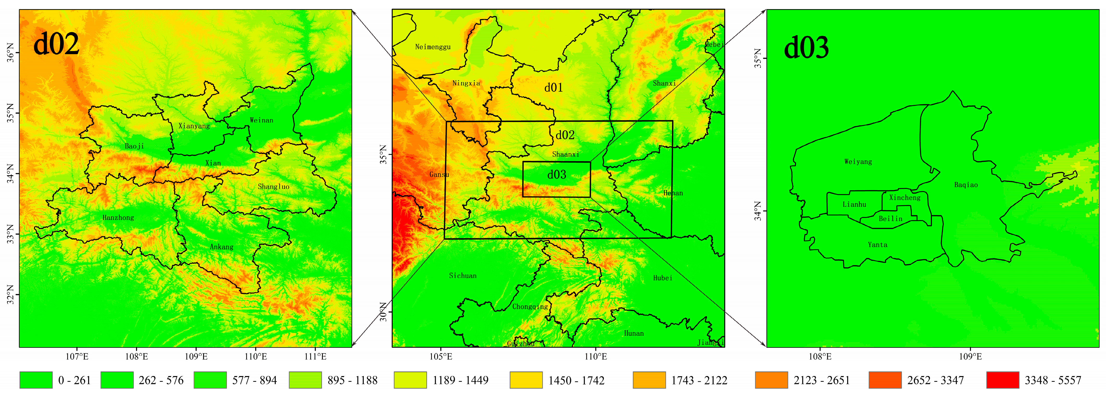
Figure 1. Map showing the triple-nested simulation domains, urban areas, and topography for each nest.
Atmosphere 15 01208 g001
Figure 2. Daily mean O3 concentrations in February 2020 (red line) vs. February 2019 (black line), February 2021 (blue line), February 2022 (green line), and average O3 concentrations for each month (dashed line).
Atmosphere 15 01208 g002
Figure 3. Comparison of temperature time series of meteorological stations in Xi’an.
Atmosphere 15 01208 g003
Figure 4. Comparison of wind-speed time series of meteorological stations in Xi’an.
Atmosphere 15 01208 g004
Figure 5. Comparison of O3-concentration time series in Xi’an.
Atmosphere 15 01208 g005
Figure 6. Contribution rates of O3 to the 12 tagged regions under the regional source apportionment scenario. (a,b) are the contribution of each tagged region in d02 to O3 in 2020 vs. in 2019, (c,d) are the contribution of each tagged region in d03 to O3 in 2020 vs. in 2019.
Atmosphere 15 01208 g006
Figure 7. Contribution rates of O3 to the 12 tagged regions under the source apportionment scenario for different emission types. (a,b) are the contribution of each tagged region in d02 to O3 in 2020 vs. in 2019, (c,d) are the contribution of each tagged region in d03 to O3 in 2020 vs. in 2019.
Atmosphere 15 01208 g007
Figure 8. Contribution rates of O3 to the tagged regions of d02 under the regional source apportionment scenario in 2019 (a) and 2020 (b).
Atmosphere 15 01208 g008
Figure 9. Contribution rates of O3 to the tagged regions of d02 under the source apportionment scenario for different emission types in February 2020: (a) IH; (b) PH; (c) TH; (d) RH.
Atmosphere 15 01208 g009
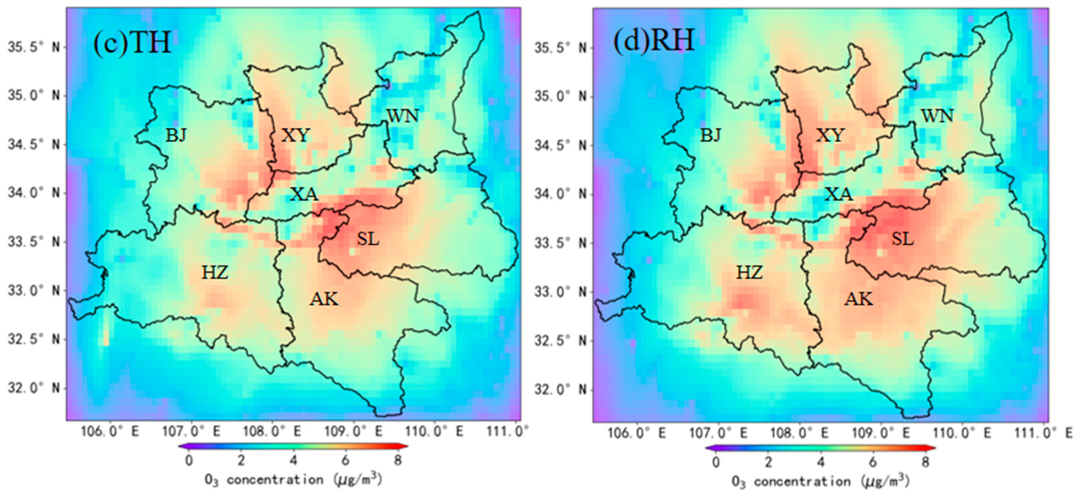
Figure 10. Contribution rates of O3 to the tagged regions of d02 under the source apportionment scenario for different emission types in February 2019: (a) IH; (b) PH; (c) TH; (d) RH.
Atmosphere 15 01208 g010aAtmosphere 15 01208 g010b
Figure 11. Contribution rates of O3 to the tagged regions of d03 under the regional source apportionment scenario in 2019 (a) and 2020 (b).
Atmosphere 15 01208 g011
Figure 12. Contribution rates of O3 to the tagged regions of d03 under the source apportionment scenario for different emission types in February 2020: (a) IH; (b) PH; (c) TH; (d) RH.
Atmosphere 15 01208 g012
Figure 13. Contribution rates of O3 to the tagged regions of d03 under the source apportionment scenario for different emission types in February 2019: (a) IH; (b) PH; (c) TH; (d) RH.
Atmosphere 15 01208 g013
Table 1. WRF and CMAQ modeling configurations.
ModelModel AttributionConfiguration
WRFPBL physics schemeYSU [30]
Surface-layer physicsMonin–Obukhov
Land-surface modelNoah [31]
MicrophysicsWSM6 [32]
Cumulus parameterizationKain–Fritsch [33]
Longwave radiationRRTM [34]
Shortwave radiationDudhia [35]
CMAQGas-phase chemistryCB05 [36]
Table 2. WRF simulation validation assessment.
MonthFactorNMBNMEIOAR
February 2019T2 (°C)34.23%37.47%0.960.97
WS10 (m/s)26.15%52.30%0.740.60
February 2020T2 (°C)5.83%38.96%0.910.76
WS10 (m/s)36.32%57.35%0.730.61
Table 3. Evaluation of CMAQ simulation effects.
MonthPollutantMFBMFEIOAR
February 2019O3−3.675%55.63%0.790.67
February 2020O311.64%47.85%0.620.43
Table 4. ISAM tagging information.
Tag TypeO3
Tagged regions (d03)Xincheng District (XC), Lianhu District (LH), Weiyang District (WY), Beilin District (BL), Baqiao District (BQ), and Yanta District (YT)
Tagged regions (d02)Xi’an city (XA), Xiyang city (XY), Weinan city (WN), Baoji city (BJ), Shangluo city (SL), and Hanzhong city (HZ)
Tagged industriesIndustrial (IH), power (PH), residential (RH), and transportation (TH)
Tagged source itemsInitial conditions (ICONs), boundary conditions (BCONs), and default emission sources not explicitly labeled in the model (OTH)
Disclaimer/Publisher’s Note: The statements, opinions and data contained in all publications are solely those of the individual author(s) and contributor(s) and not of MDPI and/or the editor(s). MDPI and/or the editor(s) disclaim responsibility for any injury to people or property resulting from any ideas, methods, instructions or products referred to in the content.