Article

Hydrometeorological Insights into the Forecasting Performance of Multi-Source Weather over a Typical Hill-Karst Basin, Southwest China

1
Key Laboratory of Disaster Prevention and Structural Safety of the Ministry of Education, Nanning 530004, China
2
College of Architecture and Civil Engineering, Guangxi University, Nanning 530004, China
3
Guangxi Provincial Engineering Research Center of Water Security and Intelligent Control for Karst Region, Guangxi University, Nanning 530004, China
4
Guangxi Key Laboratory of Disaster Prevention and Engineering Safety, Guangxi University, Nanning 530004, China
5
Shanghai Nuclear Engineering Research & Design Institute Co., Ltd., Shanghai 310000, China
6
Guangxi Water & Power Design Institute Co., Ltd., Nanning 530023, China
*
Author to whom correspondence should be addressed.
Atmosphere 2024, 15(2), 236; https://doi.org/10.3390/atmos15020236
Submission received: 2 January 2024 / Revised: 30 January 2024 / Accepted: 13 February 2024 / Published: 17 February 2024
(This article belongs to the Section Meteorology)

Abstract

:
Reliable precipitation forecasts are essential for weather-related disaster prevention and water resource management. Multi-source weather (MSWX), a recently released ensemble meteorological dataset, has provided new opportunities with open access, fine horizontal resolution (0.1°), and a lead time of up to seven months. However, few studies have comprehensively evaluated the performance of MSWX in terms of precipitation forecasting and hydrological modeling, particularly in hill-karst basins. The key concerns and challenges are how precipitation prediction performance relates to elevation and how to evaluate the hydrologic performance of MSWX in hill-karst regions with complex geographic heterogeneity. To address these concerns and challenges, this study presents a comprehensive evaluation of MSWX at the Chengbi River Basin (Southwest China) based on multiple statistical metrics, the Soil and Water Assessment Tool (SWAT), and a multi-site calibration strategy. The results show that all ensemble members of MSWX overestimated the number of precipitation events and tended to have lower accuracies at higher altitudes. Meanwhile, the error did not significantly increase with the increased lead time. The “00” member exhibited the best performance among the MSWX members. In addition, the multi-site calibration-enhanced SWAT had reliable performance (Average Nash–Sutcliffe value = 0.73) and hence can be used for hydrological evaluation of MSWX. Furthermore, MSWX achieved satisfactory performance (Nash–Sutcliffe value > 0) in 22% of runoff event predictions, but the error increased with longer lead times. This study gives some new hydrometeorological insights into the performance of MSWX, which can provide feedback on its development and applications.

1. Introduction

Reliable seasonal precipitation forecasts are essential for weather-related disaster control, reservoir scheduling, and water allocation decisions [1]. The widely used forecasting products include the Beijing climate center-climate prediction system (BCC-CPS) [2], the new ECMWF seasonal forecast systems (SEAS5) [3], the Met Office fully coupled atmosphere–ocean Global Seasonal Forecast System 5 (GloSea5) [4], the National Centers for Environmental Prediction Climate Forecast System (NCEP-CFS) [5], and the Bureau of Meteorology’s coupled model seasonal forecast system (POAMA) [6]. These products typically use partial differential formulations to describe atmospheric states and then apply numerical approximations to solve for the states at a specific resolution. Meanwhile, these products have provided valuable seasonal precipitation forecasts to support various applications, including those related to agriculture [7], hydrology [8], and the environment [9].
However, there is high uncertainty in these forecast products owing to the model’s parameters, initial conditions, and spatial scale [10]. For example, the friction force is typically neglected in parameterization schemes [11]. The SEAS5 and NCEP-CFS systems use ERA5 and GDAS assimilation data as initial states, respectively; nevertheless, these assimilated data are inherently subject to error, especially in regions with complex topography [12,13]. In addition, all forecast products fail to provide sub-grid-scale information due to grid-based solution strategies. Therefore, several studies have attempted to evaluate those products to support their development and application. For example, Wang et al. [14] found that SEAS5 offers considerable average performance in precipitation forecasting. However, the performance exhibits significant spatial variability, especially in mountainous watersheds. Hudson et al. [15] revealed that POAMA is performing relatively satisfactorily in eastern and southeastern Australia, but there is still much room for improvement elsewhere. Wu et al. [16] found that post-processing methods are effective in minimizing SEAS5 errors and reducing application uncertainty. Scaife et al. [2] found that some forecasting systems have relatively poor performance in the East Pacific due to inadequate capture of ENSO variability. White et al. [17] found that the imprecise representation of coupled atmosphere-ocean interactions in the climate prediction systems left them with some persistent biases. These studies have strengthened our understanding of precipitation forecasting products and highlighted (among other things) the sophistication of the SEAS5 system and, thus, its relative superiority for precipitation forecasting [3]; the high uncertainty of precipitation forecasts in complex terrain and, therefore, the importance of performance evaluation to feedback on algorithm development [18]; and the coarse spatial resolution (≥0.25°) of the aforementioned products and, hence, the limited capacity in mountainous regions [19].
As an effort to obtain more fine-scale forecasts, the multi-source weather (MSWX) dataset was released in 2022 with support from the European Research Council [20]. Specifically, the dataset consists of four sub-products, of which the Long sub-product is constructed based on SEAS5 product. Compared to SEAS5, the MSWX has an enhanced spatial resolution (0.1°) and, thence, an improved performance for capturing precipitation heterogeneity [20]. Meanwhile, cumulative distribution correction is used in MSWX to reduce the systematic bias of the SEAS5. Consequently, multi-source weather provides new opportunities in regions with complex terrain and precipitation systems. However, there are limited studies that have evaluated the accuracy of MSWX [21]. In addition, the hydrological performance of MSWX remains unexplored in complex topographic regions, such as mountainous watersheds and Karst-dominated basins.
With the development of computer technology and the advancement of the hydrological community, semi-distributed hydrological models have been proposed and are emerging as powerful tools for hydrological modeling [22]. Meanwhile, sub-basin delineation and geography-based parameters are used in semi-distributed hydrological models to mimic geospatial heterogeneity. Some of the widely used semi-distributed models include the Grid-Xinanjiang model [23], soil and water assessment tool (SWAT) [24,25], variable infiltration capacity [26], and topography-based hydrological model [27]. Amongst these models, the SWAT is a powerful open-source hydrological model with long-term simulation capabilities, spatial flexibility, and process-based modeling. It is continuously developed and improved by researchers worldwide, and thus its reliability has been widely verified [28]. More importantly, the foundational climate, soil, and topographic data for SWAT are available from open-access databases, including Geospatial Data Cloud, GDEMV2, GlobeLand30 [29], and Harmonized World Soil Database [30]. Therefore, the SWAT model is easily implemented in any terrain, including plain and mountain watersheds.
Mountainous terrain and karst landscapes are common geographic features around the globe, especially in southern China and Europe [31,32]. Under the effect of karst geology, these regions have a relatively low capacity for water retention, rendering them very vulnerable to weather-related disasters [33]. Meanwhile, the spatial heterogeneity of precipitation in these areas is significant owing to the influence of topography. However, precipitation forecasts based on partial differential formulations and numerical approximations may be unreliable due to the complex climate systems in mountain regions [34]. The precipitation heterogeneity also poses a great challenge to the effectiveness of precipitation forecasts. Therefore, there is an urgent need to evaluate the performance of MSWX in hill-karst regions to support its development and application.
The main objective of this study is to comprehensively evaluate the performance of MSWX in terms of precipitation forecasting and hydrological modeling over a hill-karst basin. The key concerns and challenges are how precipitation prediction performance relates to elevation and how to evaluate the hydrologic performance of MSWX in hill-karst regions with complex geographic heterogeneity. Connected to the main objective and challenges, this study can be further subdivided into the following: (1) to evaluate the accuracy of MSWX at various lead times using gauge precipitation observations as a reference; (2) to develop a SWAT model using a multi-site calibration strategy to account for geographic heterogeneity; and (3) to assess the hydrological performance of MSWX in runoff forecasting based on various statistical metrics. The structure chart of this study is shown in Figure 1.

2. Study Basin and Data

2.1. Study Basin

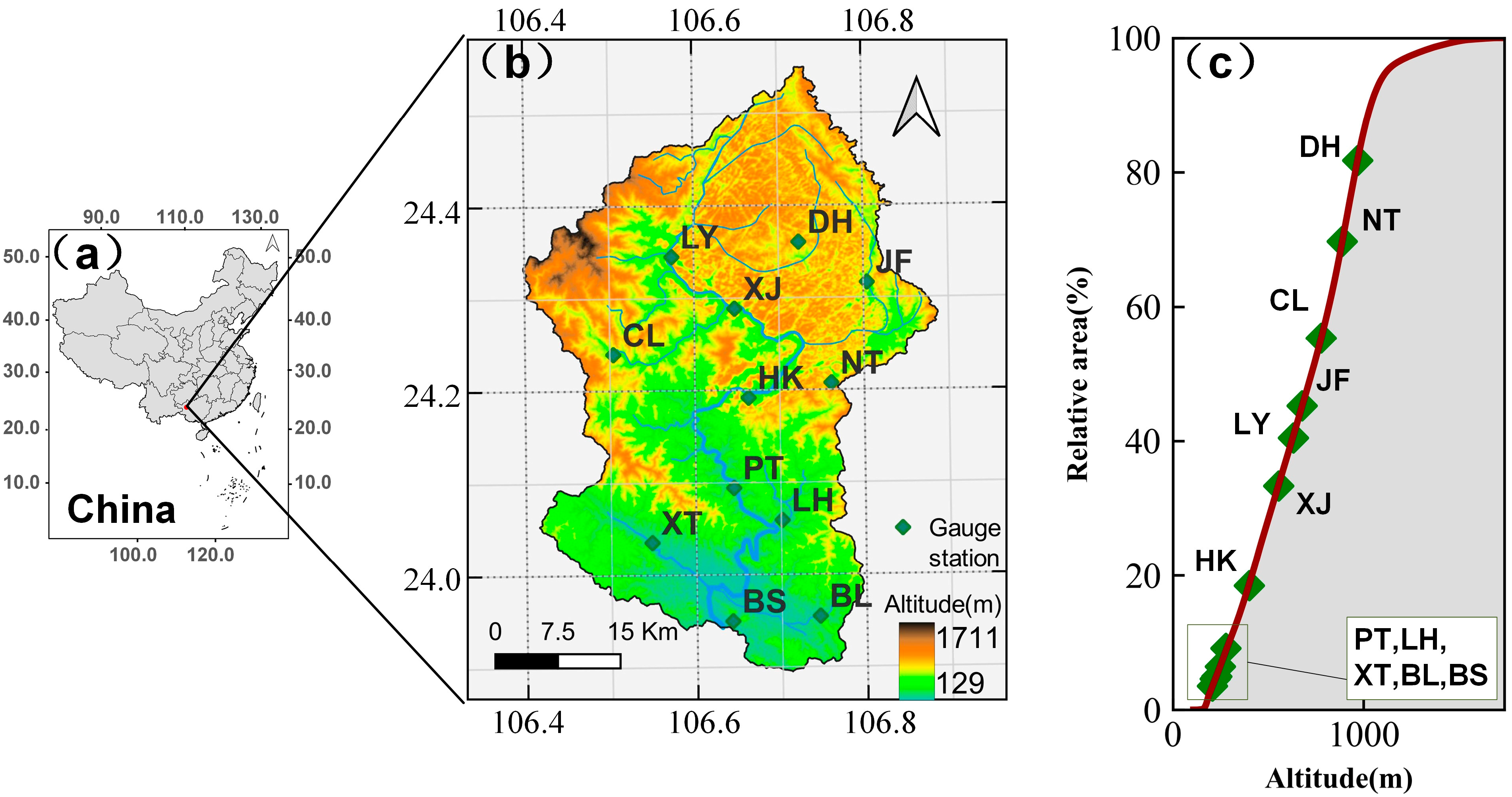
Chengbi River (CR) Basin is located in Guangxi, southwest China (Figure 2). The total area of the basin is 2087 km2, of which the karst area is about 1123 km2. Meanwhile, the total length of the river in the basin is 151 km, and the main stream originates from the northern foot of Qinglong Mountain, with a total drop of the river channel of 491 m. The spatial and elevational distribution of hydrometeorological stations is shown in Figure 2b and Figure 2c, respectively. Although some of those stations are located in the low latitude zone (elevation < 500), others are relatively evenly distributed across the hypsometric curve of CR Basin (Figure 2c). Meanwhile, the spatial distribution of stations is relatively uniform (Figure 2b). In addition, the density of stations in the watershed is about 174 km2/gauge, which is better than the WMO regulation for mountainous areas (250 km2/gauge) [35]. Therefore, these hydrometeorological stations provide a good representation of regional precipitation. However, under the combined effect of mountainous terrain and karst geomorphology, the Chengbi River Basin is highly susceptible to hydrometeorological-related disasters [33]. Meanwhile, there is a large reservoir located downstream of the outlet of the CR basin, and the reservoir has the functions of power generation, flood control, irrigation, and water supply. Therefore, reliable precipitation forecasts are essential for local weather-related disaster control and reservoir scheduling decisions.

2.2. Precipitation and Runoff Observations

Currently, there are twelve hydrometeorological stations within the CR basin, of which nine are precipitation stations (measuring only the precipitation element) and three are hydrologic stations (measuring both precipitation and runoff elements) (Figure 2). The precipitation observations used in this study consisted of daily precipitation recorded using an automated meteorological gauge (CAWS600) at 12 stations (Figure 2b and Table 1). The data source is the Chengbi River Reservoir Bureau, and the data quality was strictly controlled before acquisition [36]. In this study, daily gauge precipitation from 2002 to 2019 was collected for hydrologic modeling and MSWX evaluation. In addition, the daily runoff measured by PT, XJ, and BS stations from 2002–2019 was collected for hydrologic model calibration and validation. It should be noted that the XJ station no longer measures runoff elements after 2017. The runoff data from 2002–2010 was used for model calibration while that from 2011–2019 was applied for model validation. Finally, the daily runoff from 2011~2019 at the outlet of the CR basin (BS station) was used as a reference to evaluate the hydrological performance of MSWX in runoff forecasting. The approximate information of these hydrometeorological stations in CR Basin is shown in Table 1.

2.3. Multi-Source Weather (MSWX)

MSWX dataset is a global-scale high-resolution meteorological product, which was released in March 2022 with continuous updates [20]. The dataset consists of four sub-products: (i) Past subproduct, covering 1 January 1979 to ~5 days from real-time; (ii) NRT subproduct, covering extension to ~3 h from real-time; (iii) Mid subproduct, 10-day forecast ensemble comprising 30 members; and (ii) Long subproduct, covering 7-month forecast ensemble. The Long subproduct evaluated in this study is constructed based on the downscaling and bias correction of the SEAS5 product, and the subproduct has an enhanced spatial resolution of 0.1° and a temporal resolution of 1 d. Specifically, SEAS5 outputs are resampled from 1° to 0.1° resolution using nearest neighbor interpolation. Subsequently, a CDF-matching approach is used to reduce the bias of the resampled data [19]. In addition, MSWX historical retrospective forecasts were made with 1 January, 1 April, 1 July, and 1 October of each year between 1993 and 2020 as a starting point. Meanwhile, these retrospective forecasts include five members (MSWX 00-04), which are available for download from the official website (http://www.gloh2o.org/mswx/; last accessed on 23 October 2022). MSWX members have a nomenclature consistent with SEAS5. For example, MSWX 00 refers to the precipitation forecast based on SEAS5 00. The characteristics of MSWX members are summarized in Table 2.
In this study, the long sub-product of MSWX (version 100) from 2014 to 2019 with up to 90-day lead time was collected. Subsequently, we extracted gridded precipitation forecasts for 12 station locations (Figure 2b). Finally, the performance of the MSWX forecasts was evaluated using the station observations as a reference. In particular, the evaluation involved five MSWX members (i.e., MSWX 00-04), 12 grids corresponding to stations (see Figure 2b), six years (i.e., 2014–2019), four starting points (i.e., 1st day of January, April, July, and October), and up to 90 days of daily precipitation forecasts.

3. Methodology

3.1. Quantitative Metrics to Measure the Accuracy of MSWX in Precipitation Forecasting

The performance of precipitation prediction products is typically categorized into precipitation event (precipitation/non-precipitation) detection efficiency and intensity forecast capability [37]. In this study, probability of detection (POD), false alarm ratio (FAR), and critical success index (CSI) were used to evaluate the detection efficiency of MSWX. Meanwhile, Pearson’s correlation coefficient (Corr), Bias, and root mean square error (RMSE) were applied to evaluate the intensity forecast capability. These metrics were adopted because of their domain generalization and ease of understanding [37,38,39]. The formulas of these metrics are summarized in Table 3.

3.2. SWAT Hydrological Model and Its Calibration

A typical hydrological feature of hill-karst watersheds is their spatial heterogeneity. Therefore, the soil and water assessment tool (SWAT), a semi-distributed hydrological model, was used in this study to simulate hydrological processes. Specifically, the SWAT model is a basin-scale hydrologic tool with strong hydro-physical mechanisms [41]. It is based on multiple hydrologic response units to simulate hydrological processes, including evapotranspiration, infiltration, mid-soil flow, and surface and subsurface runoff. Therefore, the SWAT model can capture the spatial heterogeneity of hydrological processes. SWAT has been widely used in hydrological simulation owing to its high efficiency, ease of operation, fine performance, and continuous long-term simulation [42,43,44]. The principle of the SWAT model is to divide the watershed into several sub-watersheds. Subsequently, those sub-watersheds are further divided into various Hydrologic Response Units (HRU). Finally, hydrologic processes are simulated within each HRU. A detailed SWAT description is given in references [24,25]. The mathematical basis for the hydrological simulation of HRUs in the SWAT model is the water balance equation, which can be formulated as follows:
S W t = S W 0 + i = 1 t P day   , i Q s u f , i E a , i W s e p , i Q g w , i
where S W 0 and S W t denote the initial and final soil water content, respectively; P d a y , Q s u f , E a , W s e p , Q g w denote the daily precipitation, surface runoff, evapotranspiration, seepage flow, and sub-surface runoff, respectively, and the subscript i denotes a step; t denotes the simulation time. The units for all variables (except for subscripts) are millimeters.
Digital elevation, land use, and soil type are needed as foundational data in SWAT development and sub-basin delineation. In this study, digital elevation with a 30 m resolution was downloaded from Geospatial Data Cloud (https://www.gscloud.cn/), land use with a 30 m resolution was downloaded from (http://www.globallandcover.com/), soil type with a 1 km resolution was downloaded from (https://www.fao.org/soils-portal/). The meteorological data, including daily maximum and minimum temperatures, wind speed, relative humidity, and solar radiation, were obtained from Baise Station, a meteorological station near the Chengbi River basin, from the China Meteorological Data Network (http://data.cma.cn/). The last access to all data websites was on 1 May 2020. In addition, these foundational data were preprocessed consistent with our previous work [45].
Traditionally, the SWAT model is calibrated using a single-site approach, which is carried out to minimize the distance of the simulated values from the observed runoff at a single station location (outlet of the target watershed) [46]. However, the CR basin has significant spatial heterogeneity in hydrological behavior as its hill-karst geography. Therefore, in this study, the measured runoffs from multiple stations (i.e., XJ, PT, and BS; Figure 2b) within the Chengbi River basin were comprehensively utilized for model calibration to enhance SWAT. More specifically, the calibration process was conducted using SWAT-CUP software and followed the sequence from upstream to downstream (i.e., XJ, PT, and BS stations). Details of the multi-site calibration approach are given in reference [47].

3.3. Nash–Sutcliffe Efficiency to Evaluate Hydrologic Performance

In addition to the metrics presented in Section 3.1, Nash–Sutcliffe efficiency (NSE) [48] and peak percentage of threshold statistics (PPTS) were also used to evaluate the applicability of SWAT and the hydrological performance of MSWX in the CR basin. The optimal values of NSE and PPTS are 1 and 0, respectively. Among these metrics, the NSE can reflect the statistical difference between the simulated and measured runoff. More importantly, it has a relatively clear benchmark (NSE = 0) for qualitatively distinguishing good and bad models [38,49]. A larger NSE value means better model performance. The formulas for NSE and PPTS are as follows:
N S E = 1 i = 1 n Q o , i Q m , i 2 i = 1 n Q o , i Q o ¯ 2
PPTS ( γ ) = 100 γ 1 n i = 1 G y i y i * y i × 100 %
where n represents the sample size; Q o and Q m are the observed and modeled runoff, respectively, and the subscript i denotes time; Q o ¯ represents the mean value of the observed runoff. The unit of Q is m 3 / s . To evaluate the PPTS metric, the measured runoff data are arranged in descending order, and the modeled data are arranged in the same order. The parameter γ represents a threshold level that controls the percentage of data samples selected from the beginning of the arranged data series. The parameter G is the number of values above the threshold. For example, PPTS(90) means the top 90% of flows or the peak flows, which are evaluated by the PPTS criterion.

4. Results

4.1. Accuracy Analysis of MSWX Ensemble Members in Precipitation Forecasting

Statistical analyses were used to assess the difference in cumulative probability distributions between MSWX ensemble forecasts and gauge observations (Figure 3). All MSWX members tended to underestimate the number of no-precipitation events (Figure 3a). In particular, the percentage of precipitation events within MSWX members was about 47.76% to 50.87%, while the percentage within gauge observations was about 31.76%. In terms of rainfall intensity, however, the range of probability distributions for MSWX members was significantly smaller than for gauge observations. For example, the ranges of precipitation intensity for MSWX 00 and MSWX 01 were 1.00–114.80 mm/day and 1.00–124.75 mm/day, respectively, which were significantly lower than that of gauge observations (1.00–199.00 mm/day) (Figure 3b). These phenomena suggest that MSWX tended to underestimate extreme precipitation intensity. Interestingly, although MSWX members differed in rainfall intensity range, their cumulative distributions were remarkably similar (Figure 3b).
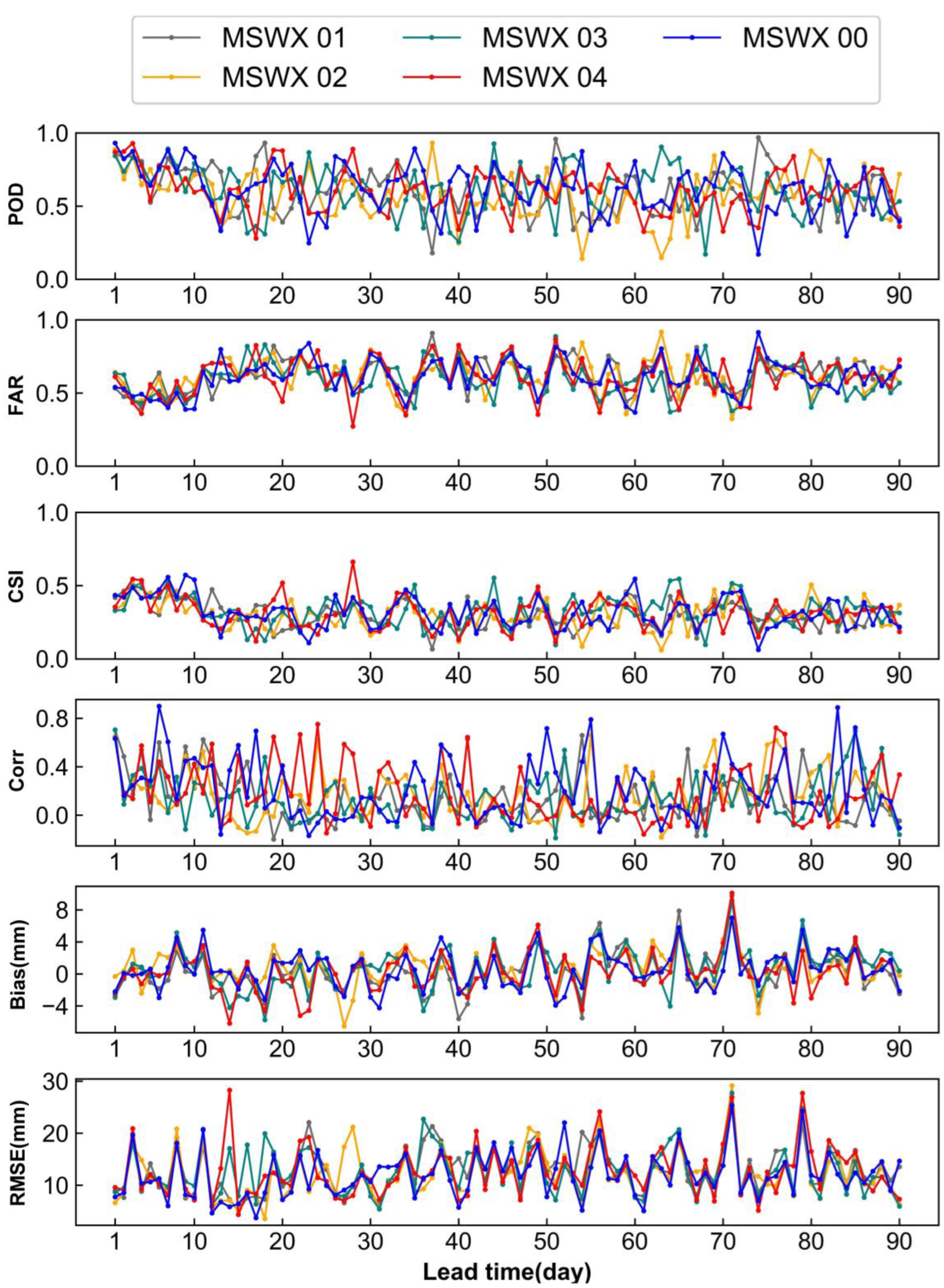
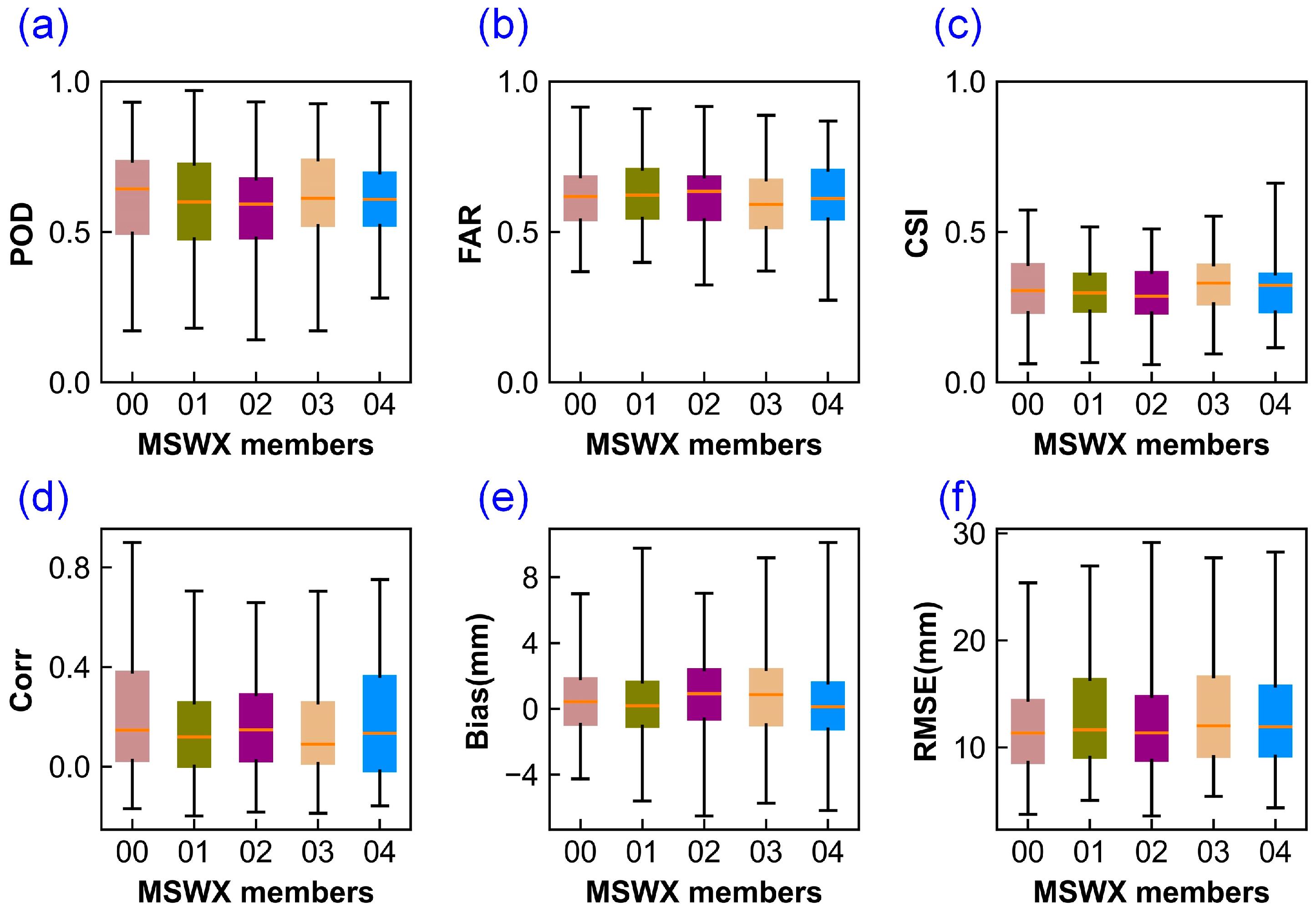
Figure 4 shows the precipitation detection efficiency (i.e., POD, FAR, CSI) and intensity forecast capability (i.e., Corr, BIAS, RMSE) of the MSWX members at various lead times. In terms of the POD metric, all MSWX ensemble members had significant performance fluctuations, ranging from 0.14 to 0.97. Similarly, the performance fluctuations of MSWX members on the FAR, CSI, Corr, BIAS, and RMSE metrics ranged from 0.27 to 0.92, 0.05 to 0.66, −0.20 to 0.90, −6.51 to 10.12 mm, and 3.57 to 29.15 mm, respectively. These fluctuations are also summarized in Figure 5. Overall, MSWX 00 exhibited relatively satisfactory performance with best performance values of 0.64, 0.14, and 11.33 mm in terms of medium POD, Corr, and RMSE, respectively. In addition, from the perspective of lead time, the error in MSWX members did not increase with the lead time. Therefore, MSWX had satisfactory value in supporting seasonal applications.
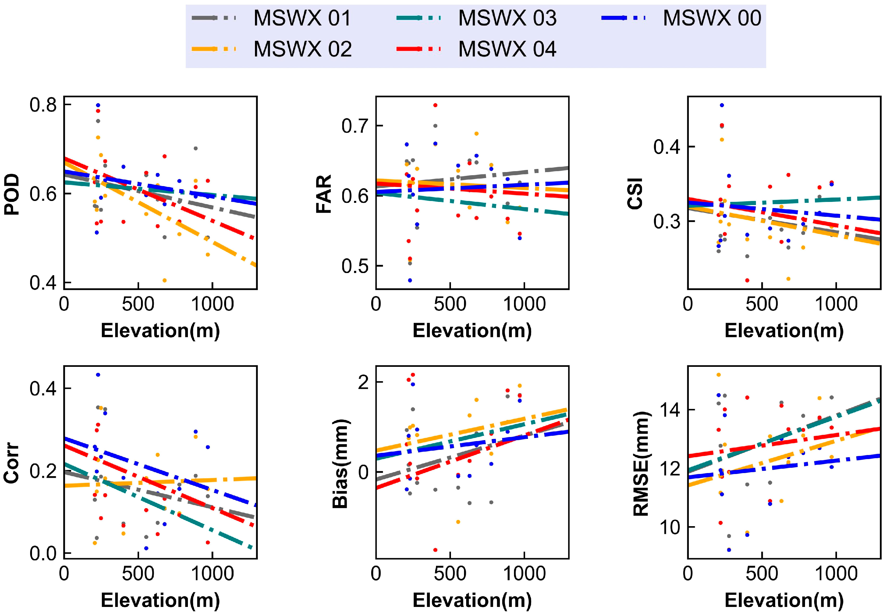
Figure 6 shows the performance characteristics of the MSWX members at different elevations. Generally, MSWX members tended to have worse accuracy at higher elevations. For example, MSWX 00 had CSI values of 0.46 and 0.35 at 229.254 m (BS station) and 968.824 m (DH station), respectively; MSWX 01 had CSI values of 0.43 and 0.28 at 229.254 m and 968.824 m, respectively. The decrease in performance along the elevation was also found for all other metrics. Overall, the MSWX 00 had the best performance with the smallest RMSE and relatively satisfying CSI and Corr.

4.2. Calibration and Validation of SWAT Hydrological Model

Before evaluating the hydrological performance of MSWX in runoff forecasting, the applicability of the SWAT hydrological model in the CR basin was investigated. In particular, a multi-site calibration approach was adopted to enhance the SWAT model to account for the spatial heterogeneity in hydrological behavior. Meanwhile, the gauge-based precipitation was used as input, and the SWAT was calibrated against runoff measurements. In addition, the NSE metric was used to qualitatively evaluate SWAT performance as this metric has a relatively clear benchmark (NSE = 0) [49]. The performance of SWAT is summarized in Table 4. Generally, the NSE values for SWAT during the calibration stage ranged from 0.61 to 0.80, while during the validation stage, the range was 0.68 to 0.79. The performance of the SWAT model in the XJ station was lower than that of the PT and BS stations, which may be attributed to the karst landscape distribution in the CR basin. Specifically, the control hydrological area of XJ Station is a karst landscape with complex underground culverts and karst pipelines, which increases the challenge of hydrological modeling. Overall, the SWAT had satisfactory performance (NSE ≥ 0.61), demonstrating its suitability for hydrologic modeling in CR Basin.
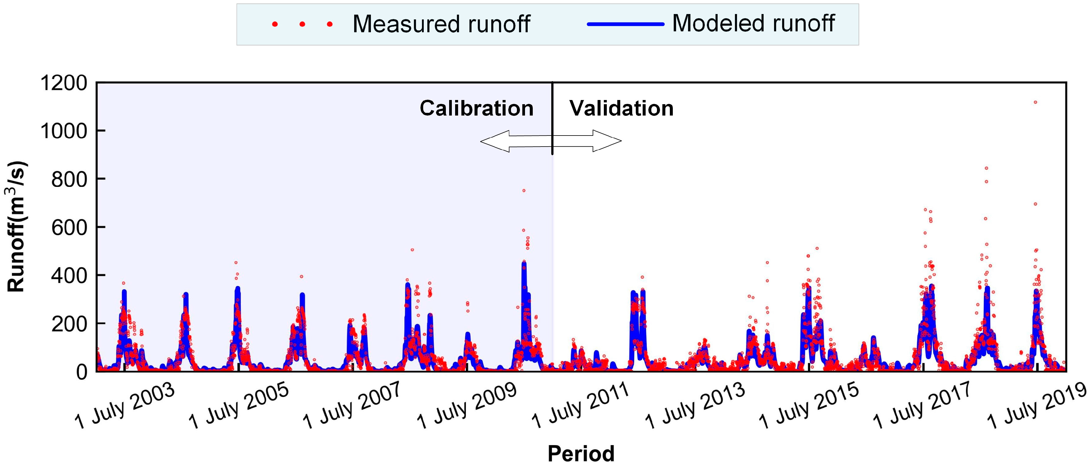
To further demonstrate the applicability of the SWAT model, the modeled runoff at the outlet of the CR basin was investigated. As shown in Figure 7, the modeled runoff was close to the observed runoff. Meanwhile, the modeled runoff reproduced the trend and seasonal cycle of measured runoff, albeit with a slight deviation in runoff peaks. For example, the modeled runoff exhibited flood peaks and peak occurrence times similar to measured runoff from 2011 to 2014. However, it is also important to note that the SWAT model also suffers from errors, especially in the simulation of high-runoff events from 2017 to 2019. Overall, the SWAT model based on multi-site calibration had good applicability in the CR basin and, hence, can be used for evaluating the hydrological performance of MSWX in runoff forecasting.

4.3. Hydrological Performance of MSWX in Runoff Forecasting

To evaluate the performance of MSWX in runoff forecasting, three precipitation input scenarios were considered in this study. Scenario 1, in which MSWX 00 forecasts were used as input precipitation. In Scenario 2, it was assumed that no new precipitation was generated during the forecast period, and this assumption is widely used in practical applications [50]. In Scenario 3, gauge-observed precipitation was used as the input. These runoff forecasting scenarios (methods) were referred to as MSWX-precipitation forecast, no-precipitation forecast, and station-precipitation simulation.
The forecast performance of different methods was evaluated four times per year (initialized at 0000 UTC on 1 January, 1 April, 1 July, and 1 October) from January 2014 through 2019. For the sake of convenience, these initialization times are numbered T1 to T24. For example, T1 and T24 stand for 1 January 2014 and 1 October 2019, respectively. In addition, the SWAT parameters were kept consistent with Section 4.2. These scenarios and methods are summarized in Table 5.
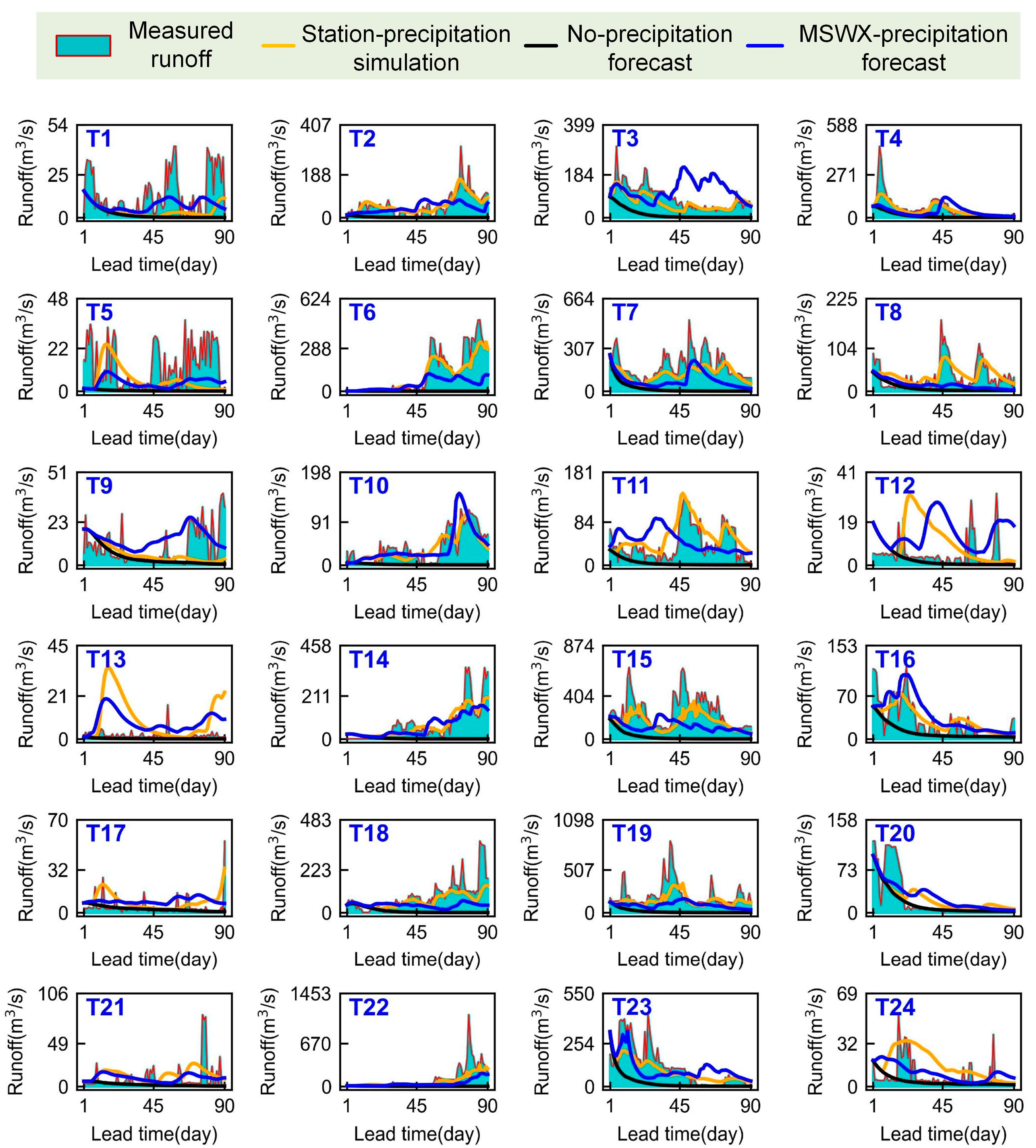
Figure 8 shows the forecast and measured runoff for the CR watershed outlet (BS station). Generally, the MSWX precipitation-based forecast could reflect the runoff trend to a certain extent compared with gauge observation. For example, at the T17, the MSWX forecast runoff exhibited a decreasing trend consistent with gauge observation. Similarly, at T6, T10, and T16, the MSWX forecast runoff exhibited an increasing trend consistent with gauge observation. Interestingly, MSWX performed better at moderate runoff events [runoff ~100 m3/s to 200 m3/s, e.g., Figure 8(T10)], but performed poorly at large runoff events [runoff > 250 m3/s; e.g., Figure 8(T4)]. In addition, compared with the No-precipitation forecast, there was less error in the MSWX forecast. The similarity between the No-precipitation forecast and observed runoff decreased with increasing lag time. For example, at the T17, the similarity between the No-precipitation forecast and the measured runoff decreased rapidly with time, while the MSWX-precipitation forecast captured the fluctuation of measured runoff. Similarly, at T7, T9, and T23, the MSWX-precipitation forecast exhibited better performance than the no-precipitation forecasts. Therefore, MSWX had some potential to be utilized in runoff forecasting with a long lag time.
The hydrological performance of MSWX in runoff forecasting was also quantitatively evaluated using multiple metrics. In particular, the specific runoff events are summarized in Table 6. As shown in Table 6, MSWX achieved satisfactory performance in nine runoff forecasts, which accounted for 22% of the total forecast events. Among the nine runoff events, the MSWX-based approach had Biases ranging from −10.62 to 65.37 m3/s with an average bias of 19.82 m3/s, suggesting that the approach tended to underestimate runoff. This underestimation was also verified in Figure 8. In addition to Bias, the Corr and RMSE of the MSWX-based approach ranged from 0.34 to 0.77 and from 24.46 to 164.28 m3/s, respectively.
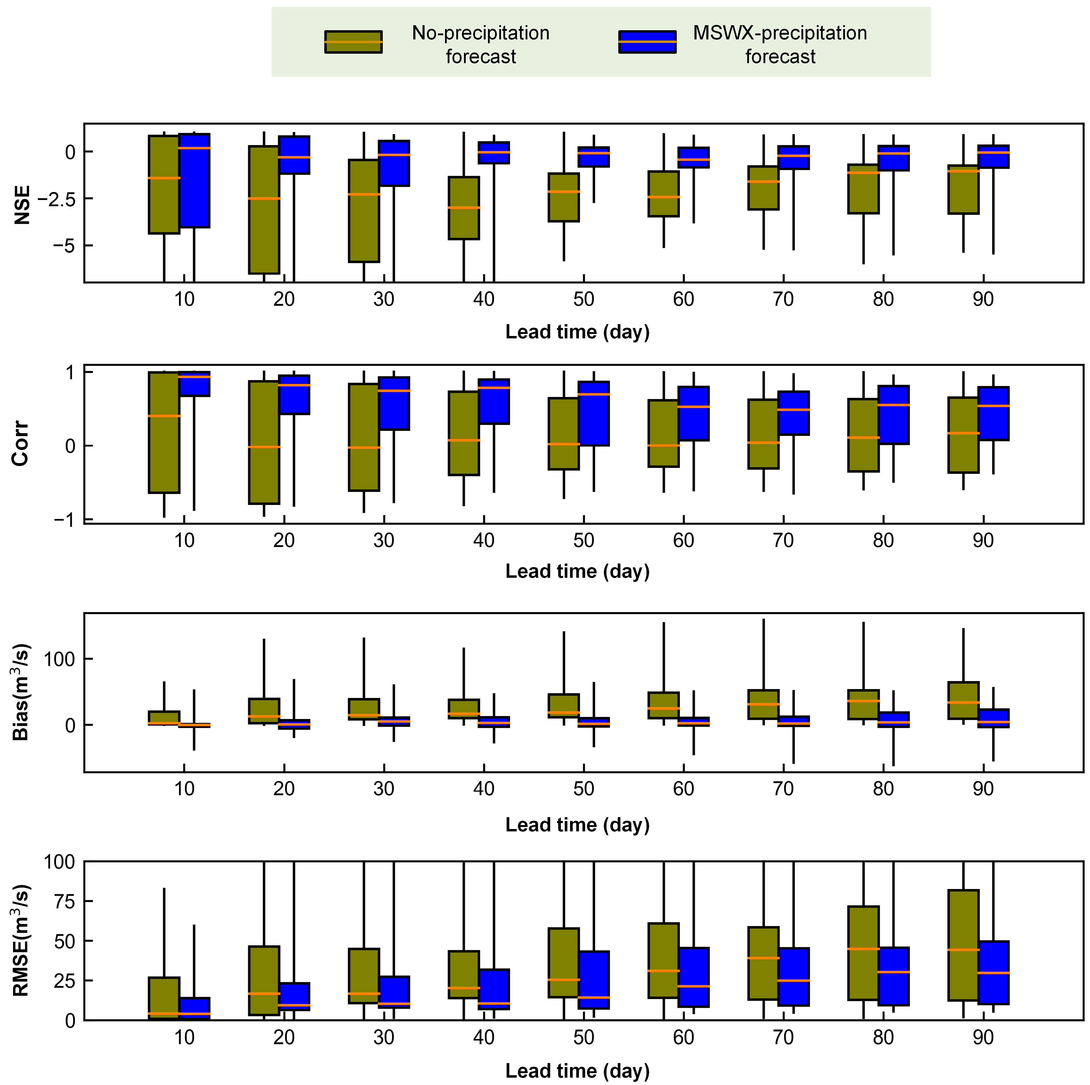
To analyze the skills of MSWX for runoff forecasting further, we compared its performance difference with that of the no-precipitation forecast. In particular, in the no-precipitation forecast scenario, station-measured precipitation at lag time = 0 was used as input of the SWAT model to forecast runoff at lag time = 0, 1, …, n, and no new precipitation was generated during the forecast period (i.e., t = 0, 1, …, n.). Meanwhile, station-precipitation simulation was used as a reference to evaluate the performance of the MSWX-precipitation forecast and No-precipitation forecast. As can be seen from Figure 8, the Bias of both the MSWX-precipitation forecast and the No-precipitation forecast increased with the increase of the lag times. However, the MSWX-precipitation forecast had a relatively small magnitude of increase. Similarly, the MSWX-precipitation forecast performed better than the No-precipitation forecast in terms of Bias and RMSE metrics. Overall, the MSWX-precipitation forecast had competitive performance in the short term (lead time ≤ 20 days) while showing significant advantages in the long-term runoff prediction (Figure 9).

5. Discussion

5.1. Unique Hydrometeorological Insights and Their Attributions

MSWX has provided new opportunities for reliable precipitation forecasts with fine horizontal resolution and long lead time. However, few studies have comprehensively evaluated the performance of MSWX in hill-karst basins. Therefore, we further discussed the accuracy characteristics of MSWX at different elevations and the skill of MSWX in supporting runoff forecasting. This study found that the MSWX tended to have lower accuracy at higher altitudes (Figure 6), which may be attributed to the regional precipitation system and the production strategy adopted in MSWX. Specifically, under the effect of mountainous terrain, the precipitation intensity of CR Basin tended to increase with increasing altitude (Table 1). Similar elevation-dependent patterns were also found in references [51,52]. However, the precipitation gauges near to CR basin used for error reduction in the MSWX product are located at low elevations (altitude ≤ 500 m) [20,53], thereby potentially resulting in better accuracy at low elevations. In addition, climatic processes at higher altitudes typically exhibited greater instability than at lower altitudes [54]. Specifically, the atmosphere is thinner at high altitudes, leading to a rapid spread of solar radiation and a pronounced heat dissipation effect [55]. This characteristic leads to large temperature variations at high altitudes, thereby leading to climate instability and increasing the technical difficulty of precipitation forecasting. Interestingly, the error of MSWX did not significantly increase with the increased lead time, which differs significantly from evaluations for similar precipitation products [56]. The possible reason for this is that a cumulative distribution correction is an effective approach to reducing the systematic bias that grows with lead times. Therefore, MSWX had satisfactory value in supporting meteorological applications. However, we found that the MSWX had limited skill in hydrological modeling. The probable cause of this phenomenon is the accumulation of errors in runoff forecasting. Fortunately, compared with precipitation-free runoff forecasting (Figure 8 and Figure 9), MSWX provided a significant advantage with a small increase in error with lag time. Therefore, MSWX is still useful in supporting runoff forecasting with non-negligible value.

5.2. Suggestions for MSWX Development and Applications

This study comprehensively evaluated the performance of MSWX for precipitation forecasting and hydrologic modeling, which can provide feedback to the development of MSWX and inform its applications. For example, MSWX tended to have lower accuracy at higher altitudes. However, the elevation-dependent phenomenon is highly non-linear (Figure 6). Therefore, machine learning techniques may be a suitable alternative for improving MSWX accuracy due to their strong non-linear modeling capabilities [57]. Some of the alternatives include support vector machines, regression trees, and artificial neural networks. In addition, this study found that the error in precipitation forecasting had not significantly increased with the increased lead time. Therefore, MSWX had satisfactory value in supporting long-term weather-related applications, including drought prevention and irrigation planning for agriculture. In addition, we found that MSWX provided a significant hydrological advantage compared with the no-precipitation forecast approach but increased in error with lag time (Figure 8). Therefore, the hydrological performance of MSWX may be improved by using post-processing methods, e.g., Bayesian model averaging [58] and Kalman filters [59]. Overall, attention needs to be paid to error accumulation in runoff forecasting applications.

5.3. Limitation and Future Research

Although this study provides some new hydrometeorological insights into the forecasting performance of MSWX, some limitations and further directions still need to be discussed. It should be specifically explained that owing to the lack of data, MSWX evaluation had to be conducted only in the CR basin. Errors in the SWAT model also introduced some uncertainty in the MSWX performance evaluation. Therefore, it is unrealistic to extrapolate the findings of this study to other regions with different topographies and climates; more similar evaluations should be conducted. In addition, accuracy and consistency tests were not conducted in this study due to limitations in the number and length of gauge data. Therefore, it is also important to evaluate MSWX performance over longer time scales to gain more reliable insights. In addition to precipitation, other MSWX forecast variables (e.g., pressure and humidity) are also worth evaluating in future studies.

6. Conclusions

The performance of multi-source weather was evaluated in terms of precipitation forecasting and runoff modeling in the Chengbi River Basin, a typical hill-karst region in southwest China. Meanwhile, multiple statistical metrics, the Soil and Water Assessment Tool (SWAT), and a multi-site calibration strategy were used in the evaluation process. We found that:
(1)
MSWX ensemble members tended to underestimate the number of no-precipitation events. Meanwhile, MSWX products tended to have worse accuracy at higher elevations. However, the error in MSWX members did not increase with the lead time.
(2)
The SWAT model based on multi-site calibration had good applicability in the CR Basin and performed well, with NSE values of 0.76 and 0.71 at the calibration and validation stages, respectively. Therefore, the model can be used for assessing the hydrological performance of MSWX in runoff forecasting.
(3)
MSWX provided a significant hydrological advantage compared with the traditional runoff forecast with precipitation-free assumption. Meanwhile, MSWX achieved satisfactory performance (NSE > 0) in 22% of runoff event predictions. However, the error increased with lag time.
MSWX has significant value in precipitation forecasting but limited skill in hydrologic modeling. Post-processing methods using elevation information should be considered in the future to improve MSWX performance. In addition, other MSWX variables are also worth evaluation.

Author Contributions

Conceptualization, C.M. and X.L.; Data curation, X.L. and X.C.; Formal analysis, X.W.; Funding acquisition, C.M., R.M., Y.H. and G.S.; Methodology, X.L. and X.C.; Project administration, C.M.; Resources, C.M., R.M., Y.H. and G.S.; Software, X.W.; Validation, X.L.; Visualization, X.L.; Writing—original draft, X.L. and X.C. All authors have read and agreed to the published version of the manuscript.

Funding

This research was funded by the National Natural Science Foundation of China (Grant Nos. 52269002 and 51969004) and the Guangxi Water Resource Technology Promotion Foundation (Grant No. SK2022-021).

Institutional Review Board Statement

Not applicable.

Informed Consent Statement

Not applicable.

Data Availability Statement

The data presented in this study are available on request from the corresponding author. The data are not publicly available due to policy constraints.

Conflicts of Interest

Author Yi Huang was employed by the company Guangxi Water & Power Design Institute Co., Ltd. Author Xinru Chen was employed by the company Shanghai Nuclear Engineering Research & Design Institute Co., Ltd. The remaining authors declare that the research was conducted in the absence of any commercial or financial relationships that could be construed as a potential conflict of interest.

References

  1. Kaune, A.; Chowdhury, F.; Werner, M.; Bennett, J. The benefit of using an ensemble of seasonal streamflow forecasts in water allocation decisions. Hydrol. Earth Syst. Sc. 2020, 24, 3851–3870. [Google Scholar] [CrossRef]
  2. Scaife, A.A.; Ferranti, L.; Alves, O.; Athanasiadis, P.; Baehr, J.; Dequé, M.; Dippe, T.; Dunstone, N.; Fereday, D.; Gudgel, R.G.; et al. Tropical rainfall predictions from multiple seasonal forecast systems. Int. J. Climatol. 2019, 39, 974–988. [Google Scholar] [CrossRef]
  3. Johnson, S.J.; Stockdale, T.N.; Ferranti, L.; Balmaseda, M.A.; Molteni, F.; Magnusson, L.; Tietsche, S.; Decremer, D.; Weisheimer, A.; Balsamo, G.; et al. SEAS5: The new ECMWF seasonal forecast system. Geosci. Model. Dev. 2019, 12, 1087–1117. [Google Scholar] [CrossRef]
  4. Camp, J.; Roberts, M.; MacLachlan, C.; Wallace, E.; Hermanson, L.; Brookshaw, A.; Arribas, A.; Scaife, A.A. Seasonal forecasting of tropical storms using the Met Office GloSea5 seasonal forecast system. Q. J. R. Meteor. Soc. 2015, 141, 2206–2219. [Google Scholar] [CrossRef]
  5. Wang, W.; Chen, M.; Kumar, A. An Assessment of the CFS Real-Time Seasonal Forecasts. Weather. Forecast. 2010, 25, 950–969. [Google Scholar] [CrossRef]
  6. Alves, O.; Wang, G.; Zhong, A.; Smith, N.; Tseitkin, F.; Warren, G.; Schiller, A.; Godfrey, S.; Meyers, G. POAMA: Bureau of Meteorology Operational Coupled Model Seasonal Forecast System; Bureau of Meteorology: Melbourne, Australia, 2003; pp. 49–56. [Google Scholar]
  7. Boas, T.; Bogena, H.R.; Ryu, D.; Vereecken, H.; Western, A.; Hendricks Franssen, H. Seasonal soil moisture and crop yield prediction with fifth-generation seasonal forecasting system (SEAS5) long-range meteorological forecasts in a land surface modelling approach. Hydrol. Earth Syst. Sci. 2023, 27, 3143–3167. [Google Scholar] [CrossRef]
  8. Arnal, L.; Cloke, H.L.; Stephens, E.; Wetterhall, F.; Prudhomme, C.; Neumann, J.; Krzeminski, B.; Pappenberger, F. Skilful seasonal forecasts of streamflow over Europe? Hydrol. Earth Syst. Sci. 2018, 22, 2057–2072. [Google Scholar] [CrossRef]
  9. Neta, A.; Levi, Y.; Morin, E.; Morin, S. Seasonal forecasting of pest population dynamics based on downscaled SEAS5 forecasts. Ecol. Model. 2023, 480, 110326. [Google Scholar] [CrossRef]
  10. Bi, K.; Xie, L.; Zhang, H.; Chen, X.; Gu, X.; Tian, Q. Accurate medium-range global weather forecasting with 3D neural networks. Nature 2023, 619, 533–538. [Google Scholar] [CrossRef]
  11. Duan, Q.; Pappenberger, F.; Wood, A.; Cloke, H.L.; Schaake, J.C. Handbook of Hydrometeorological Ensemble Forecasting; Springer: Berlin/Heidelberg, Germany, 2019; Volume 10. [Google Scholar]
  12. Beck, H.E.; Pan, M.; Roy, T.; Weedon, G.P.; Pappenberger, F.; van Dijk, A.I.J.M.; Huffman, G.J.; Adler, R.F.; Wood, E.F. Daily evaluation of 26 precipitation datasets using Stage-IV gauge-radar data for the CONUS. Hydrol. Earth Syst. Sci. 2019, 23, 207–224. [Google Scholar] [CrossRef]
  13. Mo, C.; Lei, X.; Mo, X.; Ruan, R.; Tang, G.; Li, L.; Sun, G.; Jiang, C. Comprehensive evaluation and comparison of ten precipitation products in terms of accuracy and stability over a typical mountain basin, Southwest China. Atmos. Res. 2024, 297, 107116. [Google Scholar] [CrossRef]
  14. Wang, Q.J.; Shao, Y.; Song, Y.; Schepen, A.; Robertson, D.E.; Ryu, D.; Pappenberger, F. An evaluation of ECMWF SEAS5 seasonal climate forecasts for Australia using a new forecast calibration algorithm. Environ. Modell. Softw. 2019, 122, 104550. [Google Scholar] [CrossRef]
  15. Hudson, D.; Alves, O.; Hendon, H.H.; Marshall, A.G. Bridging the gap between weather and seasonal forecasting: Intraseasonal forecasting for Australia. Q. J. R. Meteorol. Soc. 2011, 137, 673–689. [Google Scholar] [CrossRef]
  16. Wu, Z.; Yin, H.; He, H.; Li, Y. Dynamic-LSTM hybrid models to improve seasonal drought predictions over China. J. Hydrol. 2022, 615, 128706. [Google Scholar] [CrossRef]
  17. White, C.J.; Carlsen, H.; Robertson, A.W.; Klein, R.J.T.; Lazo, J.K.; Kumar, A.; Vitart, F.; Coughlan De Perez, E.; Ray, A.J.; Murray, V.; et al. Potential applications of subseasonal-to-seasonal (S2S) predictions. Meteorol. Appl. 2017, 24, 315–325. [Google Scholar] [CrossRef]
  18. Chevuturi, A.; Turner, A.G.; Johnson, S.; Weisheimer, A.; Shonk, J.K.P.; Stockdale, T.N.; Senan, R. Forecast skill of the Indian monsoon and its onset in the ECMWF seasonal forecasting system 5 (SEAS5). Clim. Dynam 2021, 56, 2941–2957. [Google Scholar] [CrossRef]
  19. Ferreira, G.W.S.; Reboita, M.S.; Drumond, A. Evaluation of ECMWF-SEAS5 Seasonal Temperature and Precipitation Predictions over South America. Climate 2022, 10, 128. [Google Scholar] [CrossRef]
  20. Beck, H.E.; van Dijk, A.I.J.M.; Larraondo, P.R.; McVicar, T.R.; Pan, M.; Dutra, E.; Miralles, D.G. MSWX Global 3-Hourly 0.1° Bias-Corrected Meteorological Data Including Near-Real-Time Updates and Forecast Ensembles. Bull. Am. Meteorol. Soc. 2022, 103, 710–732. [Google Scholar] [CrossRef]
  21. Hafizi, H.; Sorman, A.A. Integrating Meteorological Forcing from Ground Observations and MSWX Dataset for Streamflow Prediction under Multiple Parameterization Scenarios. Water 2022, 14, 2721. [Google Scholar] [CrossRef]
  22. Peel, M.C.; McMahon, T.A. Historical development of rainfall-runoff modeling. Wiley Interdiscip. Rev. Water 2020, 7, e1471. [Google Scholar] [CrossRef]
  23. Yao, C.; Ye, J.; He, Z.; Bastola, S.; Zhang, K.; Li, Z. Evaluation of flood prediction capability of the distributed Grid-Xinanjiang model driven by weather research and forecasting precipitation. J. Flood Risk Manag. 2019, 12, e12544. [Google Scholar] [CrossRef]
  24. Arnold, J.G.; Moriasi, D.N.; Gassman, P.W.; Abbaspour, K.C.; White, M.J.; Srinivasan, R.; Santhi, C.; Harmel, R.D.; Van Griensven, A.; Van Liew, M.W. SWAT: Model use, calibration, and validation. Trans. ASABE 2012, 55, 1491–1508. [Google Scholar] [CrossRef]
  25. Arnold, J.G.; Srinivasan, R.; Muttiah, R.S.; Williams, J.R. Large area hydrologic modeling and assessment part I: Model development 1. Jawra J. Am. Water Resour. Assoc. 1998, 34, 73–89. [Google Scholar] [CrossRef]
  26. Hamman, J.J.; Nijssen, B.; Bohn, T.J.; Gergel, D.R.; Mao, Y. The Variable Infiltration Capacity model version 5 (VIC-5): Infrastructure improvements for new applications and reproducibility. Geosci. Model. Dev. 2018, 11, 3481–3496. [Google Scholar] [CrossRef]
  27. Beven, K.J.; Kirkby, M.J.; Freer, J.E.; Lamb, R. A history of TOPMODEL. Hydrol. Earth Syst. Sci. 2021, 25, 527–549. [Google Scholar] [CrossRef]
  28. Krysanova, V.; White, M. Advances in water resources assessment with SWAT—An overview. Hydrol. Sci. J. 2015, 60, 1–13. [Google Scholar] [CrossRef]
  29. Chen, J.; Cao, X.; Peng, S.; Ren, H. Analysis and Applications of GlobeLand30: A Review. Isprs Int. J. Geo-Inf. 2017, 6, 230. [Google Scholar] [CrossRef]
  30. Nachtergaele, F.; van Velthuizen, H.; Verelst, L.; Wiberg, D.; Henry, M.; Chiozza, F.; Yigini, Y.; Aksoy, E.; Batjes, N.; Boateng, E. Harmonized World Soil Database version 2.0; Food and Agriculture Organization of the United Nations: Rome, Italy, 2023. [Google Scholar]
  31. Mo, C.; Lai, S.; Yang, Q.; Huang, K.; Lei, X.; Yang, L.; Yan, Z.; Jiang, C. A comprehensive assessment of runoff dynamics in response to climate change and human activities in a typical karst watershed, southwest China. J. Environ. Manag. 2023, 332, 117380. [Google Scholar] [CrossRef]
  32. Stevanović, Z. Global distribution and use of water from karst aquifers. Geol. Soc. Lond. Spec. Publ. 2018, 466, 217–236. [Google Scholar] [CrossRef]
  33. Mo, C.; Tang, P.; Huang, K.; Lei, X.; Lai, S.; Deng, J.; Bao, M.; Sun, G.; Xing, Z. Evolution of Drought Trends under Climate Change Scenarios in Karst Basin. Water 2023, 15, 1934. [Google Scholar] [CrossRef]
  34. Sodoudi, S.; Noorian, A.; Geb, M.; Reimer, E. Daily precipitation forecast of ECMWF verified over Iran. Theor. Appl. Climatol. 2010, 99, 39–51. [Google Scholar] [CrossRef]
  35. WMO. Guide to Hydrological Practice. Hydrology—From Measurement to Hydrological Information; WMO: Geneva, Switzerland, 2008; Volume 1, p. 48. Available online: https://library.wmo.int/doc_num.php?explnum_id=10473 (accessed on 8 February 2023).
  36. Mo, C.; Ruan, Y.; Xiao, X.; Lan, H.; Jin, J. Impact of climate change and human activities on the baseflow in a typical karst basin, Southwest China. Ecol. Indic. 2021, 126, 107628. [Google Scholar] [CrossRef]
  37. Khan, M.K.U.; Iqbal, M.F.; Mahmood, I.; Shahzad, M.I.; Zafar, Q.; Khalid, B. Evaluation of precipitation products over different climatic zones of Pakistan. Theor. Appl. Climatol. 2023, 151, 1301–1321. [Google Scholar] [CrossRef]
  38. Huang, Z.; Zhao, T. Predictive performance of ensemble hydroclimatic forecasts: Verification metrics, diagnostic plots and forecast attributes. Wires Water 2022, 9, e1580. [Google Scholar] [CrossRef]
  39. WMO. Precipitation Estimation and Forecasting; WMO: Geneva, Switzerland, 2008; p. 6. Available online: https://library.wmo.int/doc_num.php?explnum_id=1708 (accessed on 10 February 2023).
  40. MWR; PRC. Specification for Precipitation Observations: SL 21-2015. Available online: https://std.samr.gov.cn/hb/search/stdHBDetailed?id=8B1827F15073BB19E05397BE0A0AB44A (accessed on 8 January 2023).
  41. Santhi, C.; Arnold, J.G.; Williams, J.R.; Dugas, W.A.; Srinivasan, R.; Hauck, L.M. Validation of the swat model on a large rwer basin with point and nonpoint sources. Jawra J. Am. Water Resour. Assoc. 2001, 37, 1169–1188. [Google Scholar] [CrossRef]
  42. Abbaspour, K.C.; Vaghefi, S.A.; Yang, H.; Srinivasan, R. Global soil, landuse, evapotranspiration, historical and future weather databases for SWAT Applications. Sci. Data 2019, 6, 263. [Google Scholar] [CrossRef]
  43. Aloui, S.; Mazzoni, A.; Elomri, A.; Aouissi, J.; Boufekane, A.; Zghibi, A. A review of Soil and Water Assessment Tool (SWAT) studies of Mediterranean catchments: Applications, feasibility, and future directions. J. Environ. Manag. 2023, 326, 116799. [Google Scholar] [CrossRef]
  44. López-Ballesteros, A.; Nielsen, A.; Castellanos-Osorio, G.; Trolle, D.; Senent-Aparicio, J. DSOLMap, a novel high-resolution global digital soil property map for the SWAT+ model: Development and hydrological evaluation. Catena 2023, 231, 107339. [Google Scholar] [CrossRef]
  45. Mo, C.; Zhang, M.; Ruan, Y.; Qin, J.; Wang, Y.; Sun, G.; Xing, Z. Accuracy Analysis of IMERG Satellite Rainfall Data and Its Application in Long-term Runoff Simulation. Water 2020, 12, 2177. [Google Scholar] [CrossRef]
  46. Kim, N.W.; Lee, J.W.; Lee, J.; Lee, J.E. SWAT application to estimate design runoff curve number for South Korean conditions. Hydrol. Process 2010, 24, 2156–2170. [Google Scholar] [CrossRef]
  47. Chien, H.; Yeh, P.J.F.; Knouft, J.H. Modeling the potential impacts of climate change on streamflow in agricultural watersheds of the Midwestern United States. J. Hydrol. 2013, 491, 73–88. [Google Scholar] [CrossRef]
  48. Nash, J.E.; Sutcliffe, J.V. River flow forecasting through conceptual models part I—A discussion of principles. J. Hydrol. 1970, 10, 282–290. [Google Scholar] [CrossRef]
  49. Knoben, W.J.M.; Freer, J.E.; Woods, R.A. Technical note: Inherent benchmark or not? Comparing Nash-Sutcliffe and Kling-Gupta efficiency scores. Hydrol. Earth Syst. Sci. 2019, 23, 4323–4331. [Google Scholar] [CrossRef]
  50. Dou, Y.; Ye, L.; Gupta, H.V.; Zhang, H.; Behrangi, A.; Zhou, H. Improved Flood Forecasting in Basins with No Precipitation Stations: Constrained Runoff Correction Using Multiple Satellite Precipitation Products. Water Resour. Res. 2021, 57, e2021WR029682. [Google Scholar] [CrossRef]
  51. Singh, P.; Kumar, N. Effect of orography on precipitation in the western Himalayan region. J. Hydrol. 1997, 199, 183–206. [Google Scholar] [CrossRef]
  52. Zavala, V.; Carretier, S.; Bonnet, S. Influence of orographic precipitation on the topographic and erosional evolution of mountain ranges. Basin Res. 2020, 32, 1574–1599. [Google Scholar] [CrossRef]
  53. Karger, D.N.; Conrad, O.; Böhner, J.; Kawohl, T.; Kreft, H.; Soria-Auza, R.W.; Zimmermann, N.E.; Linder, H.P.; Kessler, M. Climatologies at high resolution for the earth’s land surface areas. Sci. Data 2017, 4, 170122. [Google Scholar] [CrossRef]
  54. Gebregiorgis, A.S.; Hossain, F. Understanding the Dependence of Satellite Rainfall Uncertainty on Topography and Climate for Hydrologic Model Simulation. IEEE Trans. Geosci. Remote 2013, 51, 704–718. [Google Scholar] [CrossRef]
  55. Pepin, N.; Bradley, R.S.; Diaz, H.F.; Baraer, M.; Caceres, E.B.; Fowler, N.F.H. Elevation-dependent warming in mountain regions of the world. Nat. Clim. Change 2015, 5, 424–430. [Google Scholar] [CrossRef]
  56. Donegan, S.; Murphy, C.; Harrigan, S.; Broderick, C.; Foran Quinn, D.; Golian, S.; Knight, J.; Matthews, T.; Prudhomme, C.; Scaife, A.A.; et al. Conditioning ensemble streamflow prediction with the North Atlantic Oscillation improves skill at longer lead times. Hydrol. Earth Syst. Sci. 2021, 25, 4159–4183. [Google Scholar] [CrossRef]
  57. Frnda, J.; Durica, M.; Rozhon, J.; Vojtekova, M.; Nedoma, J.; Martinek, R. ECMWF short-term prediction accuracy improvement by deep learning. Sci. Rep. 2022, 12, 7898. [Google Scholar] [CrossRef] [PubMed]
  58. Xu, J.; Anctil, F.; Boucher, M. Hydrological post-processing of streamflow forecasts issued from multimodel ensemble prediction systems. J. Hydrol. 2019, 578, 124002. [Google Scholar] [CrossRef]
  59. Khaki, M.; Ait-El-Fquih, B.; Hoteit, I. Calibrating land hydrological models and enhancing their forecasting skills using an ensemble Kalman filter with one-step-ahead smoothing. J. Hydrol. 2020, 584, 124708. [Google Scholar] [CrossRef]
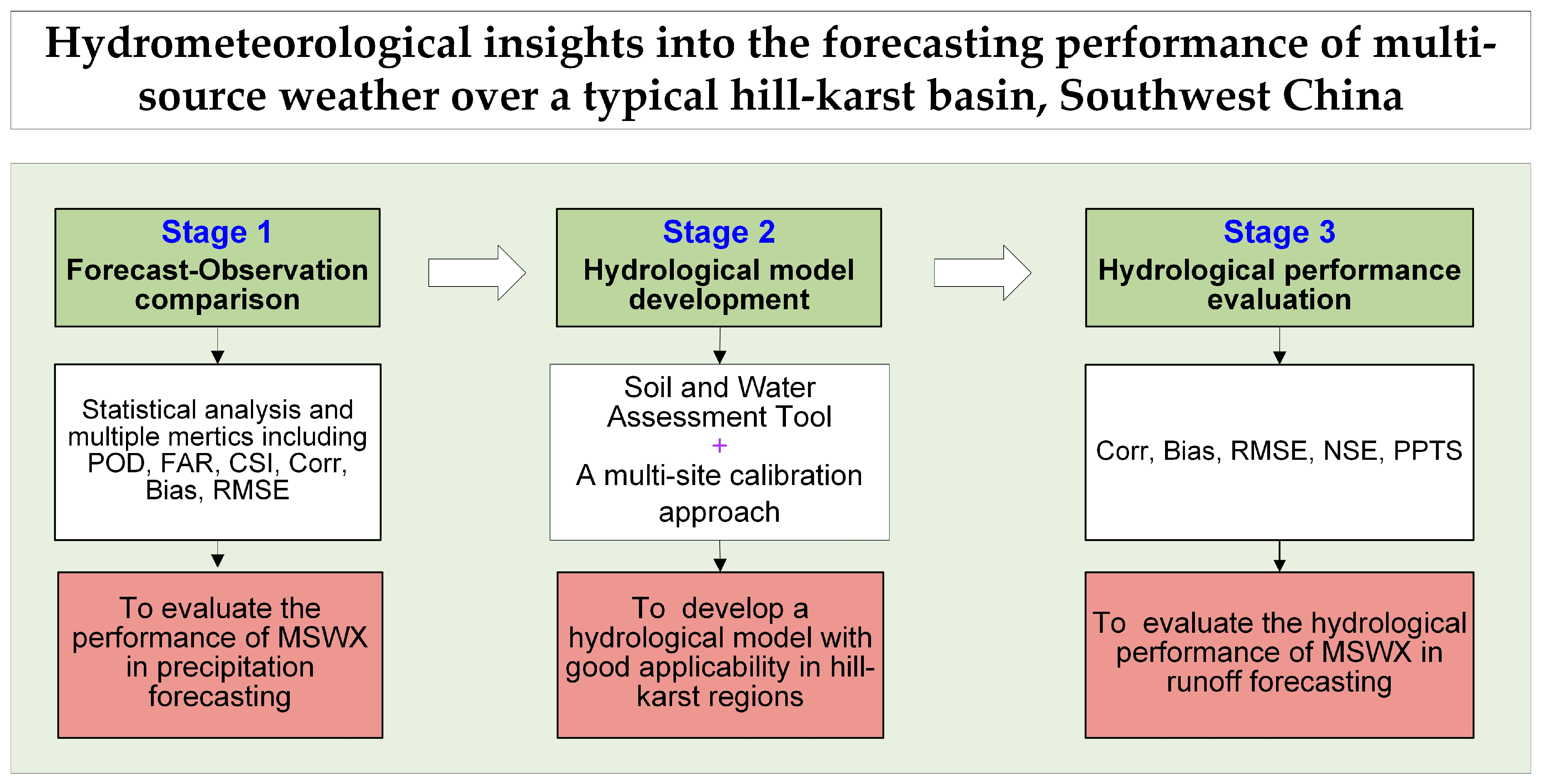
Figure 1. The structure chart of the study.
Atmosphere 15 00236 g001
Figure 2. Approximate profiles of the CR basin: (a) location of CR basin in China, (b) hydrometeorological station distribution and altitude topographic map under MSWX grids, and (c) hydrometeorological station distribution under the hypsometric curve of the CR Basin. The “relative area” refers to the percentage ratio of the area of a specific region, which is at an altitude lower than a certain value, to the total area of the entire watershed.
Atmosphere 15 00236 g002
Figure 3. Statistical analysis of precipitation data from different sources: (a) percentage of precipitation events in each precipitation dataset, and (b) cumulative probability distribution of observed and forecast precipitation under different intensities (exclusion intensity < 1 mm/day).
Atmosphere 15 00236 g003
Figure 4. Performance characteristics of MSWX members at different lead times.
Atmosphere 15 00236 g004
Figure 5. Statistical analysis of the accuracy fluctuation of different MSWX members. The upper and lower lines of the box and the middle line represent the 25th and 75th percentile and median, respectively, while “whiskers” indicate extreme values. The (af) represent POD, FAR, CSI, Corr, Bias, and RMSE metrics, respectively.
Atmosphere 15 00236 g005
Figure 6. Scatterplot and the fitted line of accuracy metrics versus elevation for various MSWX memberships.
Atmosphere 15 00236 g006
Figure 7. Performance of the multi-site calibration-based SWAT for the calibration stage and validation stage.
Atmosphere 15 00236 g007
Figure 8. Performance of different precipitation data in runoff prediction. T1–T24 represents different initialization times from 2014 to 2019 at 3-month intervals. For example, T1 and T24 stand for 1 January 2014 and 1 October 2019, respectively.
Atmosphere 15 00236 g008
Figure 9. Performance of different precipitation data in runoff prediction benchmarked against gauge-precipitation simulations. The upper and lower lines of the box and the middle (orange) line represent the 25th and 75th percentile and median, respectively, while “whiskers” indicate extreme values. Some of the extremes are not fully shown, as the distance from the percentile is too large.
Atmosphere 15 00236 g009
Table 1. Hydrometeorological stations used for performance evaluation.
StationMeasured ElementsLongitude (°)Latitude (°)Altitude (m)Average Annual Precipitation (mm)
BS (Bashou)Daily precipitation and runoff106.6423.95229.251072.89
PT (Pingtang)Daily precipitation and runoff106.6524.09276.811256.92
XJ (Xiajia)Daily precipitation and runoff106.6524.29554.131531.93
HK (Haokun)Daily precipitation106.6624.19399.961442.04
LY (Linyun)Daily precipitation106.5724.35630.471687.12
CL (Chaoli)Daily precipitation106.5024.24777.371466.88
XT (Xiatang)Daily precipitation106.5524.04207.231101.36
DH (Donghe)Daily precipitation106.7224.36968.821588.76
JF (Jiefu)Daily precipitation106.8024.32677.771668.25
NT (Nongtang)Daily precipitation106.7624.21886.981502.75
LH (Linhe)Daily precipitation106.7024.06248.28961.25
BL (Bailian)Daily precipitation106.7523.96220.441086.94
Table 2. Summary of MSWX members evaluated in this study.
MSWX MemberInput DataBias Correction MethodSpatial ResolutionTemporal ResolutionReference Climatologies
MSWX 00SEAS5 00A CDF-matching approach0.1°1dMSWX Past subproduct
MSWX 01SEAS5 01
MSWX 02SEAS5 02
MSWX 03SEAS5 03
MSWX 04SEAS5 04
Table 3. Quantitative metrics used in this study for MSWX performance evaluation.
MetricFormulaRangeUnbiased ValueFormula No.
POD P O D = H H + M [0, 1]1(1)
FAR F A R = F H + F [0, 1]0(2)
CSI P O D = H H + M + F [0, 1]1(3)
Corr C o r r = t = 1 n P MSWX ( t ) P MSWX ¯ P station   ( t ) P station   ¯ t = 1 n P MSWX ( t ) P MSWX ¯ 2 i = 1 n P station   ( t ) P station   ¯ 2 [−1, 1]1(4)
Bias B i a s = t = 1 n P station   ( t ) P MSWX ( t ) n (−∞, +∞)0(5)
RMSE R M S E = 1 N t = 1 N P station   ( t ) P MSWX ( t ) 2 [0, +∞)1(6)
Note that: H is the number of precipitation events detected by both the MSWX product and station device; M is the number of unpredicted but observed precipitation events; F denotes the number of predicted but unobserved precipitation events; P s t a t i o n and P M S W X denote the observed and predicted precipitation intensities, respectively; P station ¯ and P MSWX ¯ represent the mean value of observations and forecasts, respectively; N indicates the evaluation sample size. The threshold for distinguishing between precipitation and non-precipitation events was set as 1 mm/d according to the local standard [40].
Table 4. Performance of SWAT based on multi-site calibration during calibration and validation stages.
StationStageNSE
XJCalibration (2003–2010)0.61
Validation (2011–2017)0.68
PTCalibration (2003–2010)0.80
Validation (2011–2019)0.79
BSCalibration (2003–2010)0.76
Validation (2011–2019)0.71
Note: Only these stations (i.e., XJ, PT, and BS) measure runoff information and, therefore, were selected for hydrologic modeling.
Table 5. Summary of different runoff prediction scenarios and methods.
Scenario NumberMethod NamePrecipitation InputInitialization TimeLead Time (d)
1MSWX-precipitation forecastMSWX 001 January, 1 April, 1 July, and 1 October from January 2014 through 2019, which are numbered chronologically as T1 through T24.1–90
2No-precipitation forecastNone
3Station-precipitation simulationGauge observations
Table 6. Performance of MSWX product in runoff forecasting against gauge runoff measurements.
Runoff EventInitialization TimeNSECorrBias (m3/s)RMSE (m3/s)PPTS (90)(%)
T11 January 2014−0.040.445.6513.0875.60
T21 March 20140.070.3411.4650.6576.10
T31 July 2014−1.81−0.39−34.4586.2752.95
T41 October 20140.080.4020.9270.6882.86
T51 January 2015−0.500.188.3914.0885.83
T61 March 20150.050.6770.26141.2190.69
T71 July 2015−0.830.5797.92123.6165.21
T81 October 2015−0.430.0119.8140.3393.33
T91 January 2016−0.230.28−4.9410.8175.02
T101 March 20160.340.68−0.2729.0425.19
T111 July 2016−0.84−0.36−6.3644.2368.70
T121 October 2016−4.14−0.15−9.2613.1340.38
T131 January 2017−18.970.06−6.418.0368.01
T141 March 20170.500.7411.5063.6864.56
T151 July 2017−0.92−0.02132.60204.6783.85
T161 October 20170.330.72−10.6224.6411.56
T171 January 2018−0.61−0.03−4.908.6487.03
T181 March 2018−0.37−0.0546.0892.3589.32
T191 July 2018−0.570.20112.68180.9987.17
T201 October 20180.550.77−3.7225.3825.03
T211 January 2019−0.060.02−1.3615.0086.80
T221 March 20190.180.6865.37164.2891.93
T231 July 20190.280.5413.5096.8288.37
T241 October 2019−0.140.24−2.7110.4966.80
Disclaimer/Publisher’s Note: The statements, opinions and data contained in all publications are solely those of the individual author(s) and contributor(s) and not of MDPI and/or the editor(s). MDPI and/or the editor(s) disclaim responsibility for any injury to people or property resulting from any ideas, methods, instructions or products referred to in the content.