Abstract
In order to mitigate the impact of particulate pollutants in Nanjing Sample Industrial Park, it is imperative to simulate the wind field and pollutant dispersion inside the park. Therefore, a CFD-DPM study was employed to simulate the wind field and pollutant dispersion with an accurate landform model. A large eddy simulation was utilized for calculating wind flow distribution inside the park, which is more suitable than Reynolds-Averaged Navier–Stokes Equations (RANS). The physical model of the plant canopy was incorporated to assess its influence on the wind field and particulate pollutants through drag, buoyancy, and deposition effects. Using this method, the distributions of the wind field, and contaminant and the sensitivity tests were obtained by means of calculating a number of research cases under different meteorological conditions. In the numerical results, the wind field was obstructed by the plant canopy, resulting in near-ground uniformity under unstable weather conditions. The distribution of particulate pollutants was influenced not only by the drag and buoyancy effects but also by deposition, which caused an accumulation of particulate pollutants on the windward side of the canopy under unstable weather conditions. The sensitivity tests were performed by comparing the concentrations of particulate pollutants under various conditional settings. The canopy regions can remove the particulate pollutant by 50% under stable weather conditions. The deposition effect is enhanced by larger particle density and diameter and is also influenced by leaf area density.
1. Introduction
Atmospheric pollution poses a significant threat to human health, particularly in industrial parks where the emissions of particulate pollutants from factories can cause severe damage to the respiratory system. To mitigate this risk and protect individuals within the parks, it is crucial to monitor the distribution of air pollution. Therefore, studying the dispersion characteristics of air pollutants, especially particulate matter, becomes essential. When the contamination leaks in the industrial park, the concentration distribution around the pollutant source can be obtained by predicting the dispersion direction and speed of pollutant [1,2,3]. However, further research is needed to investigate the details and mechanisms of pollutant dispersion in industrial parks [4]. As a result, a real case study with a numerical calculation model was conducted to investigate the dispersion of particulate pollutants in Nanjing Sample Industrial Park.
Compared to wind tunnel experiments and field measurements, Computational Fluid Dynamics (CFD) is increasingly crucial for investigating flow behaviors and contaminant dispersion in urban environments [5]. The utilization of CFD eliminates the need for manufacturing complex landform models in wind tunnel experiments and reduces the resource expenditure required for establishing measurement points in field measurements. CFD has been extensively employed in contamination control studies due to its convenience, lower resource costs, and ability to provide detailed distributions of wind fields and pollutant concentrations through global simulations [6]. Table 1 presents a summary of research on computational simulation of flow fields as well as contaminant distribution and dispersion at an urban scale. Further details will be discussed below.
Atmospheric motion is a typical turbulent flow that contains complex wind flow and pollutant dispersion. Currently, Large Eddy Simulation (LES) is commonly employed instead of Reynolds-Averaged Navier–Stokes equations (RANS) to simulate atmospheric motion due to its ability to capture intricate features of turbulent flows [7,8,9]. Furthermore, it is difficult for RANS to simulate the impact of solar radiation on the flows [10]. Therefore, LES is adopted in this study.
CFD studies on atmospheric motion have gained popularity in recent years. Liu et al. [11] investigated the wind field and pollutant dispersion in downtown Macao using LES and a combined model that considered buildings as roughness elements. Hanna et al. [12] compared simulation results with experimental data to examine the behavior of mean flow and turbulence within simple obstacle arrays, revealing that the street canyon effect was more pronounced at higher flow speeds inside square arrays than staggered arrays. Wang and McNamara [13] assessed the applicability of RANS methods in simulating pollutant dispersion within idealized building arrays, highlighting significant differences between CFD and wind tunnel tests due to inadequate modeling of local flow patterns using RANS models. Previous studies primarily focused on the flow behaviors and pollutant dispersion in mesoscale atmospheric motion, lacking detailed information about building array interiors. Idealized street canyon models served as preliminary approaches for understanding turbulent flows around buildings, while further research is needed to investigate real case scenarios at micro meteorological scales.
Furthermore, Steffens et al. [14] investigated the transport of pollutants around roadside vegetation barriers, while Xie et al. [15] examined the impact of solar radiation on wind flow, highlighting the significance of incorporating plant canopy as a crucial parameter in atmospheric motion simulations. In a study conducted by Punyisa Chaisri and Pimporn Ponpesh [16], airflow fields and PM2.5 dispersion in Bangkok were analyzed using ANSYS 19.2 with the RANS-DPM method; however, this research did not consider the plant canopy model or solar radiation effect. Meng et al. [17] employed the RNG-DPM model in the FLUENT 18.0 software package to simulate PM2.5 distributions without considering canopy effects due to idealized building arrays. Consequently, there remains a dearth of real case studies investigating particulate pollutant dispersion with the inclusion of canopy models.
The present study conducts a real case investigation on wind flow and dispersion of particulate pollutants within Nanjing Sample Industrial Park. A precise terrain model is established to facilitate micro meteorological scale simulation, while employing the LES-DPM method and plant canopy model for accurate calculation of wind flow and dispersion of particulate pollutants.

Table 1.
Literature on computational simulation of flow field and contaminant distribution and dispersion at the urban scale.
Table 1.
Literature on computational simulation of flow field and contaminant distribution and dispersion at the urban scale.
| Reference | Research Object | Pollutant | Computational Model | Result |
|---|---|---|---|---|
| Liu et al., 2011 [11] | Wind field and pollutant dispersion in downtown Macao. | Gas (traffic exhaust) | Large Eddy Simulation (LES), a roughness element model of buildings. | The proposed model was an appropriate method for numerical prediction of urban atmospheric environment. |
| Wang and McNamara, 2006 [13] | Pollutant dispersion inside idealized building arrays. | Gas (Ethane) | Reynolds-Averaged Navier–Stokes equations (RANS). | The inadequate modeling of local flow patterns led to a deviation value compared with wind tunnel tests. |
| Steffens et al., 2013 [14] | Pollutant transport around roadside vegetation barriers. | Particulate matter | Continuous phase: RANS. Dispersed phase: Discrete Phase Model (DPM). | The model would be improved by using LES and the deposition effect of particles was significant in the simulation of pollutant dispersion. |
| Xie et al., 2005 [15] | Pollutant distribution inside idealized street canyon under the effect of solar radiation. | Gas (CO) | RANS and Boussinesq’s hypothesis. | The flow structure and contaminant distribution could be completely different under solar heating. |
| Punyisa Chaisri and Pimporn Ponpesh, 2022 [16] | Airflow fields and pollutant dispersion in Bangkok. | PM2.5 | RANS and DPM | The city configuration with the Skytrain structure located between the tall buildings results in higher concentration than the case without the Skytrain structure. |
| Meng et al., 2021 [17] | The spatial distributions of PM2.5 concentration due to road traffic emissions in building arrays. | PM2.5 | RNG and DPM | The PM2.5 concentration was decreased within 0 to 120 m distance from the road and was stabilized when the building height was above 60 m. |
2. Computational Methodology
2.1. Eulerian–Lagrangian Method
An Eulerian framework is employed to simulate the wind flow, while a Lagrangian framework is utilized to calculate the motion of particulate matter within the industrial park. The particle dynamics model includes transportation and deposition within canopy regions, while other aerosol processes such as evaporation are not considered in this study. It is assumed that these processes, which are only calculated for less than 30 min in this research, do not significantly impact the results [18].
The Eulerian–Lagrangian framework is implemented using the ANSYS Fluent solver, with LES and DPM employed to solve for turbulent wind flow and particle aerodynamic motions, respectively. A detailed description of the model will be introduced in the following Sections.
2.2. Governing Equations of Gas Phase
The wind flow inside industrial parks is regarded as incompressible atmospheric motion that can be calculated by solving mass and momentum conservation equations. The LES method directly solves the two governing equations to capture large-scale turbulent motions, while incorporating a subgrid-scale model to simulate the impact of small vortices. Vortices at different scales are separated by special filtering [19].
The mass and momentum conservation equations are written as follows:
In Equation (1), the resolved velocity is represented by and the coordinates , , and are the streamwise, lateral, and vertical directions, respectively. The flow is driven by a streamwise pressure gradient in Equation (2), and are the density and dynamic viscosity of fluid, respectively. is the subgrid-scale stress that represents the influence of small-scale vortices. contains other model-dependent source terms, such as the drag force of plant canopy and the interaction force between gas and particles.
The dynamic Smagorinsky–Lilly model is employed as a subgrid-scale model to calculate the impact of small-scale vortices. The Boussinesq hypothesis [20] is utilized in the subgrid-scale turbulence models to compute the subgrid-scale stress from , where represents the subgrid-scale turbulent viscosity; the modeling of subgrid-scale stresses is not performed, but they are added to the filtered static pressure term for incompressible flows [21]. represents the rate of strain tensor, which is defined by . In the simple Smagorinsky–Lilly model [22], the subgrid-scale turbulent viscosity is modeled by , where is the mixing length for subgrid scales, which is computed by . In this expression, stands for the von Kármán constant, is the distance to the closet wall, is the Smagorinsky constant, and is the local grid scale computed by according to the volume of the computational cell. To enhance the accuracy of this model, Germano et al. [23] and Lilly [24] proposed a procedure that dynamically computes constant , based on resolved scales of motion, aiming at reducing dissipation near walls. A test filter is applied to the equations of motion in a dynamic model and the test filter width is twice as much as the grid filter width . The subgrid-scale stress tensor of the test-filtered field level can be expressed as Equation (3):
as well as is modeled in the same way as with the Smagorinsky–Lilly model, assuming scale similarity:
The superscript , and represent spatially filtered and Favre-filtered functions, respectively. The coefficient , the two subgrid-scale stress tensors are related by the following Equation (6):
where can be obtained from the resolved large eddy field, the coefficient is computable from the following Equations (7) and (8):
In addition, is clipped at 0 and 0.23 by default in the simulation.
2.3. Particle Motion Equations
There are significant disparities in the dispersion characteristics between particulate matter and gaseous pollutants. The dispersion of gaseous pollutants is traditionally calculated using a component transport model in Fluent. The trajectories and distributions of particulate pollutants are calculated by utilizing a Lagrangian framework. The dispersed phase is solved by tracking particles through the calculated flow field. Considering that the volume fraction of particulate pollutants is almost negligible in this study, the particle–particle interactions can be neglected in the calculation [25]. Furthermore, only the impact of the gas phase on the particle phase is taken into account, indicating one-way coupling in the simulations. The advective transport between wind and particulate matter is simulated by the discrete phase model, which integrates the force balance on the particle.
The equation of particle force balance can be written as Equation (9):
where is the particle velocity, is the wind velocity, and represent the density of particle and air, respectively, and is an additional acceleration term such as external source term force. is the drag force per unit particle mass and the particle relaxation time , is the particle diameter, and is the relative Reynolds number defined as in the expression.
The particulate pollutants are regarded as smooth and spherical particles and follow the spherical drag law in which the drag coefficient , where , , and are constants [26]. The Brownian motion is typically associated with micro-sized particle dispersion; however, in this research on turbulent flows, the turbulent diffusion from the random particle movement is much more intense than that from Brownian motion. Therefore, the Brownian force can be neglected and the dispersion of particles due to turbulence is predicted by adding an instantaneous value to the mean fluid velocity . The Discrete Random Walk Model is adopted to determine the instantaneous fluid velocity, the fluctuating velocity is a discrete piecewise constant function of time, and the random value is kept constant over an interval of time [27].
2.4. Vegetation Modeling Concept
2.4.1. Spatial Averaging Method
The plant canopy comprises numerous leaf and branch structures, which can result in wind flow obstruction and turbulence fluctuations. Due to limited computational resources, it is impractical to fully simulate every individual element of the canopy within the computational domain. To address this issue, spatial averaging of vegetation is employed for analyzing wind velocity and turbulence statistics within the canopy area [28]. In the model, solid components of the canopy are disregarded, with their effects incorporated through source and sink terms in the governing equations. The simulation results of each cell will be the averaged data in the same volume of a physical system. This approach can significantly enhance computing efficiency.
2.4.2. Drag Effect on Wind Flow
The plant canopy induces a drag effect on the airflow as it traverses through the vegetation area, which can be mathematically represented by incorporating a source term into Equation (2) to account for momentum reduction [29], as depicted below:
where is the drag coefficient and equal to 0.2, which is influenced by tree type; is the Leaf Area Density, which is equal to the area of plant per unit volume; and is the velocity magnitude. In this vegetation model, is considered to be homogeneous in horizontal direction and only varies with height. It should be noted that canopies are absent within approximately 2 m above the ground, as determined through field investigations. Therefore, the vegetation model is applied specifically to canopy areas ranging from 2 to 10 m in height.
The variable is essential for representing canopy density. The Leaf Area Index () quantifies the ratio of leaf surface area to ground area and exhibits a relationship with as follows:
In the study, is equal to 2.0 to represent a medium-sparse canopy and 5.0 to represent a dense canopy. The vertical profile of is shown in Figure 1, depicting the height range from 2 to 10 m. It can be observed that reaches its maximum at a specific point , resulting in the greatest drag impact at that location.
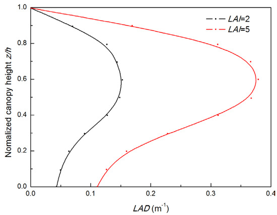
Figure 1.
The vertical profile of LAD in the vegetation region (LAI = 2, 5).
2.4.3. Effect of Buoyancy Force
The heat generated by solar radiation can be effectively trapped within specific areas of industrial parks, resulting in variations in air density that cannot be disregarded in the model [30]. Vegetation canopies, building surfaces, and the ground absorb solar radiation and create temperature differences in their vicinity. However, the air density variation is much smaller around building surfaces and the ground compared to the one inside vegetation canopies according to the simulation results, so that the impact of building surfaces and the ground can be neglected. Therefore, this research primarily focuses on analyzing the buoyancy force inside and above vegetation canopies. In Fluent solver, instead of utilizing the Boussinesq approximation, air density is calculated based on temperature.
The LES equation for energy transportation should be included in the model, which can be written as follows:
where is temperature, is the thermal diffusivity, is the subgrid thermal flux, and is the external heat source. The heat flux from solar radiation is added to the term in Equation (12), which is expressed by
where is the solar radiation heat flux at the top height of the canopy, which can be calculated by using the solar load model in Fluent; is an extinction coefficient, which is 0.6; and is defined as follows:
The variation in air density inside the plant canopy can be attributed to the absorption of solar radiation heat flux, as follows:
where represents the air temperature (K) [31].
2.4.4. Dry Deposition Inside Vegetation Area
The deposition motion plays a crucial role in the dispersion of particle pollutants, while it is negligible in gas flow dynamics. The particles are deposited and removed from the flow field when they come into contact with a surface and are trapped near the wall space. However, solid components are excluded from the canopy model described in Section 2.4.1, necessitating the application of a dry deposition model within vegetation areas. The key aspect of predicting particulate pollutant dispersion lies in calculating the deposition velocity [32]. In this study, we implemented the dry deposition model proposed by Petroff and Zhang [33], which demonstrates excellent agreement with field measurements.
The deposition velocity is dependent on the particle concentration and the density of the vegetation, which can be expressed by
Equation (16) is employed by incorporating user-defined functions into the particle motion equation to account for the deposition effect.
In conclusion, the presence of a vegetation barrier significantly influences the dispersion of particulate pollutants. The conditions of particles with and without canopy effects are illustrated in Figure 2. Without the canopy effect, particles are solely affected by gravity and drag forces from airflow, as described in Equation (9). However, upon entering the vegetation area depicted in Figure 2b, a block effect occurs due to the drag effect on the wind flow discussed in Section 2.4.2, resulting in horizontal deceleration of particles. To account for deposition effects, an additional body force is incorporated into Equation (9) causing particles to deposit at a speed of within the canopy. Moreover, the buoyancy effect needs to be taken into account under unstable meteorological conditions with solar radiation heating inside the canopy. In such circumstances, varying air densities lead to upward airflow trends that counteract deposition effects.
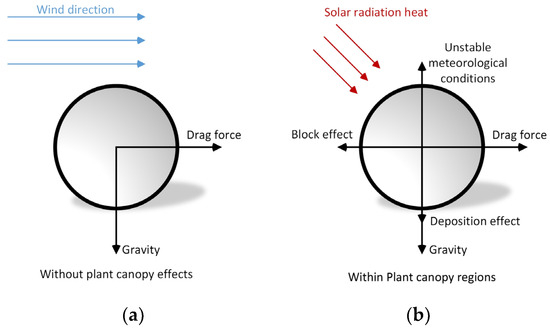
Figure 2.
The conditions of particulate pollutant without (a) and within (b) canopy effect.
2.4.5. Model Validation
The numerical simulations in this study were conducted using the Fluent solver. The effects of drag and buoyancy forces were applied to the wind flow stream, while the deposition effect was considered for particulate pollutants under various unstable meteorological conditions within the computational domain. User-defined functions compiled for the wind flow stream were validated by comparing them with verified data from previous studies by Shaw et al. [34] and Gu et al. [31]. The validation diagram, shown in Figure 3a, used a computational domain of 160 m × 60 m × 60 m, which is identical to that used in [31,34]. The canopy height was set at 20 m, horizontally uniform, and more detailed settings can be found in the previous research of Ma et al. [35]. Three typical cases with the same inlet velocity and solar radiation heat flux as those in [31,34] were calculated and the time-averaged wind velocity distributions on vertical profiles under different meteorological conditions are presented in Figure 3b. It can be seen that the simulation data show good agreement with the ones in previous research. The velocity increases under 5 m height and then it drops due to the block effect by the high-LAD canopy. The minimum value appears at where the LAD reaches its maximum value. Velocities follow an exponential distribution pattern above the canopy area where . Under unstable meteorological conditions, buoyancy force effects are taken into account, horizontal velocities are slightly influenced by upstream flows, and this influence enhances with the increase in meteorological instability. The slight discrepancy between this study and previous research is caused by the differences in boundary conditions. The wall shear stress is not calculated so that it can slightly influence the wind flow velocity above the ground. The numerical model utilized to investigate the impact of dry deposition was proposed by Petroff and Zhang [33], see Equation (16), which is employed to calculate the particle’s dry deposition velocity, is implemented using user-defined functions. Steffens et al. [25] applied this model to examine the influence of vegetation barriers on particle size distribution in a near-road environment, demonstrating favorable agreement with field measurements. In conclusion, the results in this study are in good agreement with previous works, showing that this canopy model is capable of simulating the distribution of the wind field and pollutants; therefore, it can be applied to the simulation of the industrial park.
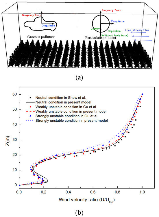
Figure 3.
(a) Schematic diagram of computational domain of model validation and (b) comparisons of time-averaged velocity distributions in vertical direction among this research and previous studies under various meteorological conditions [31,34].
2.5. Numerical Setup and Simulations
2.5.1. Computational Domain and Grid Generation
Numerical investigations were conducted to analyze the wind flow field and dispersion of particulate pollutants under various meteorological conditions in Nanjing Sample Industrial Park, located in the Qixia district of Nanjing, China. Figure 4a shows an aerial view of the industrial park, while Figure 4b depicts the computational domain with dimensions of 900 m × 800 m × 180 m. Zone “A” is an area with frequent human activities, where vegetation and buildings are marked. The building arrays are situated in the central area of the domain surrounded by streets on the west, north, and east sides so that the wind turbulence flow can be fully developed and not affected by the boundary walls. Vegetation areas are labeled in green color with a 10 m high canopy. The regions of herbage, which are mainly in the southwest of the domain, are neglected due to the slight influence on the wind flow and contaminant dispersion. Particulate pollutants originate from a source area during production processes, indicated by red color labeling. This source is positioned westward relative to the central building arrays and poses a potential threat to human health within the industrial park when influenced by westerly winds. Consequently, a wind flow inlet is established at the western boundary of the computational domain.
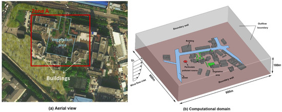
Figure 4.
(a) The aerial view of the industrial park, (b) Schematic diagram of computational domain.
In the vertical direction, the domain is divided into two regions: below 60 m high with tetrahedral unstructured grids exhibiting high-resolution meshes to accurately simulate wind flow within complex distributed building arrays (as shown in Figure 5a), and above 120 m high with hexahedral structured grids where wind flow behavior is less intricate and pollutant dispersion is not a significant concern, allowing for relatively sparse meshes. To ensure an accurate representation of flow fields within building arrays, Tominaga et al. [36] proposed a criterion stating that at least 10 grid nodes should be generated on each building surface. Accordingly, mesh refinement is applied to the areas adjacent to buildings as depicted in Figure 5c.
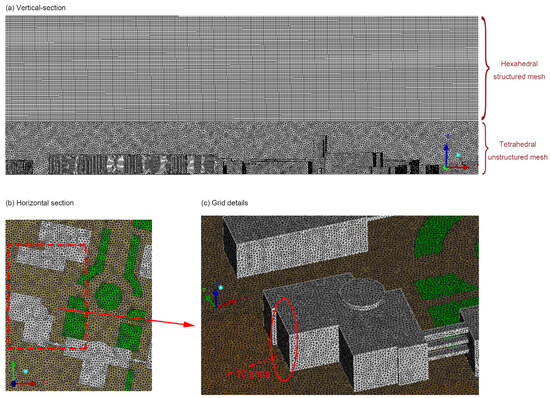
Figure 5.
The hybrid grid scheme of the domain: (a) Vertical section, (b) Horizontal section, and (c) Grid details.
Moreover, grid independence tests were conducted on three grid systems of 6 million, 9 million, and 12 million, as depicted in Figure 6. The comparison of pollutant concentrations was performed downwind from the source location within building arrays. Minor distinctions were observed in the simulation results, leading to the adoption of the 9-million-grid system to strike a balance between accuracy and efficiency. In conclusion, this combined grid system not only accurately calculates wind flow fields and contaminant dispersion but also enables a prompt response to harmful pollutants spreading in the central area of the industrial park.
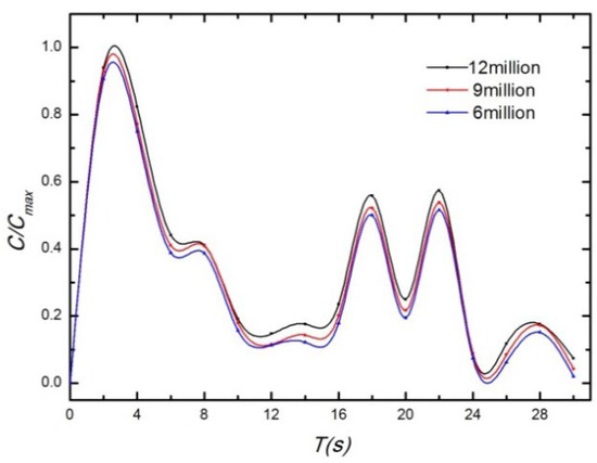
Figure 6.
The grid independency test by comparing the variation in pollutant concentration in the cases of 6-, 9-, and 12-million grid systems.
2.5.2. Boundary Conditions
- (1)
- Wind flow inlet boundary
Due to the pollutant source being located in the industrial park, the velocity inlet boundary is positioned toward the west of the domain depicted in Figure 4b to simulate scenarios influenced by westerly winds. The mean magnitude of velocity increases with height, conforming to a power law relationship as follows:
where is the wind velocity at the reference height, and is the exponential coefficient.
Moreover, the fluctuations in inflow play a crucial role in accurately simulating turbulent flow within atmospheric motions, particularly during unstable meteorological conditions. In the LES model, the spectral synthesizer provides a method of generating fluctuating velocity components based on the random flow generation technique that was proposed by Smirnov et al. [37]. This method is adopted in the research and validated with parameters of standard models in Section 3.1.
- (2)
- Outflow boundaries
The western boundary of the domain is considered an inlet for wind flow, while the eastern, northern, and southern boundaries are treated as outflow boundaries. In this configuration, a zero-diffusion flux of flow variables is imposed on the outflow boundary, which is commonly employed in fully developed turbulent flow scenarios. The escape boundary condition is applied to particulate pollutants at the outflow boundaries.
- (3)
- Building walls and ground
The mesh refinement is performed at the wall surfaces for the preparation of the near-wall treatment. The wind speed must be zero at ground level and on building walls. In this study, the 1/7 power law function is employed to accurately estimate the wall shear stress in order to satisfy the near-surface conditions:
where A = 8.3, B = 1/7; is the wall shear stress; is the wind velocity in the grid that is nearest to the wall; and is the distance from the grid center to the wall. The rebound condition is set to particulate pollutants on the building walls and ground.
- (4)
- Pollutant source
The chemical factories in Nanjing Sample Industrial Park emit particulate pollutants from the source, which can result in respiratory diseases. To simulate the dispersion and distribution of pollutants within the park, we designate the source as a velocity-inlet boundary. The particulate pollutant is injected into the domain with a concentration of 0.008 kg·m−2·s−1 at a velocity of 0.2 m/s. Further details regarding other parameters of the particulate pollutant are provided in the following Sections.
2.5.3. Computational Settings and Numerical Method
The computational settings of the simulation are presented in Table 2. The meteorological conditions are set to validate the turbulent characteristics of the atmospheric boundary layer in Section 3.1. The height of the atmospheric boundary layer and the exponential coefficient are influenced by the meteorological conditions; the specific correspondence will be described in the following discussion. LAI is set to 2 and 5 to represent the different densities of vegetation in winter and summer of Nanjing. Solar radiation heat flux is 800 W/m2 to represent a strongly unstable weather condition in summer daytime and 0 to represent a neutral condition at night. Sensitivity analysis is conducted by varying the density and diameter of the particulate pollutants.
Table 2.
LES-DPM simulation settings and parameters.
The finite volume method is employed in this simulation, and the coupling between pressure and velocity is processed using the SIMPLE algorithm. All simulation cases are conducted for a duration of 1800 s. During the simulation, the calculation of the gas phase continues for 600 s before commencing the injection of particulate pollutants. Both the time step for the gas phase and particle unsteady tracking model are set to 0.2 s.
3. Results and Discussion
3.1. Turbulent Characteristics of Atmospheric Boundary Layer
The specification method for defining fluctuations involves setting the turbulent kinetic energy and turbulent dissipation rate in the model. Turbulence intensity is employed to quantify the relative strength of fluctuating wind velocities, which can be defined as follows:
where is the fluctuating velocity and is the height of atmospheric boundary layer. Four simulation cases are established in Table 3 to validate the wind flow inlet boundary condition by comparing the vertical distribution of wind velocity and turbulent intensity. In Table 3, four cases are formed by arranging different daytime and meteorological conditions, and the season is assumed to be summer. The height of the atmospheric boundary layer and the exponential coefficient for each case can be obtained from local meteorological data in Nanjing, which are approximated. A minimum atmospheric boundary layer height of 500 m represents a neutral meteorological condition, while an increase in solar radiation intensity leads to an increase in this height. User-defined functions are utilized to incorporate vertical profiles of wind flow velocity, turbulent kinetic energy, and the turbulent dissipation rate on the inlet boundary into calculations. The results are presented in Figure 7.
Table 3.
Computational cases for analyzing turbulent characteristics of inlet boundary.
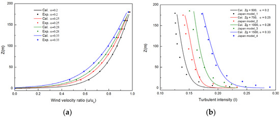
Figure 7.
The comparisons of (a) time-averaged wind velocity ratio between calculation results and exponential distributions, (b) turbulent intensity between calculation results and Japan models. = 0.2, 0.25, 0.28, 0.33; = 500, 750, 1000, 1500 m.
The time-averaged wind velocity and turbulent intensity are obtained at a distance of 50 m behind the inlet boundary, where the turbulence is fully developed. In Figure 7a, the wind velocity distributions under the four cases exhibit good agreement with the power law, indicating that the wind velocity inlet model can be applied across different daytime and meteorological conditions in Nanjing. The validation of turbulent characteristics at the inlet boundary is performed by comparing calculation data with measurement results from Uchida and Ohya [38] in Figure 7b, while maintaining consistent values for the atmospheric boundary layer height and exponential coefficient in all comparisons. The results reveal that the calculated data at the near-ground level area are smaller compared to the measured values, which can be attributed to assuming a non-slip condition at the ground level during simulation, whereas actual environmental conditions involve roughness near the ground, leading to increased turbulent intensity. The calculation data at high altitudes become closer to the measured values as the height of the atmospheric boundary layer and the exponential coefficient increase. Overall, under the four meteorological conditions considered here, differences between simulated data and measured values remain within an acceptable error of 15%. Consequently, it can be concluded that the wind flow inlet boundary condition accurately simulates turbulent flow in atmospheric boundary layers.
3.2. Effects of Meteorological Conditions on Wind Field
The wind field is a crucial factor influencing the dispersion and distribution of particulate pollutants in the industrial park, primarily influenced by meteorological conditions. Therefore, four representative cases were selected to calculate the wind field under different meteorological conditions in Nanjing, as presented in Table 4. The key variables considered include time of day, meteorological conditions, and season. The atmospheric instability is neutral, and the radiation heat flux is zero during nighttime. Two scenarios are examined: one with a heat flux of 800 representing a strongly unstable atmosphere and another with a heat flux of 200 representing a weakly unstable atmosphere. Additionally, the LAI is two in winter and five in summer. Other parameters such as the height of the atmospheric boundary layer Zg in Nanjing can be obtained from available meteorological data.
Table 4.
Computational cases for analyzing effects of meteorological conditions on wind field.
The wind field and pollutant distribution near the ground are closely associated with human health in the industrial park. Figure 8 illustrates the time-averaged wind fields at a height of 4 m for four different cases. Comparing Case 1 with Case 2, the velocity distribution appears to be similar. However, within the central area “A” of the industrial park as depicted in Figure 8a, there is a decrease in velocity due to a higher density of plant canopy in Case 2. Furthermore, solar radiation significantly influences the wind velocity distribution when comparing Case 2, Case 3, and Case 4 across the entire horizontal profile. Under unstable atmospheric conditions, overall wind velocities tend to be lower. Previous research by Ma et al. [35] indicates that under buoyancy effects caused by plant canopies and the presence of solar radiation, streamlines exhibit an upward trend vertically; additionally, there is an opposite wind direction observed between Case 2 and Case 3 within the northern region “A”. The near-ground wind fields become more uniform under unstable weather conditions.
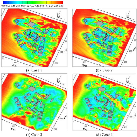
Figure 8.
The time-averaged wind field of four cases under different meteorological conditions: (a–d) represent Case 1–4 of different weather conditions, respectively. Unit: (m/s). Profile of H = 4 m.
It is critical to analyze the turbulent flow structures so LES is adopted in the study. Figure 9 illustrates the time-averaged vorticity magnitude and streamlines for Case 1, revealing significant vorticity concentrations on the leeward side of buildings, particularly within building arrays. By comparing Figure 9a,b, the vortex generation locations can be determined through an analysis of vorticity magnitude. In the central area “A” with plant canopy, a large vortex is generated here, which indicates that the complex turbulence structure in the canopy region is an important reason for the generation of vortices. Comparing Figure 9b with Figure 10a, it can be found that the accumulation of pollutants is closely related to the location of the vortex. The dispersion of particulate pollutants can be blocked by the vortices generated in the building arrays.
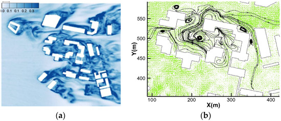
Figure 9.
The time-averaged vorticity magnitude (a) and streamlines in area “A” (b) of Case 1. Profile of H = 4 m.
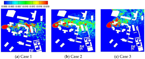
Figure 10.
The time-averaged concentration of particulate pollutants in central area “A” of industrial park: (a–c) represent Case 1–3, respectively. Unit: (kg/m3). Profile of H = 4 m.
3.3. Effects of Meteorological Conditions on Particulate Pollutant Distribution
The time-averaged concentration of particulate pollutants at H = 4 m in the central area of Case 1–3 is illustrated in Figure 10. The direction of pollutant dispersion is from west to east. In Case 1, where there is a slight drag effect from the plant canopy, pollutant accumulation is observed in the central area “A” and on the leeward side of the building arrays. Compared with Case 1, higher concentrations are found in area “A” while lower concentrations are observed on the leeward side of buildings in Case 2. This suggests that dense canopies effectively enhance particulate pollutant deposition and reduce downstream concentrations. In the sunny daytime of Case 3, the pollutant spreads to the northeast due to the buoyancy effect of the plant canopy. The direction of pollutant dispersion varies with changes in wind flow streamlines. The concentration is higher on the windward side of the plant canopy. The particulate pollutants inside the canopy regions can be removed from the ground to higher space when the buoyancy effect is larger than the deposition effect in strongly unstable weather conditions.
In the higher space, the dispersion of pollutants can be represented by iso-surfaces of concentration. Figure 11 illustrates four iso-surfaces in Case 1. The concentration is smaller in the higher region, and the dispersion of particulate pollutants exhibits the characteristics of smoke plumes. Only a small fraction of particles can traverse the canopy area and buildings, while the majority of pollutants tend to accumulate within the building array, and the environment outside the industrial park will not be damaged. The consideration of meteorological conditions and the utilization of the blocking effect of buildings are essential in order to effectively prevent the dispersion of air pollutants. Meanwhile, it is imperative to augment the canopy area within the industrial park in order to facilitate the effective removal and deposition of particles.

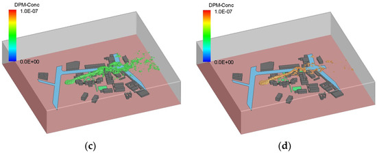
Figure 11.
The instantaneous iso-surfaces of particulate pollutant concentration in Case 1: (a) , (b) , (c) , (d) . Unit: (kg/m3).
In conclusion, the canopy is denser in summer and the leaf area index is larger. Consequently, the removal of particulate pollutants is more effective in canopy regions. In addition, the direction of pollutant dispersion can be changed due to the buoyancy effect and the pollutant can be partially removed when the meteorological condition is strongly unstable. The blocking effect of buildings and the deposition of the canopy can be used to reduce the influence of pollutants in different meteorological conditions.
3.4. Sensitivity Analysis
3.4.1. Deposition Effect
One of the distinctions between gaseous and particulate pollutant dispersion lies in the impact of deposition within the plant canopy. Figure 12 shows the time-averaged concentration distribution in area “A” with frequent human activities in Case 1; the data are obtained along the wind flow direction at H = 4 m. The canopy areas are marked within X = 192–208 m and X = 216–222 m.
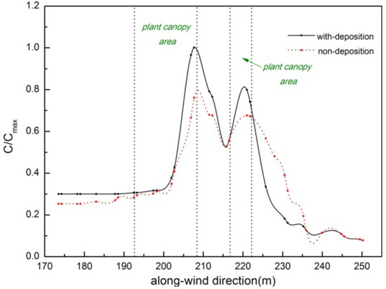
Figure 12.
The time-averaged concentration along wind direction of Case 1 at H = 4 m in area “A”. Black line: With deposition. Red line: Without deposition.
The concentration of pollutants increases upon entering the plant canopy area due to the drag effect on wind flow. Additionally, the deposition effect leads to an increased rate of concentration enhancement as shown by the black line in Figure 12. The concentration decreases after passing through the canopy and is found to be 50% lower than that on the windward side. This suggests that deposition plays a crucial role in removing particulate pollutants within the canopy area. However, it is essential to investigate further the relationship between deposition and buoyancy effects in future research.
3.4.2. Particle Density and Diameter
According to the Stokes formula, the deposition velocity of a particle is determined by its density and diameter. In this Section, we conduct sensitivity tests on these two parameters to investigate the impact of deposition effects in the simulations.
The time-averaged pollutant concentrations on the leeward of canopy of Case 4 in area “A” are shown in Figure 13. The particulate pollutant densities were set at 1200 and 2000 kg/m3 while keeping other parameters unchanged. It is evident that the concentration of pollutants with a density of 2000 kg/m3 is higher on the leeward side of the canopy. This difference is more pronounced within the height range of 2–10 m, indicating a greater deposition effect on high-density particles. The concentration of pollutants on the leeward side of the canopy exhibits an initial increase followed by a subsequent decrease within the vertical extent of the canopy. The maximum of LAD and pollutant concentration coincide at H = 6 m, indicating that the deposition effect is influenced by the LAD parameter. In Case 4, weak atmospheric instability results in the dominance of the deposition effect.
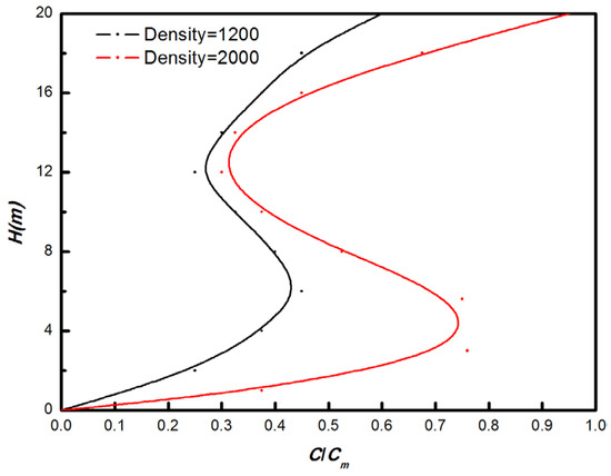
Figure 13.
The time-averaged concentration on the lee side of canopy of Case 4 in area “A”. Black line: Density = 1200 kg/m3. Red line: Density = 2000 kg/m3. The range of canopy H = 2–10 m.
The time-averaged concentrations on the leeward side of the canopy in Case 4 within area “A” are depicted in Figure 14 for particle diameters of 2.5, 5, and 10 . The density is set at 1200 kg/m3. Chemical factories emit numerous particles, including PM2.5 and PM10, which constitute the primary particulate pollutants in Nanjing’s atmosphere. The concentration of PM10 is much larger than that of PM2.5 near the ground, which indicates that the deposition effect is larger on the particles with a large diameter. Therefore, PM2.5 can spread further while PM10 can be blocked by the plant canopy easily.
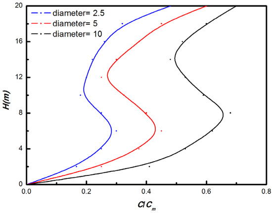
Figure 14.
The time-averaged concentration on the lee side of canopy of Case 4 in area “A”. Black line: Diameter = 10 . Red line: Diameter = 5 . Blue line: Diameter = 2.5 . The range of canopy H = 2–10 m.
4. Conclusions
The wind flow and particulate pollutant distribution inside Nanjing Sample Industrial Park under various meteorological conditions are investigated in this study by establishing a terrain model, LES-DPM model, and plant canopy model. Based on the results and discussion, the following conclusions can be drawn:
- To accurately set the inlet boundary condition, it is necessary to calculate both wind velocity and turbulent intensity profiles based on meteorological conditions. The two parameters are validated with standard data before the calculation of wind flow in the park.
- Four cases are simulated to analyze the effects of meteorological conditions; the wind filed can be blocked by a plant canopy, and it is completely changed when the buoyancy force is taken into account in unstable weather conditions and the wind field near the ground becomes uniform.
- The dispersion of pollutants is also influenced by meteorological conditions. In the presence of weather instability, the direction of pollutant dispersion shifts toward the northeast due to turbulent streamlines surrounding canopy regions, resulting in higher concentrations on the windward side of the plant canopies.
- The deposition effect of a plant canopy on particles plays a crucial role in the analysis of pollutant distribution. Under stable weather conditions, approximately 50% of particulate pollutants entering the canopy regions can be effectively removed. However, it is imperative to investigate the relationship between buoyancy and the deposition effect.
- The deposition effects are prominently observed on particles with high density and a large diameter. Additionally, the parameter LAD significantly influences the deposition process. In comparison to PM10, PM2.5 exhibits a lower deposition velocity, resulting in its wider dispersion both within and outside the industrial park.
- There are some approximate treatments and limitations in this research. For example, the leaf area index of different seasons in Nanjing Sample Industrial Park is processed approximately. The canopy regions are treated by the spatial averaging method, which is explained in Section 2.4.1. Weather conditions, wind velocities, and directions are not fully considered in this study. Some physical models need to be added for simulations under rainy or foggy conditions.
Author Contributions
The study was conducted with cooperation between all authors. The research was designed by W.Z. The modeling and simulations were conducted by X.M. The paper was written by X.M. and checked by W.Z. All authors have read and agreed to the published version of the manuscript.
Funding
This research was funded by Postgraduate Research and Practice Innovation Program of Jiangsu Province under Grant KYCX18_0083.
Institutional Review Board Statement
Not applicable.
Informed Consent Statement
Not applicable.
Data Availability Statement
The model validation data are available on the website http://dx.doi.org/10.1016/j.powtec.2016.08.062 (accessed on 28 August 2016). The meteorological data of Nanjing can be found on the website of the Nanjing Meteorological Bureau.
Conflicts of Interest
The authors declare no conflicts of interest.
References
- Liu, Y.; Yu, Q.; Huang, Z.; Ma, W.; Zhang, Y. Identifying Key Potential Source Areas for Ambient Methyl Mercaptan Pollution Based on Long-Term Environmental Monitoring Data in an Industrial Park. Atmosphere 2018, 9, 501. [Google Scholar] [CrossRef]
- Dockery, D.W.; Pope, C.A., III; Xu, X.; Spengler, J.D.; Ware, J.H.; Fay, M.E.; Ferris, B.G., Jr.; Speizer, F.E. An Association between Air Pollution and Mortality in Six U.S. Cities. N. Engl. J. Med. 1993, 329, 1753–1759. [Google Scholar] [CrossRef]
- Hong, Y.-J.; Huang, Y.-C.; Lee, I.-L.; Chiang, C.-M.; Lin, C.; Jeng, H.A. Assessment of volatile organic compounds and particulate matter in a dental clinic and health risks to clinic personnel. J. Environ. Sci. Health Part A 2015, 50, 1205–1214. [Google Scholar] [CrossRef]
- Liu, Y.S.; Miao, S.G.; Zhang, C.L.; Cui, G.X.; Zhang, Z.S. Study on micro-atmospheric environment by coupling large eddy simulation with mesoscale model. J. Wind. Eng. Ind. Aerodyn. 2012, 107–108, 106–117. [Google Scholar] [CrossRef]
- Finnigan, J. Turbulence in plant canopies. Annu. Rev. Fluid Mech. 2000, 32, 519–571. [Google Scholar] [CrossRef]
- Buccolieri, R.; Salim, S.M.; Leo, L.S.; Di Sabatino, S.; Chan, A.; Ielpo, P.; de Gennaro, G.; Gromke, C. Analysis of local scale tree–atmosphere interaction on pollutant concentration in idealized street canyons and application to a real urban junction. Atmos. Environ. 2011, 45, 1702–1713. [Google Scholar] [CrossRef]
- Bohrer, G.; Katul, G.G.; Walko, R.L.; Avissar, R. Exploring the effects of microscale structural heterogeneity of forest canopies using large-eddy simulations. Bound.-Layer Meteorol. 2009, 132, 351–382. [Google Scholar] [CrossRef]
- Boppana, V.B.L.; Xie, Z.-T.; Castro, I.P. Large-eddy simulation of dispersion from surface sources in arrays of obstacles. Bound.-Layer Meteorol. 2010, 135, 433–454. [Google Scholar] [CrossRef][Green Version]
- Bou-Zeid, E.; Overney, J.; Rogers, B.D.; Parlange, M.B. The effects of building representation and clustering in large-eddy simulations of flows in urban canopies. Bound.-Layer Meteorol. 2009, 132, 415–436. [Google Scholar] [CrossRef]
- Huang, J.; Cassiani, M.; Albertson, J.D. The effects of vegetation density on coherent turbulent structures within the canopy sublayer: A large-eddy simulation study. Bound.-Layer Meteorol. 2009, 133, 253–275. [Google Scholar] [CrossRef]
- Liu, Y.S.; Cui, G.X.; Wang, Z.S.; Zhang, Z.S. Large eddy simulation of wind field and pollutant dispersion in downtown Macao. Atmos. Environ. 2011, 45, 2849–2859. [Google Scholar] [CrossRef]
- Hanna, S.R.; Tehranian, S.; Carissimo, B.; Macdonald, R.W.; Lohner, R. Comparisons of model simulations with observations of mean flow and turbulence within simple obstacle arrays. Atmos. Environ. 2002, 36, 5067–5079. [Google Scholar] [CrossRef]
- Wang, X.; McNamara, K.F. Evaluation of CFD simulation using RANS turbulence models for building effects on pollutant dispersion. Environ. Fluid Mech. 2006, 6, 181–202. [Google Scholar] [CrossRef]
- Steffens, J.T.; Heist, D.K.; Perry, S.G.; Zhang, K.M. Modeling the effects of a solid barrier on pollutant dispersion under various atmospheric stability conditions. Atmos. Environ. 2013, 69, 76–85. [Google Scholar] [CrossRef]
- Xie, X.; Huang, Z.; Wang, J.; Xie, Z. The impact of solar radiation and street layout on pollutant dispersion in street canyon. J. Affect. Disord. 2005, 40, 201–212. [Google Scholar] [CrossRef]
- Chaisri, P.; Ponpesh, P. Prediction of PM2.5 Dispersion in Bangkok Pathumwan District) Using CFD Modeling. Eng. J. 2022, 26, 1–13. [Google Scholar] [CrossRef]
- Meng, M.-R.; Cao, S.-J.; Kumar, P.; Tang, X.; Feng, Z. Spatial distribution characteristics of PM2.5 concentration around residential buildings in urban traffic-intensive areas: From the perspectives of health and safety. Saf. Sci. 2021, 141, 105318. [Google Scholar] [CrossRef]
- Zhang, K.M.; Wexler, A.S. Evolution of particle number distribution near roadways—Part I: Analysis of aerosol dynamics and its implications for engine emission measurement. Atmos. Environ. 2004, 38, 6643–6653. [Google Scholar] [CrossRef]
- Sagaut, P.; Lee, Y.-T. Large Eddy simulation for incompressible flows: An introduction. Scientific computation series. Appl. Mech. Rev. 2002, 55, B115–B116. [Google Scholar] [CrossRef]
- Reynolds, W.C. Computation of turbulent flows. Annu. Rev. Fluid Mech. 1976, 8, 183–208. [Google Scholar] [CrossRef]
- Erlebacher, G.; Hussaini, M.Y.; Speziale, C.G.; Zang, T.A. Toward the large-eddy simulation of compressible turbulent flows. J. Fluid Mech. 1992, 238, 155–185. [Google Scholar] [CrossRef]
- Smagorinsky, J. General circulation experiments with the primitive equations: I. The basic experiment. Mon. Weather Rev. 1963, 91, 99–164. [Google Scholar] [CrossRef]
- Germano, M.; Piomelli, U.; Moin, P.; Cabot, W.H. A dynamic subgrid-scale eddy viscosity model. Phys. Fluids A Fluid Dyn. 1991, 3, 1760–1765. [Google Scholar] [CrossRef]
- Lilly, D.K. A proposed modification of the Germano subgrid-scale closure method. Phys. Fluids A: Fluid Dyn. 1992, 4, 633–635. [Google Scholar] [CrossRef]
- Steffens, J.T.; Wang, Y.J.; Zhang, K.M. Exploration of effects of a vegetation barrier on particle size distributions in a near-road environment. Atmos. Environ. 2012, 50, 120–128. [Google Scholar] [CrossRef]
- Morsi, S.A.; Alexander, A.J. An investigation of particle trajectories in two-phase flow systems. J. Fluid Mech. 1972, 55, 193–208. [Google Scholar] [CrossRef]
- Gosman, A.D.; Loannides, E. Aspects of computer simulation of liquid-fueled combustors. J. Energy 1983, 7, 482–490. [Google Scholar] [CrossRef]
- Wang, H.; Takle, E.S.; Shen, J. Shelterbelts and windbreaks: Mathematical modeling and computer simulations of turbulent flows. Annu. Rev. Fluid Mech. 2001, 33, 549–586. [Google Scholar] [CrossRef]
- Thom, A. Momentum, mass and heat exchange of vegetation. Q. J. R. Meteorol. Soc. 1972, 98, 124–134. [Google Scholar] [CrossRef]
- Yang, L.; Qian, F.; Song, D.-X.; Zheng, K.-J. Research on urban heat-island effect. Procedia Eng. 2016, 169, 11–18. [Google Scholar] [CrossRef]
- Gu, Z.; Zhang, Y.; Lei, K. Large eddy simulation of flow in a street canyon with tree planting under various atmospheric instability conditions. Sci. China Technol. Sci. 2010, 53, 1928–1937. [Google Scholar] [CrossRef]
- Piskunov, V. Parameterization of aerosol dry deposition velocities onto smooth and rough surfaces. J. Aerosol Sci. 2009, 40, 664–679. [Google Scholar] [CrossRef]
- Petroff, A.; Zhang, L. Development and validation of a size-resolved particle dry deposition scheme for application in aerosol transport models. Geosci. Model Dev. 2010, 3, 753–769. [Google Scholar] [CrossRef]
- Shaw, R.H.; Schumann, U. Large-eddy simulation of turbulent flow above and within a forest. Bound.-Layer Meteorol. 1992, 61, 47–64. [Google Scholar] [CrossRef]
- Ma, X.; Zhong, W.; Feng, W.; Li, G. Modelling of pollutant dispersion with atmospheric instabilities in an industrial park. Powder Technol. 2017, 314, 577–588. [Google Scholar] [CrossRef]
- Tominaga, Y.; Mochida, A.; Yoshie, R.; Kataoka, H.; Nozu, T.; Yoshikawa, M.; Shirasawa, T. AIJ guidelines for practical applications of CFD to pedestrian wind environment around buildings. J. Wind Eng. Ind. Aerodyn. 2008, 96, 1749–1761. [Google Scholar] [CrossRef]
- Smirnov, A.; Shi, S.; Celik, I. Random flow generation technique for large eddy simulations and particle-dynamics modeling. J. Fluids Eng. 2001, 123, 359–371. [Google Scholar] [CrossRef]
- Uchida, T.; Ohya, Y. Large-eddy simulation of turbulent airflow over complex terrain. J. Wind. Eng. Ind. Aerodyn. 2003, 91, 219–229. [Google Scholar] [CrossRef]


Disclaimer/Publisher’s Note: The statements, opinions and data contained in all publications are solely those of the individual author(s) and contributor(s) and not of MDPI and/or the editor(s). MDPI and/or the editor(s) disclaim responsibility for any injury to people or property resulting from any ideas, methods, instructions or products referred to in the content. |
© 2024 by the authors. Licensee MDPI, Basel, Switzerland. This article is an open access article distributed under the terms and conditions of the Creative Commons Attribution (CC BY) license (https://creativecommons.org/licenses/by/4.0/).