Numerical Simulation of Urban Natural Gas Leakage Dispersion: Evaluating the Impact of Wind Conditions and Urban Configurations

Abstract

This study investigates the dispersion of natural gas leakages in urban environments under varying wind conditions (Beaufort levels 1, 2, and 6) and street layouts, with a focus on the implications for mobile leak detection at a height of 0.3 m above ground. Through numerical simulations, we analyze how urban canyons influence wind field and methane (CH₄) concentration distributions, highlighting the impact of wind speed and urban geometry on gas dispersion. The key findings indicate that urban structures significantly affect gas dispersion patterns, with higher wind speeds facilitating better dispersion and reducing the risk of high-concentration gas buildups. The study underscores the need to consider both meteorological conditions and urban design in enhancing gas leak detection and safety measures in cities. The results contribute to improving emergency response strategies and urban planning for mitigating the risks associated with gas leaks.

1. Introduction

Air pollution, a critical environmental concern, encompasses the risks associated with urban gas pipeline leaks. These incidents carry increasingly significant consequences due to their potential to cause major safety accidents. Recent events in Chinese cities have underscored the severity of such incidents. For example, a gas pipeline leak in Shenyang in October 2021 led to a tragic explosion, resulting in five fatalities [1]. Similarly, other incidents across China, including explosions in Hunan Province and Jiangsu Province, have highlighted the dangers posed by inadequate gas safety measures and monitoring systems [2,3]. Beyond the incidents in China, significant gas leak accidents have occurred globally, underscoring the universal challenge of gas safety. For instance, the Aliso Canyon gas leak in the United States from October 2015 through February 2016 released over 109,000 tons of methane, making it one of the worst environmental disasters in U.S. history [4]. Similarly, the Ghislenghien gas explosion in Belgium on 30 July 2004, serves as a poignant reminder of the dangers associated with natural gas leaks. This tragedy occurred when a high-pressure natural gas line was ruptured during construction activities, leading to an explosion that claimed 24 lives and injured 132 people, causing substantial property damage [5]. Such incidents, spanning different continents, highlight the critical need for advanced detection and simulation techniques to mitigate the risks of gas leaks and prevent future accidents.

In the rapidly urbanizing landscape of Chinese cities, managing the safety of gas pipelines presents a multifaceted challenge. For instance, different testing methods have been proposed to improve the accuracy of natural gas leak detection. Knobelspies et al. (2016) proposed the design, development, and characterization of a novel, low-cost, precise, and reliable gas sensor system for the detection of the most relevant gases occurring in natural gas and biogas, namely methane, carbon dioxide, and hydrogen sulfide [6]. Barriault et al. (2021) proposed using machine learning methods to enhance the sensitivity of methane and ethane mixed gas detection [7]. Aldhafeeri et al. (2020) reviewed recent developments and future perspectives of methane gas detection sensors [8].

The current urban gas pipeline inspection methods, including manual inspections and pressure drop techniques, often fall short of effectively detecting leaks, especially under complex urban conditions. This highlights the urgent need for more advanced and effective monitoring methods. To address these challenges, gas companies have started adopting mobile monitoring methods, including vehicle-mounted inspections. These methods primarily rely on sensors placed close to the ground to detect elevated concentrations of methane and ethane, key indicators of gas leaks. However, the effectiveness of these methods can be limited in terms of coverage and sensitivity, particularly in complex urban environments. One such advancement is ABB’s MobileGuard™, a mobile gas leak detection system. While MobileGuard™ represents a significant step forward in leak detection technology, it primarily informs the inspection teams about the general upstream location of a gas leak but lacks the capability to intelligently pinpoint the exact leak point, even when close to the pollution source [9]. Yan et al. (2022) compared the measurement effects of their self-made mobile natural gas detection device with those of ABB MobileGuard and Picarro G4302, finding that their system using TDLAS had a shorter response time and lower sensitivity [10]. Currently, most numerical simulation studies on natural gas leakage primarily focus on the vertical wind field and the distribution of natural gas concentration [9,10,11], leakage characteristics [12,13], pollutant dispersion under explosion accident conditions [14,15], and natural gas leakage scenarios in certain specific situations [16,17,18,19]. However, previous research has paid relatively little attention to the characteristics of natural gas leakage on detectable horizontal planes.

The capability of computational fluid dynamics (CFD) to predict wind fields and pollutant dispersion around buildings has been extensively studied and validated through various seminal works. Blocken and Carmeliet (2004) have provided foundational insights into the pedestrian-level wind environment, highlighting the critical role of building geometry in influencing wind flow patterns [20]. Tominaga and Stathopoulos (2013) reviewed the effectiveness of CFD in simulating near-field pollutant dispersion in urban settings, emphasizing the progress in modeling techniques and their applicability in urban planning [21]. The best practice guidelines by Franke et al. (2007) serve as an essential reference for conducting accurate CFD simulations, ensuring the reliability of predictions related to urban airflow and pollutant dispersion [22]. Furthermore, the comparative study by Xie and Castro (2009) on the application of LES and RANS methods offers valuable perspectives on the dynamics of turbulent flow over arrays of obstacles, akin to urban environments [23]. Salim et al. (2011) specifically compared RANS and LES approaches in the context of a street canyon, underscoring the nuanced capabilities of CFD in capturing complex flow phenomena crucial for urban air quality management [24]. Collectively, these studies demonstrate the robustness of CFD as a predictive tool for understanding and mitigating the impacts of urban infrastructure on wind fields and pollutant distribution.

The atmospherentricacies of atmospheric boundary layer simulations underscore the paramount importance of accurately capturing boundary conditions, particularly the interaction between the vertical gradient of potential temperature and turbulence, which serves as a fundamental determinant of atmospheric stability [25]. This relationship, wherein the gradient acts as a source or sink for turbulence based on its nature, plays a critical role in dictating the dynamics and stability of the atmospheric boundary layer [26]. A positive gradient, indicative of a stably stratified atmosphere, suppresses turbulence and results in more laminar flow, whereas a negative gradient, characteristic of unstable conditions, enhances turbulence through convective currents [27]. This dynamic interplay significantly influences weather patterns, pollutant dispersion, cloud formation, and the efficacy of renewable energy sources by dictating the extent of mixing and vertical motion within the atmospheric boundary layer. Consequently, the accuracy of boundary condition representation becomes crucial in atmospheric modeling, ensuring the reliability of weather forecasting, climate projections, and environmental management strategies. Understanding and integrating these complex interactions into models is essential for advancing our ability to predict atmospheric phenomena and develop effective responses to climatic and environmental challenges.

In this study, we examine the influence of urban street and alley configurations on natural gas dispersion under varying wind conditions at Beaufort levels 1, 2, and 6, focusing particularly on the critical height of 0.3 m above ground, which is vital for mobile leak detection systems. Through advanced numerical simulations, we analyze wind field and CH₄ concentration distributions to understand how different wind speeds and urban layouts affect pollutant dispersion near the ground. This integrated approach provides essential insights for optimizing mobile gas leak detection in urban environments, highlighting the need to consider both meteorological conditions and urban geometry in emergency planning and response strategies.

2. Materials and Methods

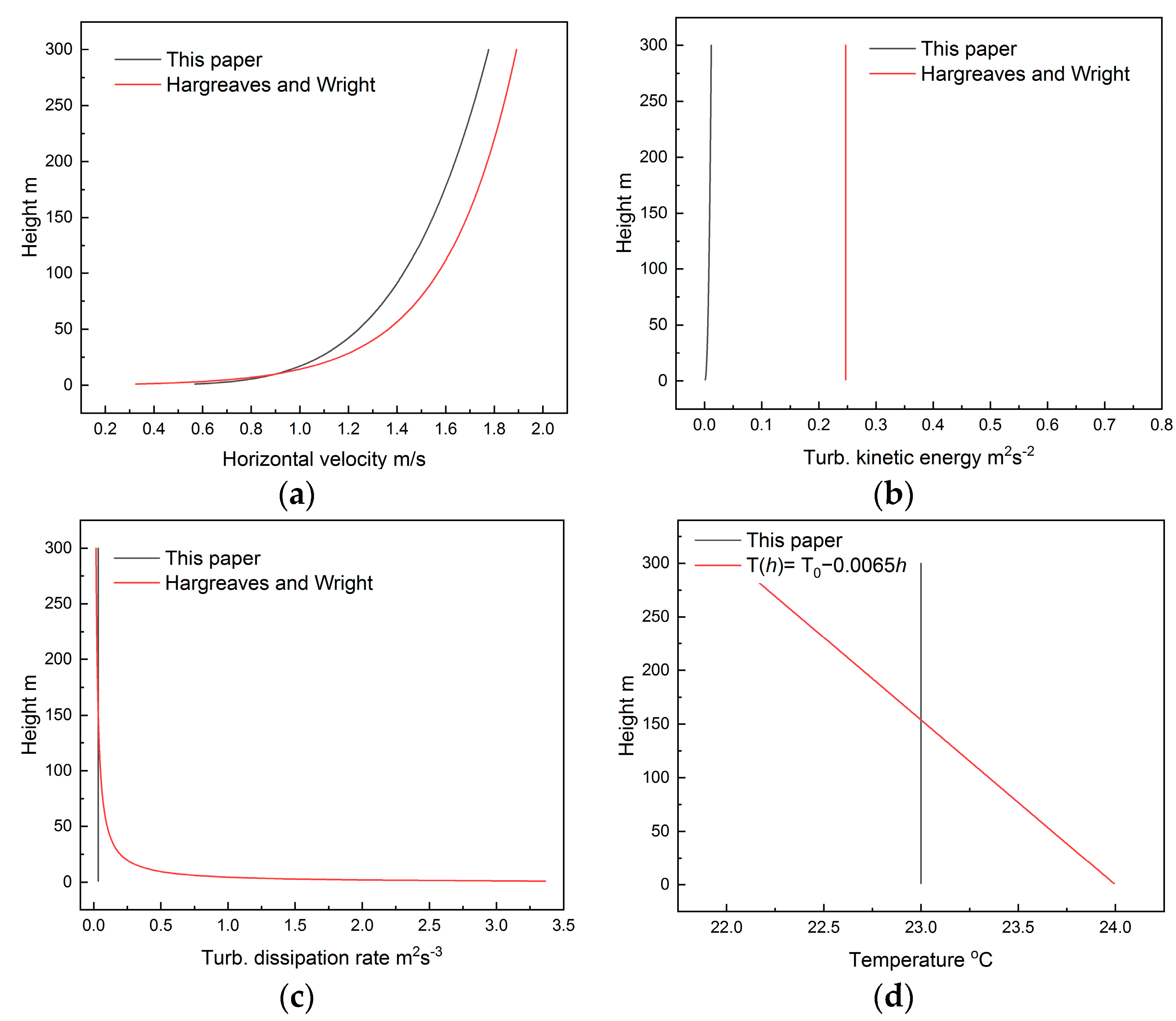
2.1. Governing Equations

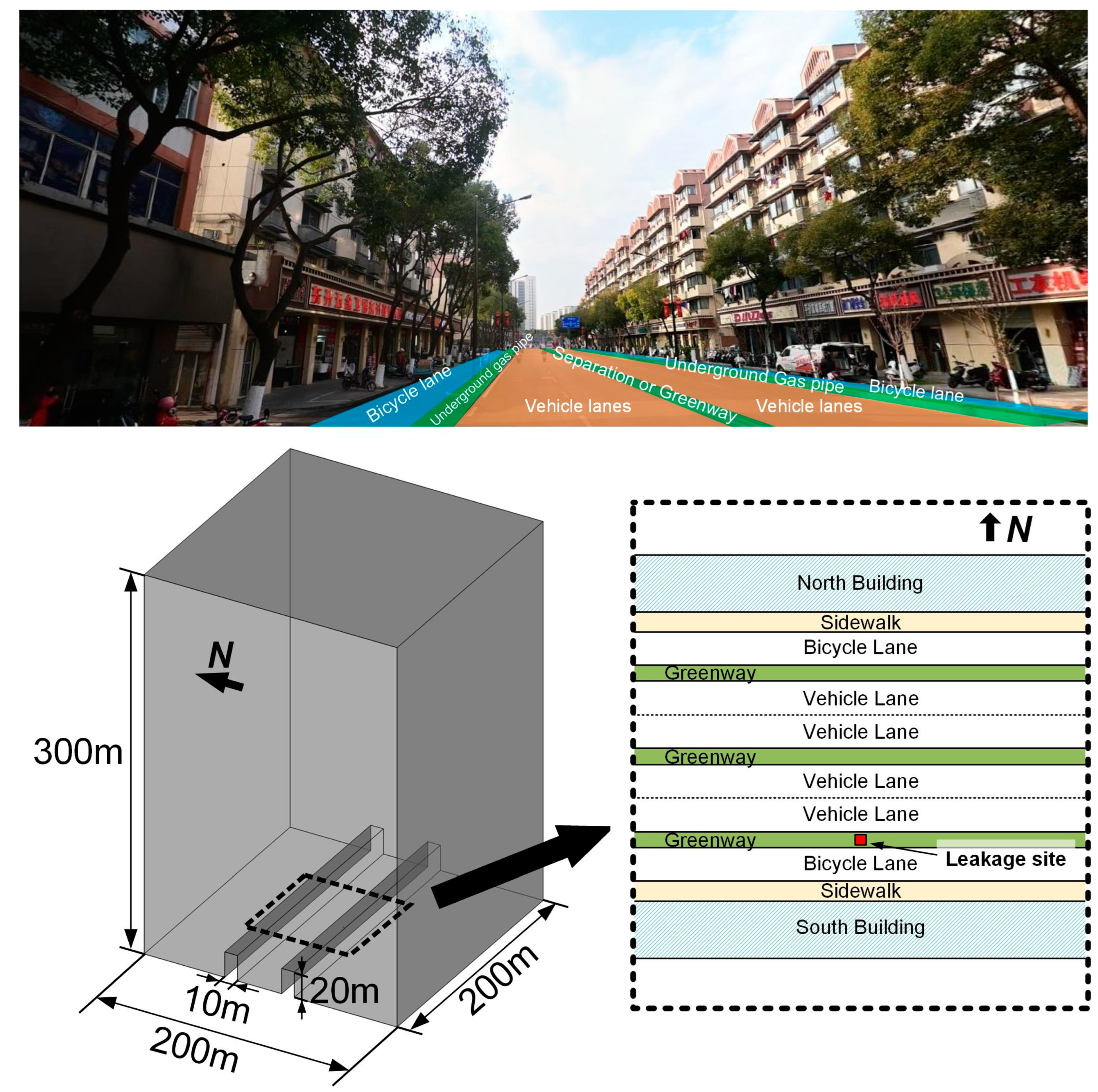
This paper employs the standard k-ε model for the simulation of the gas phase field [28]. The governing equations are as follows:

$$\frac{\partial }{\partial t}\left(\rho k\right)+\frac{\partial }{\partial x_i}\left(\rho k{u}_i\right)=\frac{\partial }{\partial x_j}\left[\left(\mu +\frac{{\mu }_t}{{\sigma }_k}\right)\frac{\partial k}{\partial x_j}\right]+G_k+G_b-\rho \epsilon$$

(1)

$$\frac{\partial }{\partial t}\left(\rho \epsilon \right)+\frac{\partial }{\partial x_i}\left(\rho \epsilon u_i\right)=\frac{\partial }{\partial x_j}\left[\left(\mu +\frac{{\mu }_t}{{\sigma }_{\epsilon }}\right)\frac{\partial \epsilon }{\partial x_j}\right]+C_{1\epsilon }\frac{\epsilon }{k}\left(G_k+C_{3\epsilon }{G}_b\right)-C_{2\epsilon }\rho \frac{{\epsilon }^2}{k}$$

(2)

where ρ is air density; k is the turbulence kinetic energy; u_i is velocity in i direction; ε is the dissipation rate of the turbulence kinetic energy; G_k and G_b are the generation terms of turbulence kinetic energy; μ_t is the turbulent viscosity; C_1ε, C_2ε, C_μ, σ_k, and σ_ε are experiment determined constants.

2.2. Domains

As shown in Figure 1, the typical street structure in the authors’ city of Nanjing features bidirectional lanes separated by separation or greenway, with green belts, bicycle lanes, and sidewalks located on the outside of the vehicle lanes. Five-to-seven-floor residential buildings or open spaces are located beyond the sidewalks. Natural gas pipelines are generally placed in the greenways between the vehicle and bicycle lanes. Based on routine inspection results, natural gas leaks mostly occur at the valves of underground gas pipelines, where valve pits are located. Thus, the street and alley scenario shown below Figure 1 was designed, assuming that natural gas leaks from a valve pit. The sampling position of the mobile natural gas leak detection device mounted on a vehicle is generally set at a height of 30 cm above the ground, so this study particularly focuses on the wind field and pollutant distribution near the ground.

In this research, the dispersion characteristics of natural gas leakage in typical ground-level urban environments are analyzed through simulations involving four prevalent urban street layouts with bidirectional quadruple-lane (two lanes in each direction) configurations. These scenarios encompass the following: Condition 1 (C1), characterized by the absence of buildings; Condition 2 (C2), where buildings are situated on the same side as the leakage source; Condition 3 (C3), with buildings located on the side opposite the leakage source; and Condition 4 (C4), featuring buildings on both sides of the leakage source. In the numerical simulations, if houses are present, they all face north–south. The dimensions of the buildings are shown in Figure 1. The dimensions of the computational domain for each scenario are set at 200 m by 200 m by 300 m.

Table 1. Simulation conditions table for different building structures, wind directions, and wind speeds.

Condition	Building Structure	Wind Directions	Beaufort Scale Levels
1	No building	South wind	1, 2, and 6
		East wind	1, 2, and 6
2	South building	South wind	1, 2, and 6
		East wind	1, 2, and 6
3	North building	South wind	1, 2, and 6
		East wind	1, 2, and 6
4	North and south buildings	South wind	1, 2, and 6
		East wind	1, 2, and 6

summarizes the detailed numerical simulation conditions.

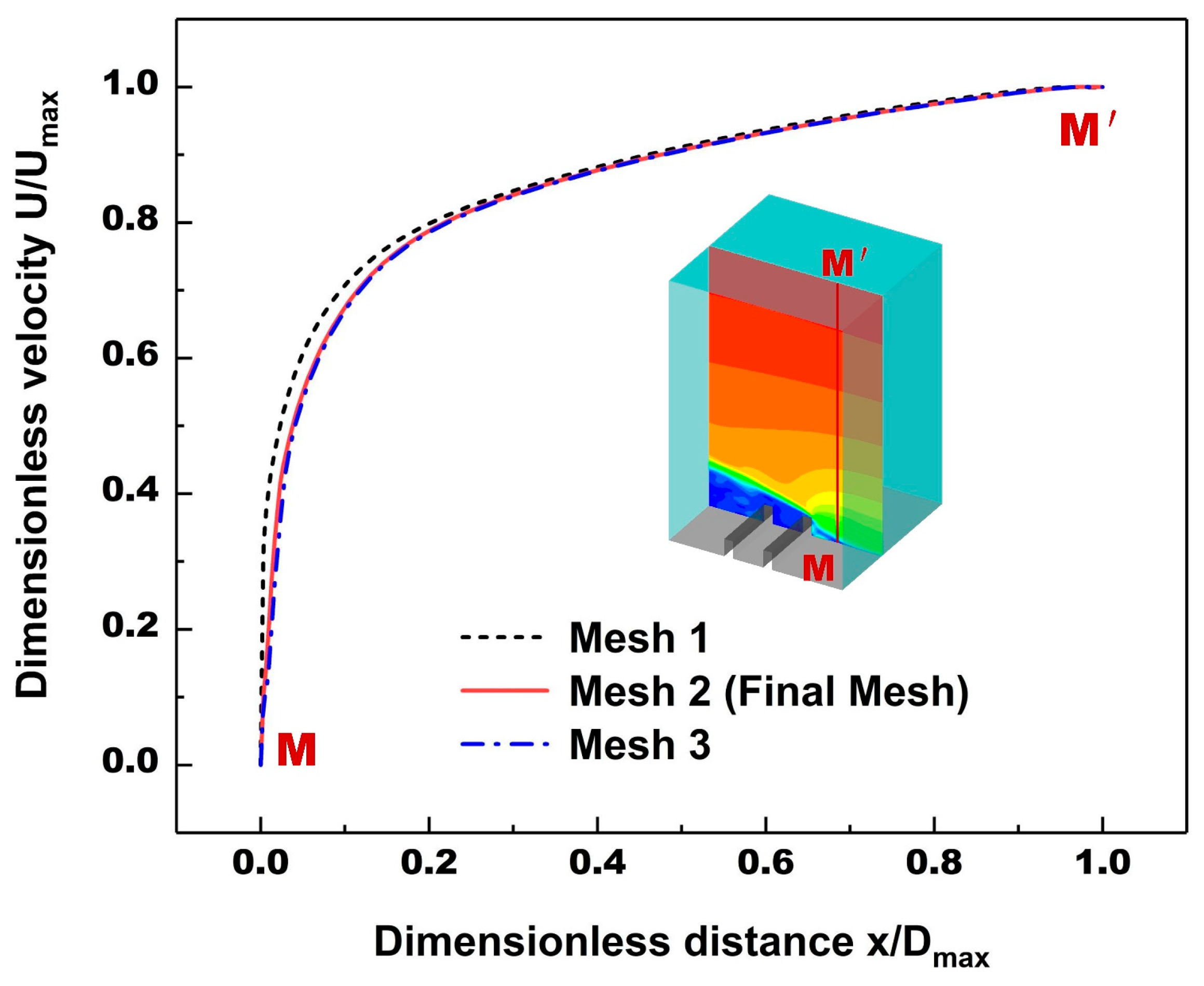
2.3. Numerical Setups

To investigate the distribution characteristics of natural gas leakages in the near-ground region, numerical simulations were conducted under south wind and east wind conditions at wind speeds corresponding to Beaufort scale levels 1, 2, and 6. Specifically, the wind speeds at a height of 10 m were 0.9 m/s, 2.4 m/s, and 11.8 m/s for Beaufort scale levels 1, 2, and 6, respectively. Steady-state numerical simulations were employed to model these scenarios. The wind speed at other heights can be determined based on the following equation [29]:

$$U_z={\left(\frac{z}{z_h}\right)}^{0.2}{U}_h$$

(3)

where U_z is the horizontal velocity at height z, and U_h is the velocity measurement at height h = 10 m. The inlet has a turbulence intensity of 10% and a temperature of 23 °C.

The mass flow rate of the leaked natural gas is 0.01 kg/s, with the mass ratios of CH₄, C2H6, and water vapor being 0.8557:0.0808:0.0635, respectively. The velocity of the gas at the leak source is 0.0224 m/s, which can be considered to have almost no impact on the local flow field. To reduce variables, it was assumed that the ambient temperature did not change. Convergence was considered achieved when the residual was less than 10⁻³.

To explore the pollutant distribution characteristics near the ground during natural gas leakage under different street and alley structures and wind directions, the flow field velocity distribution and CH₄ concentration distribution were obtained through three orthogonal planes passing the location of the leakage source. These planes include the north–south plane, the east–west plane, and the plane parallel to the ground at a height of z = 0.3 m, where the mobile leakage detection sensors are located.

The grids for all four scenarios have been validated for grid independence. For example, the dimensionless velocity distribution at the M-M’ location for Condition 4 under Beaufort level 2 south wind was compared across different mesh sizes, as shown in Figure 2. It was found that the difference between Mesh 2, with 2,143,465 cells, and Mesh 3, with 8,285,782 cells, was less than 5%, while Mesh 1, with 587,935 cells, had a significantly larger error. Therefore, Mesh 2 was chosen as the final simulation grid. Similarly, the mesh sizes for Conditions C1, C2, and C3 are 2,073,032, 2,133,867, and 2,136,580 cells, respectively. In this simulation, the y+ values on the windward side are generally between 30 and 200, but in some areas on the leeward side, y+ is less than 30. The surface roughness is 0.5 m. The outlet and the top of the simulation area are both set to zero-pressure outlet.

The grids for all four scenarios were validated for grid independence. For example, the dimensionless velocity distribution at the M-M’ location for Condition 4 under Beaufort level 2 south wind was compared across different mesh sizes, as shown in Figure 2. It was found that the difference between Mesh 2, with 2,143,465 cells, and Mesh 3, with 8,285,782 cells, was less than 5%, while Mesh 1, with 587,935 cells, had a significantly larger error. Therefore, Mesh 2 was chosen as the final simulation grid. Similarly, the mesh sizes for Conditions C1, C2, and C3 are 2,073,032, 2,133,867, and 2,136,580 cells, respectively. In this simulation, the y+ values on the windward side are generally between 30 and 200, but in some areas on the leeward side, y+ is less than 30. The surface roughness is 0.5 m. The outlet and the top of the simulation area are both set to zero-pressure outlet.

This article employs the conditions of the neutral atmospheric boundary layer and simplifies them. Figure 3 presents a comparison of horizontal wind speed, dissipation rate, and temperature variations with height under these simplified conditions at Beaufort scale level 1 against the neutral atmospheric boundary layer model [30].

3. Results

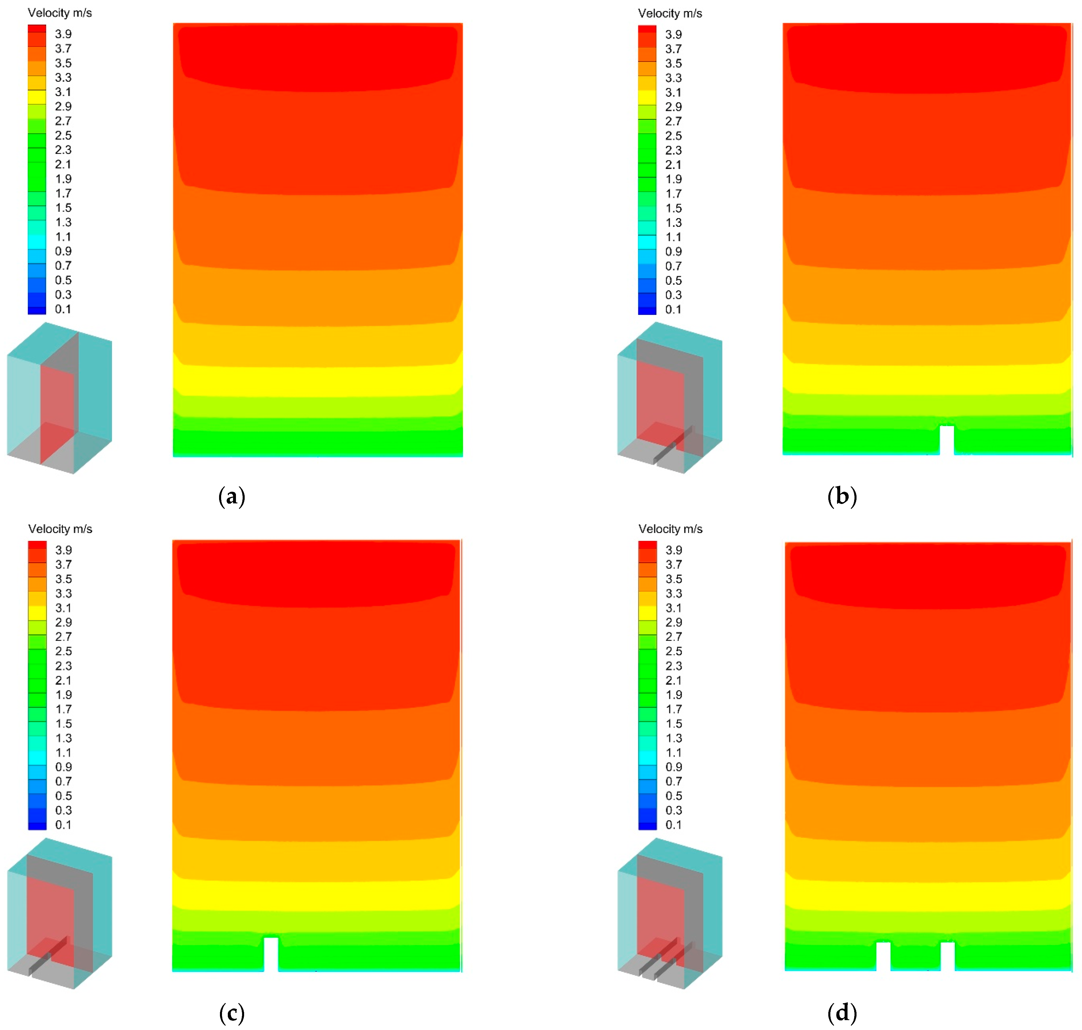
3.1. Canyon Structure Effect

Under Beaufort level 2 wind conditions, simulations were conducted for south and east wind scenarios to study the impact of canyon structures on the environmental wind field and pollutant dispersion distribution.

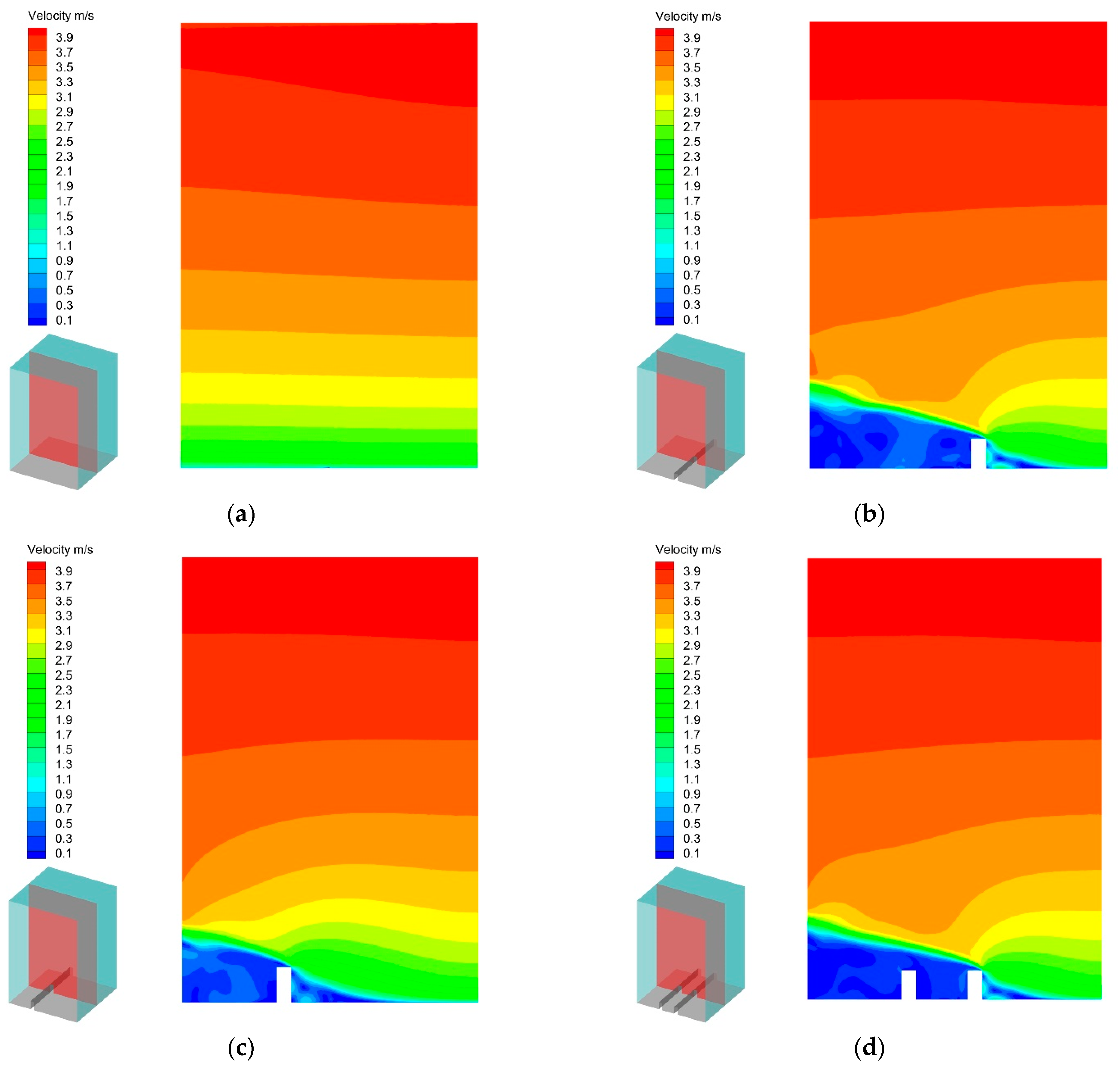
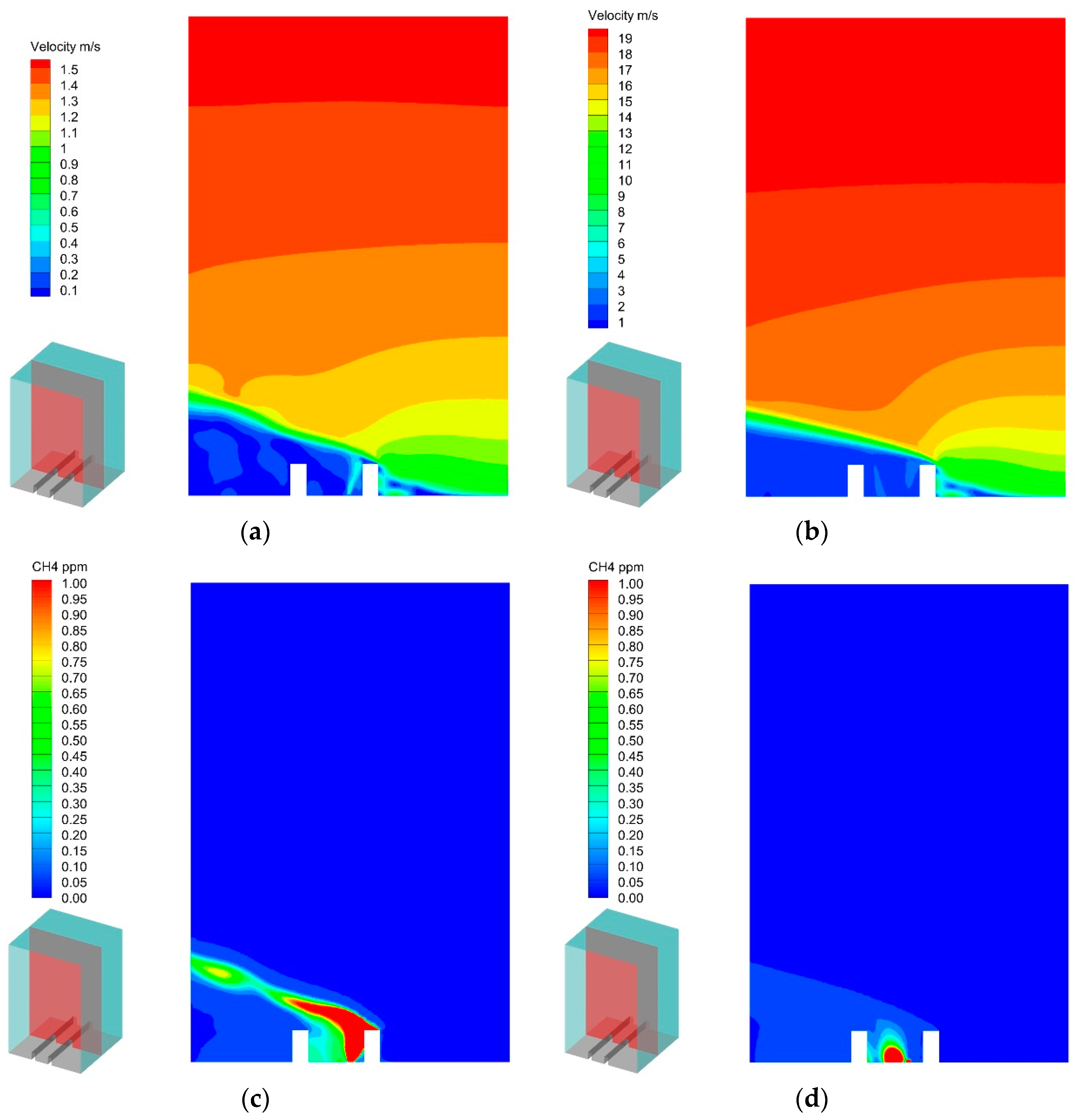
3.1.1. Wind Field Distributions under South Wind at Beaufort Level 2

Figure 4 below illustrates the wind field distribution at different vertical heights under the condition of a Beaufort level 2 south wind across various canyon configurations. Without buildings, the distribution of the wind field is largely unchanged, with little noticeable variation in vertical wind speed along the direction of airflow, except for a slight decrease in airflow speed at consistent heights along the flow direction. When canyons exist and are aligned perpendicular to the airflow direction, the vertical distribution of airflow speed depicted in Figure 4b–d shows certain similarities. A low-speed zone is observed forming in front of the first row of houses facing the wind, which forces the airflow upwards, and a larger low-speed zone behind the houses. Whether a second row of buildings is present does not significantly affect the flow field near the canyon. Similarly, observations for the vertical cross-sections in the east–west direction show similar results, with the velocity distribution behind the buildings in Figure 4f,h being quite close. Below the height of the buildings, it is generally a low-speed area, while Figure 4g, on the windward side of the buildings, presents some differences. However, near the ground, it remains a low-speed area, but with a rapid increase in wind speed with height.

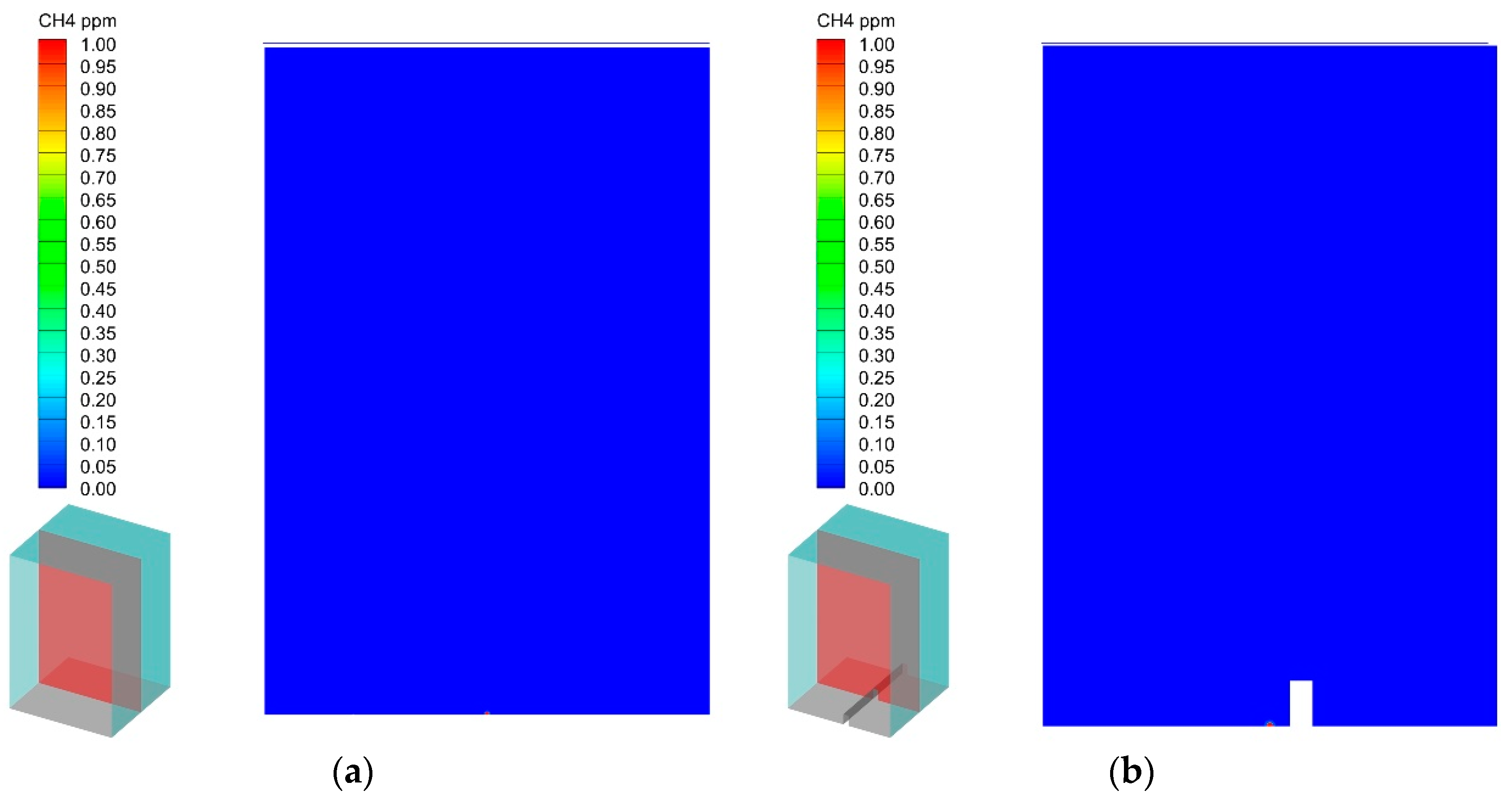
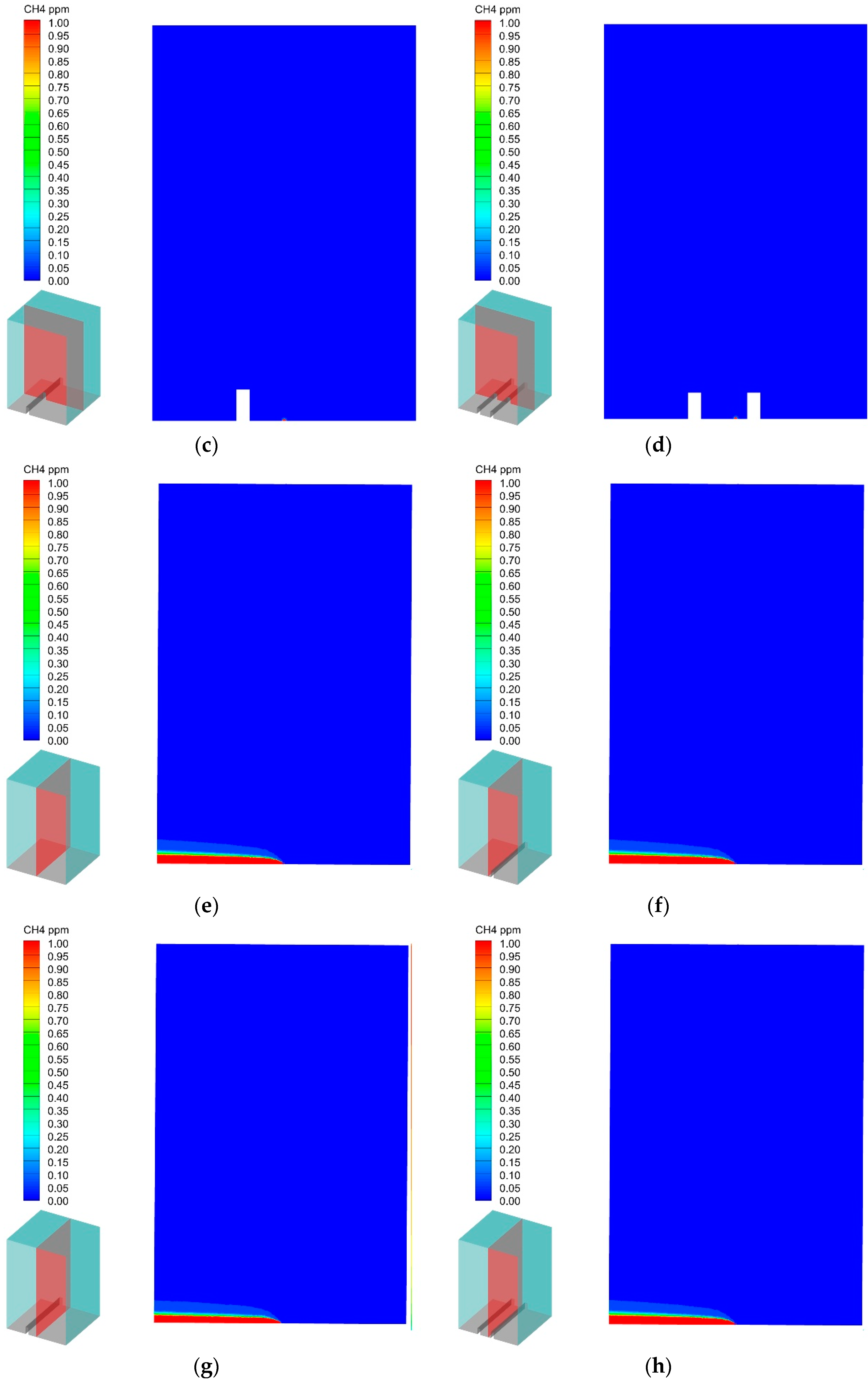
3.1.2. Pollutant Concentration Distribution under Beaufort Level 2 South Wind

Figure 5 illustrates the CH₄ distribution from a 1 m diameter circular natural gas leakage source under the wind direction conditions discussed in the previous section. It is evident that when there are no buildings on either side of the road, the dispersion of CH₄ is primarily along the flow direction, representing relatively good dispersion conditions. When buildings exist on either side of the street, as shown in Figure 5b–d,f–h, there is an obstruction to the dispersion of the natural gas leak. The dispersion effect is relatively better when the leakage source is upstream of the building, as shown in Figure 5c,g. Although the building obstructs the dispersion of natural gas, causing some accumulation on the street on the windward side of the building, the natural gas can still disperse downstream with the rising airflow. However, when the leakage source is on the leeward side of the building, as shown in Figure 5b,f, the air recirculating on the leeward side of the building causes natural gas to accumulate on the leeward side, creating a high concentration pollutant area near the leakage source. The worst dispersion conditions occur when buildings are present on both sides of the street, as shown in Figure 5d,h. Pollutants accumulate within the street until the natural gas can disperse upwards and be carried away by the airflow over the buildings. Therefore, the risk is greatest when buildings are present on both sides.

3.1.3. Wind Field Distribution under Beaufort Level 2 East Wind

Figure 6 shows the wind field distribution in the vertical direction under Beaufort level 2 east wind conditions across various canyon configurations. It is observed that when the distance between the canyons is relatively large, meaning the streets are wider, and the orientation of the buildings is roughly in alignment with the wind direction, there is little difference in the wind field distribution between scenarios with and without buildings on a macroscopic level. Except for a certain boundary layer effect near the buildings (as seen in Figure 6b–d), the velocity field distribution in sections along the flow direction at a certain distance from the houses (as seen in Figure 6f–h) is almost identical to that in the scenario without buildings (Figure 6e). There is a slight pressure loss along the flow direction, causing a minor reduction in flow velocity at the same height along the flow direction.

3.1.4. Pollutant Concentration Distribution under Beaufort Level 2 East Wind

Figure 7, similar to Figure 6, shows the pollutant concentration distribution in the vertical direction under Beaufort level 2 east wind conditions across various canyon configurations. Similar to the velocity field distribution discussed in the previous section, the pollutant concentration distribution also exhibits a high degree of similarity when the canyon widths are larger. In the north–south direction snapshots, pollutant distribution is visible only at the pollution source location as spot-like distributions, as shown in Figure 7a–d. In the east–west direction, which aligns with the airflow direction, it can be observed that the pollutant distribution under different canyon conditions, as shown in Figure 7f–h, is almost identical to the results in Figure 7e, where there are no buildings.

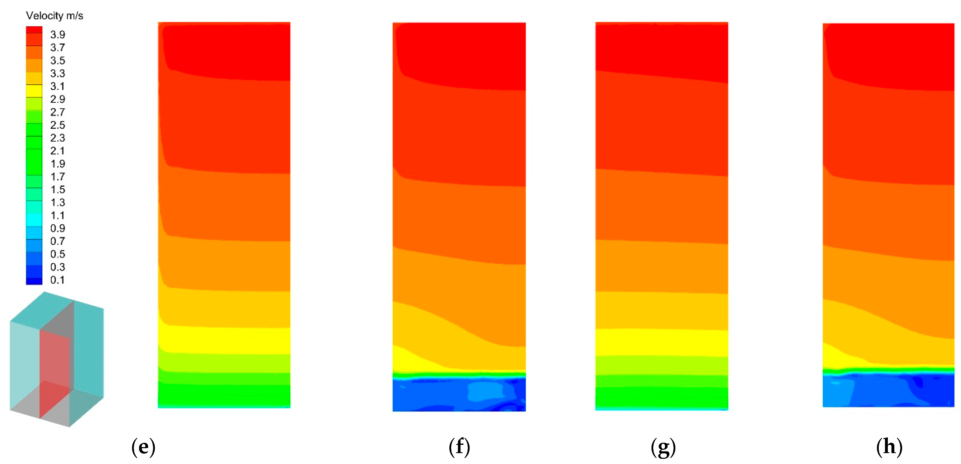
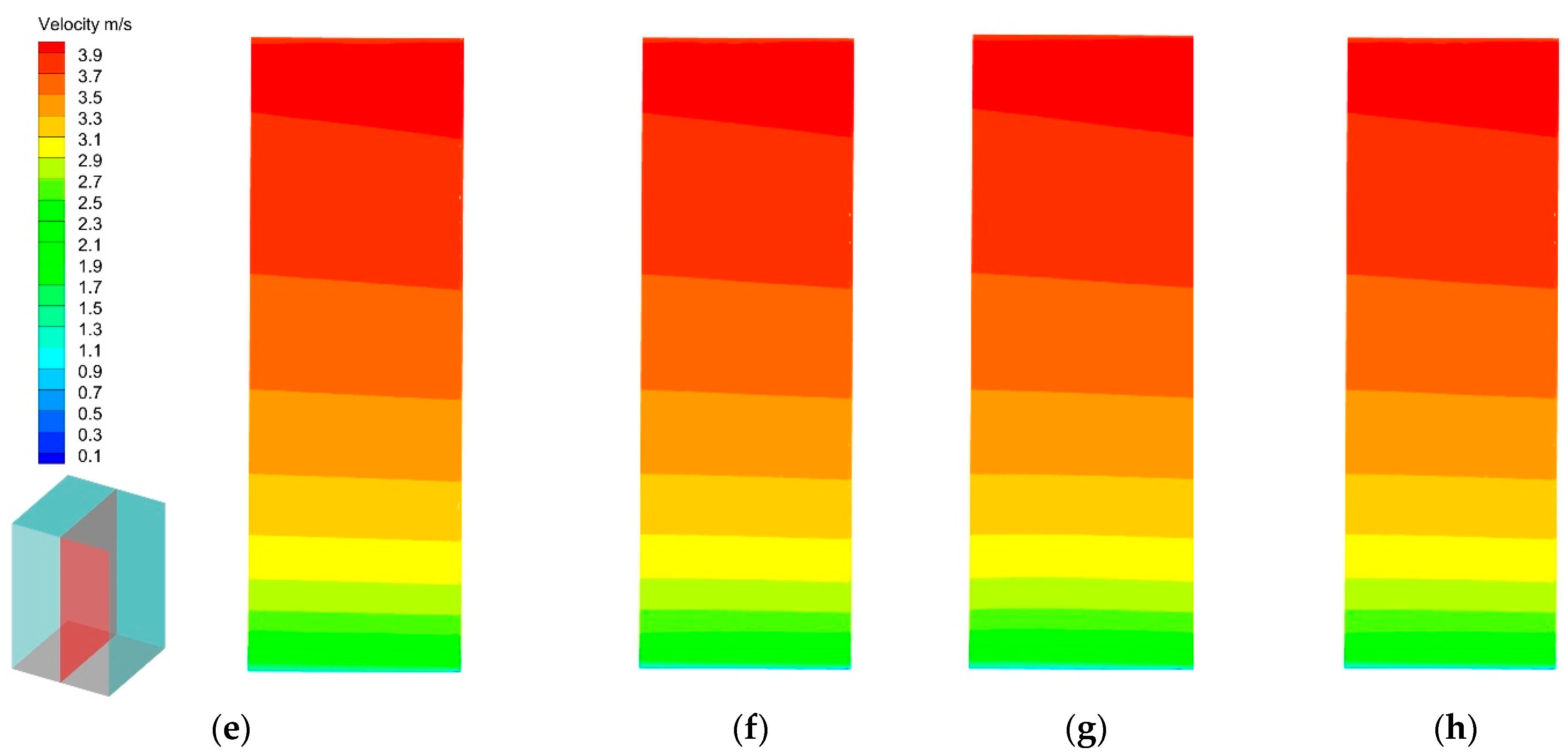
3.2. Wind Speed Effect

Clearly, wind speed has a significant impact on the velocity distribution of the environmental air and the concentration distribution of pollutants. Figure 8 shows the comparison of the air flow field distribution and CH₄ concentration distribution on both sides of the leak source at Beaufort levels 1 and 6 with buildings present. When wind speed increases significantly, as shown in Figure 8b, the contour of the low-speed zone behind the first row of buildings becomes more level, and the airflow speed is faster, thus enhancing the dispersion of pollutants. Therefore, in Figure 8d, CH₄ is less likely to accumulate behind the first row of houses but instead gradually disperses upwards and quickly dissipates with the airflow above the rooftops.

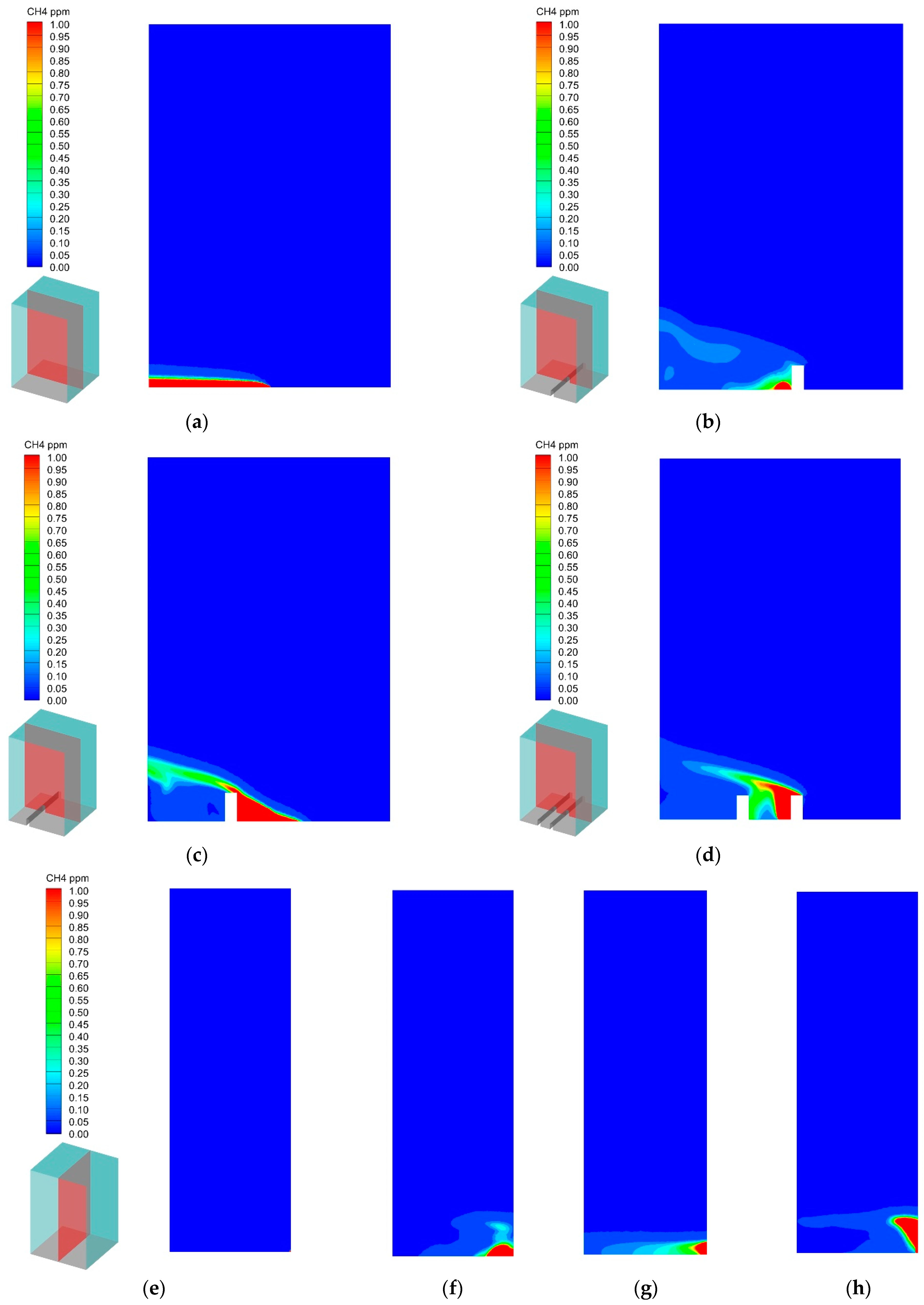
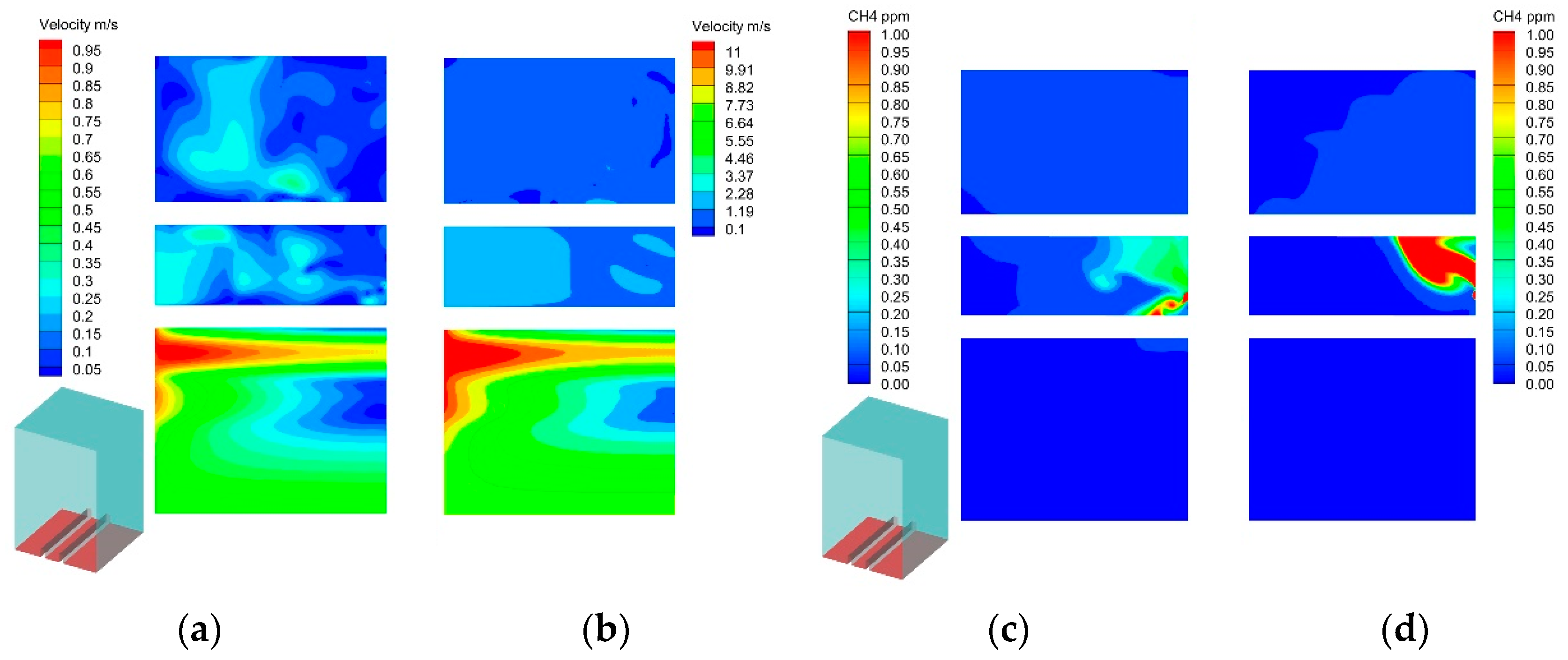
3.3. Near-Ground Pollutant Distribution under Different Conditions

The wind speed and pollutant concentration distribution near the ground have a significant impact on mobile natural gas leak detection. Therefore, the velocity distribution and pollutant concentration distribution at a height of 0.3 m above the ground were analyzed during the simulation process.

3.3.1. Near-Ground Pollutant Distribution under South Wind at Different Speeds

Figure 9 shows the velocity distribution near the ground under south wind conditions at Beaufort levels 1 and 6 (Figure 9a,b) and the pollutant concentration distribution (Figure 9c,d). Despite the apparent differences in the flow field and pollutant distribution in the vertical planes discussed in the previous section, near the ground, the flow field and pollutant distribution exhibit a certain similarity at different wind speeds. The concentration of CH₄ is higher near the pollution source, allowing for the identification of the pollution source location by searching for the area with the highest pollutant concentration or its symmetrical position during mobile tracing.

3.3.2. Near-Ground Pollutant Distribution under East Wind at Different Speeds

Figure 10 shows the velocity distribution near the ground under east wind conditions at Beaufort levels 1 and 6 (Figure 10a,b) and the pollutant concentration distribution (Figure 10c,d). At Beaufort level 1 east wind, the overall wind speed is lower, so the wind speed near the ground is even lower, making it more susceptible to the influence of the leaking gas. As a result, in Figure 10a, the flow speed downstream of the leak source is relatively increased. However, in Figure 10b, when the wind speed reaches Beaufort level 6, the airflow speed between two buildings is not significantly affected by the leak source. In Figure 10c, due to the slower air flow near the ground, the CH₄ gas moves upwards, resulting in a lower CH₄ concentration downstream. The concentration distribution in Figure 10d is similar to the results in Figure 6h under Beaufort level 2 east wind conditions, with a higher concentration of methane gas near the ground.

4. Conclusions

This study conducted a comprehensive analysis of natural gas leakage distribution characteristics in urban alley and street canyon structures under varying wind conditions, employing numerical simulations to understand the influence of wind direction and speed, as well as urban configurations, on gas dispersion. Our findings contribute to the field of urban safety and environmental engineering by offering insights into the near-ground distributions of leaked natural gas under different building structures and wind conditions. The key conclusions drawn from this research are as follows:

• This study identified unique pollutant distribution patterns associated with specific combinations of building structures and wind directions. Notably, when the wind is perpendicular to or parallel to buildings, pollutant dispersion exhibits distinctive characteristics that could potentially be used to predict the location of gas leaks. This insight paves the way for developing predictive models that utilize pollutant distribution data, along with wind conditions, to accurately locate leak sources.
• Our analysis shows that urban canyons, formed by buildings, have a profound effect on natural gas dispersion. Specifically, under a Beaufort level 2 south wind, gas tends to accumulate in low-speed zones behind buildings.
• Wind speed and direction are pivotal in determining the concentration and distribution of pollutants at ground level. Our findings reveal that higher wind speeds significantly improve natural gas dispersion, thereby minimizing the formation of high-concentration zones close to leak sources. This emphasizes the need for emergency plans and gas detection strategies to incorporate local meteorological data for enhanced effectiveness.

The main limitations of this article lie in the fact that using a power law for the vertical velocity profile is a simplified approximation, and the power utilized will depend on the atmospheric class. The text employs a neutral atmospheric boundary layer, for which a streamlined velocity profile differs from that of a realistic atmospheric flow. Additionally, the turbulence intensity, turbulence dissipation rate, and temperature variations with height are relatively minor in this article, differing somewhat from actual atmospheric conditions.

References

1. Explosion Equivalent to Approximately 80 kg of TNT, Cause of Shenyang Explosion Resulting in 5 Deaths Announced. Beijing Youth Daily, 16 January 2022. Available online: www.mem.gov.cn/xw/ztzl/2021/qgczrqaqpczz/pgt_4342/202201/t20220116_406772.shtml(accessed on 8 February 2024).
2. 13 Typical Accidents! Another Reminder for Gas Safety! Pengpai News, 4 July 2023. Available online: www.thepaper.cn/newsDetail_forward_23726572(accessed on 8 February 2024).
3. Ministry of Emergency Management of the People’s Republic of China. Urging to Profoundly Learn from Accident Lessons, Promoting the Strengthening and Implementation of Safety Responsibilities. 2 October 2021. Available online: www.mem.gov.cn/xw/yjglbgzdt/202110/t20211002_399521.shtml (accessed on 8 February 2024).
4. California Air Resources Board, Aliso Canyon Natural Gas Leak. 8 August 2018. Available online: https://ww2.arb.ca.gov/our-work/programs/aliso-canyon-natural-gas-leak (accessed on 26 March 2024).
5. The Brussels Times, Tribute to the Victims of the Ghislenghien Explosion, 12 Years on. 31 July 2016. Available online: https://www.brusselstimes.com/38501/tribute-to-the-victims-of-the-ghislenghien-explosion-12-years-on (accessed on 26 March 2023).
6. Knobelspies, S.; Bierer, B.; Perez, A.O.; Wöllenstein, J.; Kneer, J.; Palzer, S. Low-cost gas sensing system for the reliable and precise measurement of methane, carbon dioxide and hydrogen sulfide in natural gas and biomethane. Sens. Actuators B Chem. 2016, 236, 885–892. [Google Scholar] [CrossRef]
7. Barriault, M.; Alexander, I.; Tasnim, N.; O’Brien, A.; Najjaran, H.; Hoorfar, M. Classification and regression of binary hydrocarbon mixtures using single metal oxide semiconductor sensor with application to natural gas detection. Sens. Actuators B Chem. 2021, 326, 129012. [Google Scholar] [CrossRef]
8. Aldhafeeri, T.; Tran, M.-K.; Vrolyk, R.; Pope, M.; Fowler, M. A review of methane gas detection sensors: Recent developments and future perspectives. Inventions 2020, 5, 28. [Google Scholar] [CrossRef]
9. ABB. ABB Ability™ Mobile Gas Leak Detection System. 7 April 2021. Available online: https://new.abb.com/products/measurement-products/analytical/laser-gas-analyzers/advanced-leak-detection/abb-ability-mobile-gas-leak-detection-system (accessed on 8 February 2024).
10. Yan, G.; Zhang, L.; Zheng, C.; Zhang, M.; Zheng, K.; Song, F.; Ye, W.; Zhang, Y.; Wang, Y.; Tittel, F.K. Mobile Vehicle Measurement of Urban Atmospheric CH4/C2H6 Using a Midinfrared Dual-Gas Sensor System Based on Interband Cascade Laser Absorption Spectroscopy. IEEE Trans. Instrum. Meas. 2022, 71, 9509411. [Google Scholar] [CrossRef]
11. Liu, A.; Huang, J.; Li, Z.; Chen, J.; Huang, X.; Chen, K.; Xu, W.b. Numerical simulation and experiment on the law of urban natural gas leakage and diffusion for different building layouts. J. Nat. Gas Sci. Eng. 2018, 54, 1–10. [Google Scholar] [CrossRef]
12. Peng, S.; Li, C.; Liu, E.; Liao, K.; Wang, W.; Li, J. Numerical simulation of natural gas pipeline leakage. In Proceedings of the ICPTT 2011: Sustainable Solutions For Water, Sewer, Gas, and Oil Pipelines, Beijing, China, 26–29 October 2011; pp. 1502–1511. [Google Scholar]
13. Yang, J.; Zhang, J.; Mei, S.; Liu, D.; Zhao, F. Numerical simulation of sudden gas pipeline leakage in urban block. Energy Procedia 2017, 105, 4921–4926. [Google Scholar] [CrossRef]
14. Dezfouli, A.M.; Saffarian, M.R.; Behbahani-Nejad, M.; Changizian, M. Experimental and numerical investigation on development of a method for measuring the rate of natural gas leakage. J. Nat. Gas Sci. Eng. 2022, 104, 104643. [Google Scholar] [CrossRef]
15. Yuan, F.; Zeng, Y.; Khoo, B.C. A new real-gas model to characterize and predict gas leakage for high-pressure gas pipeline. J. Loss Prev. Process Ind. 2022, 74, 104650. [Google Scholar] [CrossRef]
16. Tong, S.; Li, X.; Ding, H.; Shuai, J.; Mei, Y.; Chan, S.H. Large-scale transient simulation for consequence analysis of hydrogen-doped natural gas leakage and explosion accidents. Int. J. Hydrogen Energy 2024, 54, 864–877. [Google Scholar] [CrossRef]
17. Cai, P.; Li, M.; Liu, Z.; Li, P.; Zhao, Y.; Zhou, Y. Experimental and numerical study of natural gas leakage and explosion characteristics. ACS Omega 2022, 7, 25278–25290. [Google Scholar] [CrossRef]
18. Zhou, K.; Li, F.; Cai, H.; Jing, Y.; Zhuang, J.; Li, M.; Xing, Z. Estimation of the natural gas leakage source with different monitoring sensor networks in an underground utility Tunnel: From the perspectives of energy security. Energy Build. 2022, 254, 111645. [Google Scholar] [CrossRef]
19. Bagheri, M.; Sari, A. Study of natural gas emission from a hole on underground pipelines using optimal design-based CFD simulations: Developing comprehensive soil classified leakage models. J. Nat. Gas Sci. Eng. 2022, 102, 104583. [Google Scholar] [CrossRef]
20. Blocken, B.; Carmeliet, J. Pedestrian wind environment around buildings: Literature review and practical examples. J. Therm. Envel. Build. Sci. 2004, 28, 107–159. [Google Scholar] [CrossRef]
21. Tominaga, Y.; Stathopoulos, T. CFD simulation of near-field pollutant dispersion in the urban environment: A review of current modeling techniques. Atmos. Environ. 2013, 79, 716–730. [Google Scholar] [CrossRef]
22. Franke, J.; Hellsten, A.; Schlünzen, H.; Carissimo, B. Best practice guideline for the CFD simulation of flows in the urban environment. In COST Action 732: Quality Assurance and Improvement of Microscale Meteorological Models; COST Office: Brussels, Belgium, 2007. [Google Scholar]
23. Xie, Z.-T.; Castro, I.P. LES and RANS for turbulent flow over arrays of wall-mounted obstacles. Flow Turbul. Combust. 2009, 82, 225–247. [Google Scholar] [CrossRef]
24. Salim, S.M.; Buccolieri, R.; Chan, A.; Di Sabatino, S. Numerical simulation of atmospheric pollutant dispersion in an urban street canyon: Comparison between RANS and LES. J. Wind. Eng. Ind. Aerodyn. 2011, 99, 103–113. [Google Scholar] [CrossRef]
25. Kahl, J.D.; Chapman, H.L. Atmospheric stability characterization using the Pasquill method: A critical evaluation. Atmos. Environ. 2018, 187, 196–209. [Google Scholar] [CrossRef]
26. Gryning, S.E.; Batchvarova, E.; Brümmer, B.; Jørgensen, H.; Larsen, S. On the extension of the wind profile over homogeneous terrain beyond the surface boundary layer. Bound. Layer Meteorol. 2007, 124, 251–268. [Google Scholar] [CrossRef]
27. Duynkerke, P.G. Application of the E–ε turbulence closure model to the neutral and stable atmospheric boundary layer. J. Atmos. Sci. 1988, 45, 865–880. [Google Scholar] [CrossRef]
28. Jones, W.P.; Launder, B.E. The prediction of laminarization with a two-equation model of turbulence. Int. J. Heat Mass Transf. 1972, 15, 301–314. [Google Scholar] [CrossRef]
29. Ma, X.; Zhong, W.; Feng, W.; Li, G. Modelling of pollutant dispersion with atmospheric instabilities in an industrial park. Powder Technol. 2017, 314, 577–588. [Google Scholar] [CrossRef]
30. Hargreaves, D.M.; Wright, N.G. On the use of the k–ε model in commercial CFD software to model the neutral atmospheric boundary layer. J. Wind Eng. Ind. Aerodyn. 2007, 95, 355–369. [Google Scholar] [CrossRef]
Figure 1. Schematic diagram of computational domain size, street and alley layout, and pollution source location.
Atmosphere 15 00472 g001
Figure 2. Grid independence test for C4.
Atmosphere 15 00472 g002
Figure 3. Comparison of the boundary conditions: (a) horizontal velocity, (b) turbulent kinetic energy, (c) dissipation rate, and (d) temperature.
Atmosphere 15 00472 g003
Figure 4. Wind field distribution along the height direction under Beaufort level 2 south wind in different canyon conditions: north–south direction (a) C1, (b) C2, (c) C3, and (d) C4; east–west direction (e) C1, (f) C2, (g) C3, and (h) C4.
Atmosphere 15 00472 g004aAtmosphere 15 00472 g004b
Figure 5. Pollutant distribution along the height direction under Beaufort level 2 south wind in different canyon conditions: north–south direction (a) C1, (b) C2, (c) C3, and (d) C4; east–west direction (e) C1, (f) C2, (g) C3, and (h) C4.
Atmosphere 15 00472 g005
Figure 6. Wind field distribution along the height direction under Beaufort level 2 east wind in different canyon conditions: north–south direction (a) C1, (b) C2, (c) C3, and (d) C4; east–west direction (e) C1, (f) C2, (g) C3, and (h) C4.
Atmosphere 15 00472 g006aAtmosphere 15 00472 g006b
Figure 7. Pollutant distribution along the height direction under Beaufort level 2 east wind in different canyon conditions: north–south direction (a) C1, (b) C2, (c) C3, and (d) C4; east–west direction (e) C1, (f) C2, (g) C3, and (h) C4.
Atmosphere 15 00472 g007aAtmosphere 15 00472 g007b
Figure 8. Comparison of wind field and CH4 concentration distributions at various heights in C4 configuration under south wind conditions at Beaufort levels 1 and 6: (a) wind field distribution at level 1; (b) wind field distribution at level 6; (c) CH4 concentration distribution at level 1; and (d) CH4 concentration distribution at level 6.
Atmosphere 15 00472 g008
Figure 9. Wind field and CH4 concentration distributions at 0.3 m above ground in C4 configuration under south wind conditions at Beaufort levels 1 and 6: (a) wind field distribution at level 1; (b) wind field distribution at level 6; (c) CH4 concentration distribution at level 1; and (d) CH4 concentration distribution at level 6.
Atmosphere 15 00472 g009
Figure 10. Wind field and CH4 concentration distributions at 0.3 m above ground in C4 configuration under east wind conditions at Beaufort levels 1 and 6: (a) wind field distribution at level 1; (b) wind field distribution at level 6; (c) CH4 concentration distribution at level 1; and (d) CH4 concentration distribution at level 6.
Atmosphere 15 00472 g010