Correlations between Urban Morphological Indicators and PM_2.5 Pollution at Street-Level: Implications on Urban Spatial Optimization

Abstract

During rapid urbanization, microclimate environment deterioration through events such as haze pollution and heat waves has continuously occurred in cities, which greatly affects the living environment, production activities, and health of urban residents. Therefore, it is particularly necessary to explore methods for controlling and optimizing the urban microclimate environment. In this paper, based on the mechanism of the effect of urban spatial structure at street-level on the distribution of atmospheric particulate matter, an indicator system that can be employed to comprehensively describe and quantify urban morphological structure at street-level was constructed from eight aspects: the spatial morphology of street-valleys, intensity of land use and development, geometric structure of buildings, inhomogeneity of buildings, roughness of the underlying surface, distribution of ecological landscapes, 3D architectural landscape morphology, and ventilation potential. Furthermore, using satellite remote sensing images and vector thematic maps of Shanghai, indicator factors were quantified by applying GIS technique. The intrinsic mechanism of the influence of the urban morphology on the diffusion and transport of atmospheric particulate matter was comprehensively analyzed by combining statistical methods and data mining algorithm, and eight key dominant factors were identified that can be considered to improve the urban ventilation conditions and help control urban air pollution, namely, the land use intensity, urban canopy resistance, vegetation cover, spatial congestion rate, comprehensive porosity, height-to-gross floor area ratio, building density, and average building volume ratio. As such, according to the quantitative analysis results for various combinations of the dominant factors, a spatial optimization strategy at street-level that can help improve the urban air quality was proposed in terms of identifying the pathways through which urban spatial elements affect the distribution of particulate matter, i.e., controlling the source–flow diversion–flow convergence process.

1. Introduction

China is currently experiencing a stage of rapid urbanization development characterized by population increase, land expansion, and changes in surface properties. Urbanization has profoundly impacted the local climate and environment, for example, the urban heat island effect, atmospheric pollution, and weakening of air exchange have become important issues that must be urgently resolved for ensuring the sustainable development of cities [1,2,3,4].

A large number of studies have proved that there is a significant influence between some factors in the process of urban development and the distribution of PM2.5 pollution, and it has been found that measures such as constructing a reasonable urban form, scientifically adjusting the density of the road network, the density of buildings, the proportion of the population, and upgrading the green space within the city [5] have a significant effect on the reduction in PM2.5 concentration. Studies on the impact of the urban morphological structure on the air quality have focused mainly on the architectural planning industry. Ref. [6] demonstrated that air pollution is closely related to various factors, such as the intensity of land use and development, layout of urban spatial structures, and transportation road networks. When exploring the influence of land use types on the distribution and dispersion of PM_2.5 in cities, the built-up green space, residential land, and cultivated land are the main research objects. Studies have shown that different green land landscape patterns affect the distribution of the PM_2.5 concentration [7]. It has also been reported [8] that increasing the vegetation cover in districts can effectively improve the air quality. Ref. [9] showed that green coverage contributes to a high degree of change in PM_2.5. Ref. [10] revealed that the size of the fallow forest area is related to the distribution of the PM_2.5 concentration.

Researchers have used street-level morphological indicators to study the relationship between the distribution of atmospheric pollutants concentration and the three-dimensional spatial structure of cities, usually. Ref. [11] investigated the volume, orientation, and plan layout of buildings and reported that the morphological structure of a building can impose different degrees of influences on the diffusion and transport of atmospheric particulate matter. In addition, indicators such as the standard deviation of the building height, average building height, and average building volume are highly correlated with the dispersion of air pollutants in high-density districts and neighborhoods [12]. Ref. [13] showed that the height and density of building complexes significantly affects the distribution of atmospheric particulate matter. Ref. [14] reported that the building density, building height, and building volume significantly affect PM_2.5. Ref. [15] recently showed that the building-to-volume ratio affects the distribution of the PM_2.5 concentration.

Many studies have focused on evaluating the correlation between the urban morphology and the distribution and dispersion of atmospheric particulate matter. Ref. [16] investigated the correlation between PM2.5 distribution and urban form parameters in a cold climate city in China using gradient boosted regression trees, and quantitatively analyzed the influencing factors and found that building density had a greater impact on PM2.5 concentration. However, research on the urban spatial morphology lacks a set of comprehensive quantitative analysis methods, which cannot be applied in the optimization of urban spaces. Therefore, from the perspectives of urban planning and design, statistical and data mining methods are adopted in this paper to identify the dominant factors and their combinations affecting the diffusion of atmospheric particulate pollutants, and the intrinsic mechanism through which the street-level morphology affects the distribution and diffusion of atmospheric particulate matter is revealed by constructing a model to quantify the indicator system of the urban morphology. Then, an indicator system applicable to urban space optimization is derived, and a set of urban space optimization design strategies based on various combinations of the dominant factors is proposed. Finally, several block space optimization design strategies are proposed based on different combinations of the dominant factors to provide a scientific basis and decision-making suggestions for the optimization of urban block space structures to improve the urban microclimate environment and provide a liveable and comfortable living environment for urban residents.

The study and visualization of the spatial and temporal distribution characteristics of PM2.5 pollution and its influencing factors are of reference value for the study of the diffusion, control, and prevention of PM2.5 pollution. Secondly, using scientific methods to systematically study the relationship between urban neighborhood morphology and PM2.5 concentration can help the government environmental protection department to carry out the renovation of old cities and the expansion of new cities in a more reasonable way according to the degree of pollution in different areas. Thirdly, we can better understand the characteristics of the urban morphology, explore the environmentally friendly urbanization mode, and provide a scientific basis for decision-making to improve the air quality as well as the rational urban planning.

2. Study Area and Materials

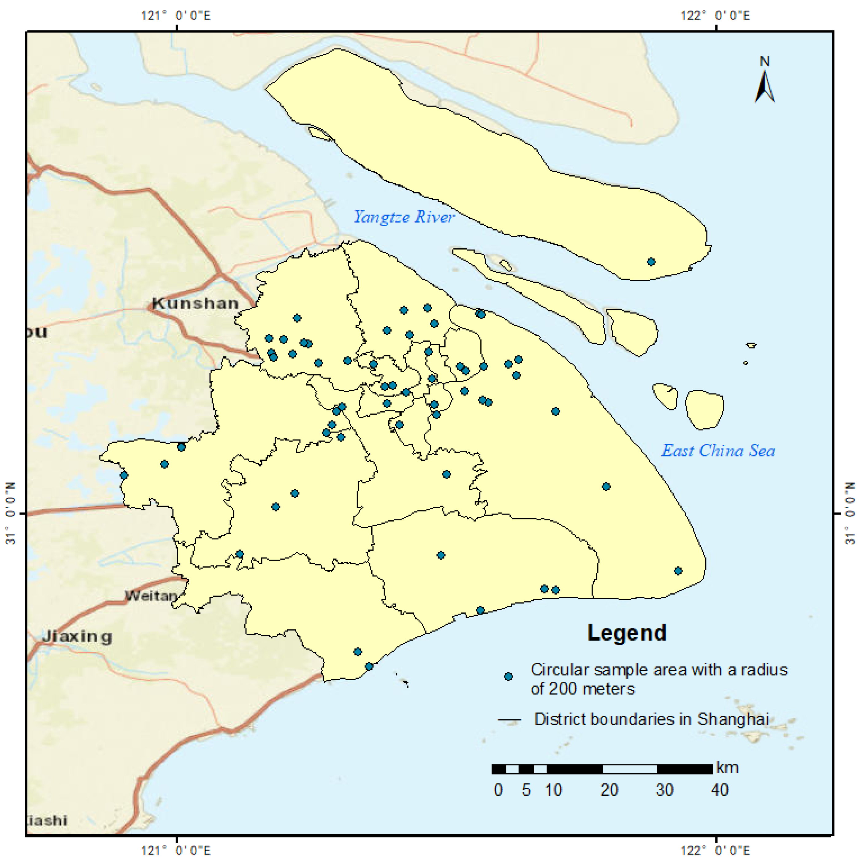
2.1. Study Area

Shanghai is located at longitudes 120°51′~122°12′ E and latitudes 30°40′~31°53′ N, with a total area of approximately 8239 km². The average elevation of Shanghai is approximately 4 m above sea level, and except for a few hilly mountain ranges in the southwestern part of the city, the terrain is flat, with a small relative altitude difference. Shanghai has a typical subtropical monsoon climate, with a significant difference in the dominant wind direction between summer and winter. Notably, the dominant wind directions in summer are east-northeast and north-northeast, and in winter, the dominant wind direction is north. Due to the limited land resources, Shanghai has gradually developed into the largest economic center and the largest industrial and commercial port city in China. As a high-density megacity, Shanghai can provide sufficient samples for the study of the urban morphology and atmospheric environment. In this paper, 60 sample districts were selected from the built-up areas in Shanghai (Figure 1). Ref. [17] studied the influence of the building forms and layout on the dispersion of air pollutants and showed that the concentration of pollutants at small area scales is slightly affected by more distant emission sources because districts and neighborhoods encompass complex spatial structures that can notably affect pollutant migration. Thus, in this paper, a circular area with a radius of 200 m was selected as the scope of the study area, a total of 60 sample areas were selected as the study objects, and Figure 2 shows remote sensing images for eight of these sample areas.

2.2. Data Sources

PM_2.5 concentration data for 2021 were obtained from the official website of the China Environmental Monitoring General Station (http://www.cnemc.cn/sssj/) (accessed on 1 February 2022). and from PM_2.5 concentration field inversion results (Figure 3), which were computed by using Gaofen-1 WFV4 imagery data and data retrieved from state-controlled PM_2.5 monitoring stations in Shanghai [18]. Additionally, WFV4 image data were obtained from the official website of the China Resource Satellite Application Center (https://www.cresda.com/zgzywxyyzx/index.html) (accessed on 1 February 2022). Building morphology data of the sample areas were obtained from building distribution data of Baidu Maps. The values of the urban morphological indicators were calculated using the Baidu e-map of Shanghai, GlobeLand30 land use data of Shanghai (Hauke et al., 2011, [19]), and Quickbird satellite remote sensing images and analysed by tools in ArcGIS version 10.5 program. Meteorological data such as the wind direction and wind speed were obtained from the monitoring data of state-controlled meteorological stations. By statistically analyzing the meteorological data obtained from the Shanghai National Meteorological Reference Station for the past 11 years (2011–2021), and using Python version 3.9 program to produce the wind rose diagrams (Figure 4) for summer and winter, respectively, the dominant wind directions of Shanghai in winter and summer were obtained. In summer, the wind direction in Shanghai is mainly easterly. The average wind speed in summer is 3–4 m/s. In winter, the wind direction is mainly northerly. The average wind speed in winter is 3–4 m/s. The wind direction in winter is mainly northerly.

3. Methods

3.1. Data Indicators

In this paper, 35 secondary indicator factors were selected from eight aspects, namely, the spatial morphology of street-valleys, land use and development intensity, building geometry, building inhomogeneity, subsurface roughness, ecological landscape distribution, three-dimensional architectural landscape morphology, and ventilation potential, to construct an indicator system that can be used to comprehensively quantify the urban morphology and structure at street-level. The specific indicators and their categorization are provided in

Table 1. Urban morphological indicators and their abbreviations.

First-Level Indicators	Secondary Indicators	Abbreviations
Street-Valley Space Patterns	Building density	DEB
	Average width of street canyons	AVSW
	Average height-to-width ratio of the canyon	RASHW
	Direction of the street	DIS
	Direction of the building	DIB
	Compactness index	C
Land use and development intensity	Degree of land use mixing	SLU
	Land use intensity	LU
	Density of the road network	DER
	Impervious surface coverage	ISC
Building geometry	Average height of buildings (arithmetic mean)	AVHA
	Average height of buildings (weighted mean)	AVHB
	Average building volume	AVV
	Average building aspect ratio	RABWH
	Ratio of the average building length to the height	RABLH
	Ratio of the height to the total floor area	RAHFA
Unevenness of construction	Combined nonlinear coefficient	R
	Standard deviation of the building volume	σV
	Standard deviation of the building height	σH
Roughness of under-cushion surface	Surface roughness height	Z0
	Comprehensive porosity	Po
	Closure	Oc
	Ventilation obstruction ratio	VOB
	Zero-plane displacement	Zd
Ecological landscape distribution	Vegetation cover	VC
	Proportion of water area	WC
3D architectural landscape forms	Average floor area ratio of buildings	AVFAR
	Average body shape coefficient	AVBSC
	Basic evenness index	BEI
	Space congestion rate	SCD
Ventilation potential	Frontal area index	FAI
	Frontal area density (0–15 m)	FAD0to15
	Frontal area density (15–60 m)	FAD15to60
	Frontal area density (0–60 m)	FAD0to60
	Urban canopy resistance	CF

A detailed description of the indicators and formulas can be referred to the Supplementary Materials.

.

3.2. Statistical Analyses

In this paper, we combined correlation analysis, normality tests, and principal component analysis to extract features and reduce dimension, and preliminarily screened the morphological indicators related to the diffusion and distribution of air pollutants to improve the efficiency and accuracy of the subsequent data mining algorithms. Spearman correlation analysis [19] was conducted to determine the indicators significantly correlated with the PM_2.5 concentration. Furthermore, the normality test was employed to analyze whether the data followed a normal distribution, and the data not normally distributed were normalized. Since the dispersion of air pollutants in urban areas is affected by several factors, we applied a dimensionality reduction process to these indicator data to identify several types of dominant factors and indicators that notably contribute to the identified dominant factors for subsequent decision tree analysis. Based on the application scope of factor and principal component analysis, principal component analysis was adopted in this paper, which focuses on comprehensively evaluating the influence of the contribution of information [20].

3.3. Data Modeling

The complexity and diversity of urban forms make it more difficult to predict the transport and dispersion of air pollutants in cities. Buildings and other objects in cities can influence the speed and direction of air movement, and thus the transport of pollutants. Different urban morphologies may result in varying air pollutant transport and dispersion patterns, which makes it difficult to establish a comprehensive indicator to assess the extent to which the urban morphology affects pollutant diffusion and transport. Therefore, the purpose of this paper was to construct an indicator system that can be used to comprehensively quantify the urban morphology and structure at street-level. Based on the 35 indicator factors mentioned above, the dominant factor combinations were identified to construct a set of quantitative models that can be used to accurately assess the degree of influence of the urban morphological structure on air pollutant transport. After comparing many data mining methods, decision tree analysis was adopted to identify which features are most important for predicting the output through feature selection, and based on this algorithm, a set of classification prediction models could be trained with known samples [21].

Decision tree analysis is a popular data mining and machine learning technique that has the following advantages: the analysis results are easy to understand and interpret, it can produce high-quality models in a short period of time, it is suitable for classification and regression analysis of various types of data, and it has strong robustness in the face of missing data or abnormal data.

Since the data in this paper all include continuous attributes, both the C5.0 and CART algorithms can be applied [22]. For this reason, the accuracy of these two algorithms was compared through a large number of data analysis results, and it was found that the CART algorithm yielded better results and was more suitable for decision analysis of the data in this study.

The PM_2.5 concentration data from the 60 sample points were first categorized into 6 classes, and the classification was based on the daily average PM_2.5 classification standard of the UK DAQI classification standard. An analysis of the PM_2.5 concentration retrieval results [17] revealed that the PM_2.5 concentration in the built-up areas of Shanghai mainly ranges from 20 to 58 µg/m³, and the non-built-up areas are not within the scope of this paper; therefore, the PM_2.5 concentration data of the 60 sample areas were classified into the 6 categories of DAQI2 (12–23 µg/m³), DAQI3 (24–35 µg/m³), DAQI4 (36–41 µg/m³), DAQI5 (42–47 µg/m³), DAQI6 (48–53 µg/m³), and DAQI7 (54–58 µg/m³). These six classes cover the three categories of good, fair, and poor urban air quality levels. Therefore, this classification method can meet the needs of this study.

Based on the Spearman rank correlation analysis and principal component analysis results, the key combinations of indicators were selected for decision tree analysis. Based on the CART algorithm model, these indicators were used as independent variables, the PM_2.5 concentration was used as the dependent variable for decision tree modeling, and according to the number of samples, the cross-validation method was chosen in this study.

4. Results

4.1. Correlation Analysis

The correlation analysis results (

Table 2. Spearman rank correlation coefficient (r) for 35 indicators and PM2.5 concentration.

Indicators	PM2.5 Concentration
Building density (DEB)	0.778 **
Average width of street canyons (AVSW)	−0.697 **
Average height-to-width ratio of the canyon (RASHW)	0.488 **
Direction of the street (DIS)	−0.037
Direction of the building (DIB)	0.181
Compactness index (C)	0.593 **
Degree of land use mix (SLU)	−0.557 **
Land use intensity (LU)	0.634 **
Density of the road network (DER)	−0.24
Impervious surface coverage (ISC)	0.639 **
Average height of buildings (AVHA)	0.289 *
Average height of buildings (AVHB)	0.305 *
Average building volume (AVV)	0.622 **
Average building aspect ratio (RABWH)	0.186
Ratio of the average building length to the height (RABLH)	0.357 **
Ratio of the height to the total floor area (RAHFA)	−0.761 **
Combined nonlinear coefficient (R)	−0.218
Standard deviation of the building volume (σV)	0.618 **
Standard deviation of building height (σH)	−0.037
Surface roughness height (Z0)	0.028
Comprehensive porosity (Po)	−0.755 **
Closure (Oc)	0.544 **
Ventilation obstruction ratio (VOB)	0.810 **
Zero-plane displacement (Zd)	0.565 **
Vegetation cover (VC)	−0.556 **
Proportion of water area (WC)	−0.516 **
Average floor area ratio of buildings (AVFAR)	0.680 **
Average body shape coefficient (AVBSC)	−0.229
Basic evenness index (BEI)	−0.562 **
Space congestion rate (SCD)	0.756 **
Frontal area index (FAI)	0.599 **
Frontal area density (FAD0to15)	0.564 **
Frontal area density (FAD15to60)	0.344 **
Frontal area density (FAD0to60)	0.462 **
Urban canopy resistance(CF)	0.669 **

* p < 0.05; ** p < 0.01.

) revealed that the ventilation obstruction ratio is strongly correlated with the PM_2.5 concentration, and the correlation coefficient is greater than 0.8, which indicates that the ventilation obstruction ratio exhibits a direct and significant relationship with the diffusion of atmospheric particulate matter (PM_2.5) in the urban canopy. The ventilation obstruction ratio is an important index for characterizing the roughness of the urban subsurface. In a study of the effect of the subsurface roughness on the diffusion of atmospheric particulate matter, [23] found that an increase in the ground roughness leads to turbulent motion enhancement in the near-surface air layer. This accelerates the exchange of materials in the near-surface air layer along the vertical direction, thus leading to the phenomenon of atmospheric particulate matter washing down, resulting in an increase in the concentration of atmospheric pollutants near the surface. The results provided in Table 2 show that the PM_2.5 concentration increases with increasing ventilation obstruction ratio, which also indicates that the roughness of the subsurface exerts a notable influence on the diffusion of urban pollutants.

In addition, the correlations between the compactness index, building density, standard deviation of the building volume, average building volume, average building volume ratio, frontal area index, impervious surface coverage, land use intensity, urban canopy resistance, spatial congestion rate, average width of street canyons, comprehensive porosity, and PM_2.5 concentration were significant, with correlation coefficients greater than 0.59. Among them, the compactness index, building density, standard deviation of the building volume, average building volume, average building volume ratio, frontal area index, impervious surface coverage, land use intensity, urban canopy resistance, and spatial congestion rate were positively correlated with the PM_2.5 concentration, while the ratio of the height to the total floor area, average width of street canyons, and comprehensive porosity were negatively correlated with the PM_2.5 concentration.

Both the compactness index and building density are factors reflecting the density of building clusters in districts. Due to the small spacing between buildings, high-density districts and neighborhoods produce vortex zones between buildings that lead to the retention of air pollutants, and due to the poor air exchange in vortex zones, air pollutants collect near building clusters. Several studies have shown that urban central blocks are densely populated with high-rise buildings, often resulting in a wind speed near the ground of only 1/4~1/2 of the total wind speed across the city [24]. Therefore, the higher the compactness index and building density of the districts and neighborhoods are, the higher the PM_2.5 concentration.

The ratio of the height to the total floor area and the average volume of buildings are indicators that characterize the geometric structure of buildings. Usually, the larger the building volume, the more likely it is that ventilation in the neighborhood will be obstructed and the more unfavorable the ventilation is for air pollutant transmission and diffusion, causing atmospheric particulate matter to accumulate locally, which can lead to an increase in the PM_2.5 concentration.

The standard deviation of the building volume is a quantity that reflects the degree of uniformity of the building volume in the study area; in general, the larger the standard deviation of the building volume, the larger the difference in the building volume is, the less uniform the building is, and the more conducive the building is to ventilation in the neighborhood and thus to the diffusion of atmospheric particulate matter. However, the building volume standard deviation in this study was positively correlated with the PM_2.5 concentration. This may be due to the large differences in the density and volume of buildings distributed in the different study areas, and the study areas with large building volume standard deviations exhibit dense distributions of high-rise buildings. By analyzing the correlation between the building volume standard deviation and the average volume of buildings (R = 0.981, p < 0.01), the average height of buildings (R = 0.404, p < 0.01), the density of buildings (R = 0.506, p < 0.01), and the average building volume ratio (R = 0.808, p < 0.01), it can be found that the standard deviation of the building volume exhibits a significant positive correlation with the other four indicators, suggesting that most of the study areas with a large standard deviation of the building volume are also densely packed with buildings providing a poor ventilation environment, which is not conducive to pollution diffusion.

The frontal area index and urban canopy resistance are indicators that characterize the ventilation condition. The former is simpler and more intuitive in reflecting the ventilation effect of the city, while the latter adds building morphological parameters and the wind speed on the basis of the former, which comprehensively considers the building morphological characteristics and the meteorological conditions, and thus can characterize the friction between the airflow and building in a more comprehensive way.

Street canyons are narrow passages between buildings on either side of a city, and they impact urban ventilation. When the height of the buildings on both sides of the street is certain, the smaller the width of the street canyon is, the lower the wind speed perpendicular to the ground, which can lead to unstable air flow in the canyon. Additionally, phenomena such as vortices and eddies can appear locally, thus affecting the diffusion of pollutants [25]. Therefore, when the building height is certain, the smaller the average width of the street canyon is, the higher the PM_2.5 concentration.

The spatial congestion rate and average volume ratio of buildings reflect the density of urban buildings from a three-dimensional perspective; the denser the buildings are in the built-up area, the smaller the width of street canyons, the worse the canyon ventilation, and the higher the difficultly of air pollutant diffusion [26]. Therefore, the higher the spatial congestion rate and the average building-to-volume ratio in the study area are, the higher the PM_2.5 concentration.

The impervious surface coverage and land use intensity are indicators of the intensity of urban development. The greater the values of the impervious surface coverage and land use intensity are, the higher the development intensity in the area, and the presence of man-made structures, such as buildings, roads, and squares, significantly increases the roughness of the ground surface, weakening the ventilation conditions of the city, and thus affecting pollutant diffusion.

The comprehensive porosity is an important indicator used to evaluate internal ventilation in districts and is defined as the presence of passages such as street canyons and urban transportation arteries that allow for smooth air flows. The higher the comprehensive porosity is, the better the ventilation conditions and the lower the PM_2.5 concentration. Therefore, a significant negative correlation occurred between the comprehensive porosity and PM_2.5 concentration.

The above statistical analysis results reveal that there are many factors affecting the dispersion of urban air pollutants. However, no single indicator can effectively reflect changes in the urban pollutant concentration; therefore, the direct use of bivariate correlation analysis cannot reveal the most important combinations of the key elements of the impact mechanism. For this reason, further information mining of these indicators is needed.

4.2. Normality Test Analysis and Principal Component Analysis Results

According to the Kolmogorov-Smirnov (K-S) test results, a total of three indicators, namely, the degree of land use mixing, ratio of the height to the total floor area, and uniformity index, did not significantly differ (p > 0.05), suggesting that these three indicators are normally distributed. In addition, the absolute values of the skewness and kurtosis coefficients of the building density, composite nonlinear coefficient, average body shape coefficient, street orientation and building orientation are less than 1. These values are close to those of the normal distribution and do not require further processing. The original data for the other 27 indicators were normalized to satisfy the absolute normal distribution requirement (23 indicators) and nearly normal distribution requirement (12 indicators).

The first six principal components extracted by principal component analysis had eigenvalues higher than 1, and the variance explained by these six principal components was 50.293%, 12.690%, 9.547%, 4.554%, 4.114%, and 3.275%, with a cumulative variance explained rate of 84.473%. Usually, principal components with a cumulative variance explained rate of 80% can basically represent the amount of information covered by the original data. Thus, the indicators with a high contribution rate among the first six principal components were selected for subsequent decision tree analysis. As indicated in

Table 3. Load factors table for 35 indicator factors.

Indicators	Loading Factor						Commonality (Communalities)
	Principal Component 1	Principal Component 2	Principal Component 3	Principal Component 4	Principal Component 5	Principal Component 6
Building density (DEB)	0.842	−0.365	−0.109	0.062	0.075	−0.182	0.897
Average width of street canyons (AVSW)	−0.817	0.222	−0.14	0.09	0.014	−0.135	0.763
Average height-to-width ratio of the canyon (RASHW)	0.861	0.415	−0.011	−0.105	0.096	0.209	0.977
Direction of the street (DIS)	−0.02	0.17	0.237	0.688	0.372	−0.141	0.717
Direction of the building (DIB)	0.051	0.044	−0.045	0.745	0.265	0.364	0.764
Compactness index (C)	0.878	0.089	−0.123	0.069	−0.027	−0.196	0.838
Degree of land use mix (SLU)	−0.361	0.609	0.378	−0.161	0.094	−0.204	0.72
Land use intensity (LU)	0.918	0.028	0.063	0.164	−0.019	−0.149	0.896
Density of the road network (DER)	0.097	0.706	0.267	0.018	0.093	−0.413	0.759
Impervious surface coverage (ISC)	0.874	−0.167	−0.154	0.192	−0.083	0.005	0.86
Average height of buildings (AVHA)	0.784	0.537	0.035	−0.095	0.108	0.177	0.957
Average height of buildings (AVHB)	0.792	0.535	0.022	−0.099	0.104	0.192	0.972
Average building volume (AVV)	0.852	0.111	0.328	−0.133	0.23	0.091	0.916
Average building aspect ratio (RABWH)	0.366	−0.229	0.812	−0.097	0.122	−0.143	0.891
Ratio of the average building length to the height (RABLH)	0.462	−0.302	0.764	−0.059	0.121	−0.109	0.919
Ratio of the height to the total floor area (RAHFA)	0	0.176	0.446	0.362	−0.685	0.216	0.876
Combined non-linear coefficient (R)	−0.466	−0.014	0.251	0.148	0.298	0.141	0.427
Standard deviation of the building volume (σV)	0.839	0.051	0.192	−0.071	0.066	0.11	0.912
Standard deviation of the building height (σH)	0.331	0.748	−0.264	0.174	−0.078	−0.094	0.784
Surface roughness height (Z0)	0.312	0.747	−0.254	−0.127	0.11	0.288	0.832
Comprehensive porosity (Po)	−0.893	0.309	0.079	−0.029	−0.031	0.13	0.919
Closure (Oc)	0.59	−0.282	0.417	−0.263	0.143	0.39	0.843
Ventilation obstruction ratio (VOB)	0.804	−0.513	−0.079	0.034	0.073	−0.069	0.926
Zero-plane displacement (Zd)	0.852	0.271	−0.145	−0.03	0.115	0.022	0.942
Vegetation cover (VC)	−0.52	0.515	0.402	−0.156	0.043	−0.183	0.757
Proportion of water area (WC)	−0.862	0.001	0.001	−0.23	0.017	0.253	0.86
Average floor area ratio of buildings (AVFAR)	0.972	0.066	−0.096	−0.017	0.08	−0.01	0.965
Average body shape coefficient (AVBSC)	0.012	0.326	0.766	0.126	−0.441	0.168	0.932
Basic evenness index (BEI)	−0.662	0.279	−0.263	−0.14	0.103	0.024	0.617
Space congestion rate (SCD)	0.893	−0.26	0.035	−0.076	0.174	0.074	0.908
Frontal area index (FAI)	0.931	0.129	−0.144	−0.029	−0.146	−0.037	0.927
Frontal area density (FAD0to15)	0.678	−0.239	−0.207	−0.053	−0.299	0.071	0.657
Frontal area density (FAD15to60)	0.794	0.327	−0.275	−0.002	−0.148	−0.089	0.843
Frontal area density (FAD0to60)	0.888	0.202	−0.14	−0.005	−0.201	−0.101	0.899
Urban canopy resistance (CF)	0.901	−0.108	0.12	−0.01	−0.219	−0.129	0.902
Zero-plane displacement (Zd)	0.852	0.271	−0.145	−0.03	0.115	0.022	0.942
Surface roughness height (Z0)	0.312	0.747	−0.254	−0.127	0.11	0.288	0.832
Standard deviation of the building height (σH)	0.331	0.748	−0.264	0.174	−0.078	−0.094	0.784
Land use intensity (LU)	0.918	0.028	0.063	0.164	−0.019	−0.149	0.896
Closure (Oc)	0.59	−0.282	0.417	−0.263	0.143	0.39	0.843
Average height of buildings (AVHA)	0.784	0.537	0.035	−0.095	0.108	0.177	0.957
Compactness index (C)	0.878	0.089	−0.123	0.069	−0.027	−0.196	0.838
Density of the road network (DER)	0.097	0.706	0.267	0.018	0.093	−0.413	0.759
Ratio of the average building length to the height (RABLH)	0.462	−0.302	0.764	−0.059	0.121	−0.109	0.919
Building density (DEB)	0.842	−0.365	−0.109	0.062	0.075	−0.182	0.897
Ventilation obstruction ratio (VOB)	0.804	−0.513	−0.079	0.034	0.073	−0.069	0.926
Impervious surface coverage (ISC)	0.874	−0.167	−0.154	0.192	−0.083	0.005	0.86
Frontal area density (FAD0to15)	0.678	−0.239	−0.207	−0.053	−0.299	0.071	0.657
Basic evenness index (BEI)	−0.662	0.279	−0.263	−0.14	0.103	0.024	0.617
Combined non-linear coefficient (R)	−0.466	−0.014	0.251	0.148	0.298	0.141	0.427
Proportion of water area (WC)	−0.862	0.001	0.001	−0.23	0.017	0.253	0.86
Direction of the building (DIB)	0.051	0.044	−0.045	0.745	0.265	0.364	0.764
Ratio of the height to the total floor area (RAHFA)	0	0.176	0.446	0.362	−0.685	0.216	0.876
Direction of the street (DIS)	−0.02	0.17	0.237	0.688	0.372	−0.141	0.717
Average body shape coefficient (AVBSC)	0.012	0.326	0.766	0.126	−0.441	0.168	0.932
Degree of land use mix (SLU)	−0.361	0.609	0.378	−0.161	0.094	−0.204	0.72
Average width of street canyons (AVSW)	−0.817	0.222	−0.14	0.09	0.014	−0.135	0.763
Frontal area density (FAD15to60)	0.794	0.327	−0.275	−0.002	−0.148	−0.089	0.843
Frontal area density (FAD0to60)	0.888	0.202	−0.14	−0.005	−0.201	−0.101	0.899
Average floor area ratio of buildings (AVFAR)	0.972	0.066	−0.096	−0.017	0.08	−0.01	0.965
Urban canopy resistance (CF)	0.901	−0.108	0.12	−0.01	−0.219	−0.129	0.902
Standard deviation of the building volume (σV)	0.839	0.051	0.192	−0.071	0.066	0.11	0.912
Average building volume (AVV)	0.852	0.111	0.328	−0.133	0.23	0.091	0.916
Frontal area index (FAI)	0.931	0.129	−0.144	−0.029	−0.146	−0.037	0.927
Vegetation cover (VC)	−0.52	0.515	0.402	−0.156	0.043	−0.183	0.757
Average building aspect ratio (RABWH)	0.366	−0.229	0.812	−0.097	0.122	−0.143	0.891
Average height-to-width ratio of the canyon (RASHW)	0.861	0.415	−0.011	−0.105	0.096	0.209	0.977
Comprehensive porosity (Po)	−0.893	0.309	0.079	−0.029	−0.031	0.13	0.919
Space congestion rate (SCD)	0.893	−0.26	0.035	−0.076	0.174	0.074	0.908
Average height of buildings (AVHB)	0.792	0.535	0.022	−0.099	0.104	0.192	0.972

, the common degree value corresponding to all the indicator factors is greater than 0.4, which indicates that there is a strong correlation between the indicator factors and the principal components and that the principal components can effectively capture the original information. After ensuring that the principal components can capture most of the information on the indicator factors, we analyzed the correspondence between the principal components and indicator factors. When the absolute value of the loading coefficient is greater than 0.4, this suggests that the item exhibits a certain correspondence with the principal components. The contribution rates of the indicators demonstrated that the land use intensity, average building volume ratio, urban canopy resistance, and frontal area index have higher loadings on the first principal component. Regarding the second principal component, the surface roughness, standard deviation of the building height, and vegetation cover have high loadings. Regarding the third principal component, the average length-to-height ratio of the building, average body shape system, and average width-to-height ratio of the building have high loadings. Regarding the fourth principal component, the building orientation and street orientation have high loadings. Regarding the fifth principal component, the ratio of the height to the total floor area has a high loading factor, and regarding the sixth principal component, the road network density has a high loading factor.

Based on the Spearman rank correlation analysis and principal component analysis results described above, 20 indicators were ultimately selected for subsequent analysis. First, indicators with more significant correlations were chosen (compactness index, impervious surface cover, average width of street canyons, comprehensive porosity, spatial congestion rate, building density, and closure). Second, indicators with a higher contribution based on the principal components were selected (first principal component: average building-to-volume ratio, urban canopy resistance, frontal area index, frontal area density (0–60 m), proportion of the watershed area, and land use intensity; second principal component: vegetation cover and average height of buildings (weighted average); third principal component: average width-to-height ratio of buildings; fourth principal component: orientation of buildings and orientation of streets; fifth principal component: height-to-gross floor area ratio; sixth principal component: road network density). These 20 indicators fully cover the eight major categories initially classified by the indicator system (i.e., land use and development, building geometry, street-valley spatial morphology, subsurface roughness, three-dimensional architectural landscape evaluation indices, building inhomogeneity, ecological landscape, and ventilation indices), which ensures the comprehensiveness of the data considered in decision tree analysis.

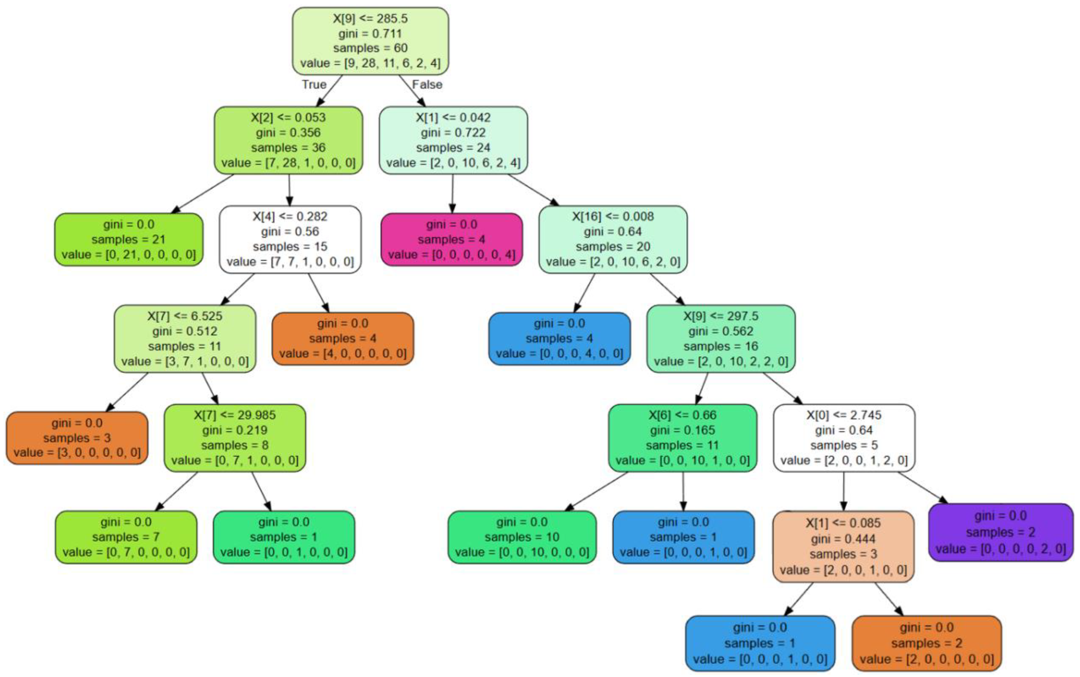
4.3. Decision Tree Analysis

Based on the CART algorithm model, decision tree modeling was performed with the above 20 indicators as independent variables and the PM_2.5 concentration as the dependent variable. The decision tree analysis results are shown in Figure 5. The first line of each node is the name of the attribute used to split the node, i.e., the splitting indicator (X[9] is the land use intensity, X[1] is the comprehensive porosity, X[16] is the ratio of the height to the total floor area, X[2] is the urban canopy resistance, X[4] is the vegetation cover, X[7] is the spatial congestion rate, X[6] is the building density, and X[0] is the average building plot ratio). The second line is the Gini index, which is a measure for assessing the purity. The Gini coefficient reflects the probability that two samples are randomly drawn from the dataset D and the categories are not the same. When using CART decision trees, the Gini index can help us find the best way to split nodes. The lower the Gini index, the more homogeneous the samples contained in the nodes and the higher the purity of the nodes. Therefore, in the construction process of the decision tree, choosing the feature with the smallest Gini index as the criterion for node splitting can make the sub-nodes constructed by the decision tree relatively more pure, which improves the accuracy of the prediction. The label samples denote the number of samples contained in the node. The value indicates how many samples are contained in the different categories, and the one with the largest number of samples is the category of the node. In addition, the different categories of values comprise the six levels of the PM_2.5 concentration (from left to right), namely, the DAQI2, DAQI3, DAQI4, DAQI5, DAQI6, and DAQI7 classes. The decision tree depicted in Figure 5 was organized to obtain the following classification rules (

Table 4. Classification rules for PM_2.5 exposure levels and combinations of dominant morphological factors.

Number	Rules
1	LU ≤ 285.5ΛCF ≤ 0.053 → DAQI3(21)
2	LU ≤ 285.5ΛCF > 0.053ΛVC ≤ 0.282ΛSCD ≤ 6.525% → DAQI2(3)
3	LU ≤ 285.5ΛCF > 0.053ΛVC ≤ 0.282ΛSCD > 6.525%ΛSCD ≤ 29.985% → DAQI3(7)
4	LU ≤ 285.5ΛCF > 0.053ΛVC ≤ 0.282ΛSCD > 29.985% → DAQI4(7)
5	LU ≤ 285.5ΛCF > 0.053ΛVC > 0.282 → DAQI2(4)
6	LU > 285.5ΛPo ≤ 0.042 → DAQI7(4)
7	LU > 285.5ΛPo > 0.042ΛRAHFA ≤ 0.008 → DAQI5(4)
8	LU > 285.5ΛPo > 0.042ΛRAHFA > 0.008ΛLU ≤ 297.5ΛDEB ≤ 0.66 → DAQI4(10)
9	LU > 285.5ΛPo > 0.042ΛRAHFA > 0.008ΛLU ≤ 297.5ΛDEB > 0.66 → DAQI5(1)
10	LU > 285.5ΛPo > 0.042ΛRAHFA > 0.008ΛLU > 297.5ΛAVFAR ≤ 2.745ΛPo ≤ 0.085 → DAQI5(1)
11	LU > 285.5ΛPo > 0.042ΛRAHFA > 0.008ΛLU > 297.5ΛAVFAR ≤ 2.745ΛPo > 0.085 → DAQI2(2)
12	LU > 285.5ΛPo > 0.042ΛRAHFA > 0.008ΛLU > 297.5ΛAVFAR > 2.745 → DAQI6(2)

). The variables in the table are as follows: LU is the land use intensity, CF is the urban canopy resistance, VC is the vegetation cover, SCD is the spatial congestion rate, P_o is the comprehensive porosity, RA_HFA is the ratio of the height to the total floor area, DE_B is the building density, and AV_FAR is the average floor area ratio of buildings.

Table 4 lists the PM_2.5 concentration class distributions and their classification rules among the influencing factors. Among them, Classification rule 1 indicates that when the land use intensity of the neighborhood and block is not higher than 285.5 and the urban canopy resistance is not higher than 0.053, the PM_2.5 concentration varies between 24 and 35 µg/m³, and DAQI3 (21) indicates that 21 samples satisfy the DAQI3 class classification conditions. Rule 2 states that when the land use intensity of the neighborhood and block is not higher than 285.5, the urban canopy resistance is higher than 0.053, the vegetation cover is not higher than 0.282, and the spatial congestion rate is not higher than 6.525%. Similarly, the PM_2.5 concentration in the neighborhood and block ranges from 12 to 23 µg/m³. Rule 3 states that when the land use intensity is not greater than 285.5, the urban canopy resistance is greater than 0.053, the vegetation cover is not greater than 0.282, the spatial congestion rate is greater than 6.525% but less than 29.985%, and the PM_2.5 concentration ranges from 24 to 35 µg/m³. Rule 4 states that when the land use intensity is not higher than 285.5, the urban canopy resistance is higher than 0.053, the vegetation cover is not higher than 0.282, and the spatial congestion rate is higher than 29.985%, the PM_2.5 concentration varies between 36 and 41 µg/m³. Rules 2, 3, and 4 reveal that the spatial congestion rate is closely related to the distribution of the PM_2.5 concentration, i.e., under certain conditions, the higher the spatial congestion rate is, the higher the PM_2.5 concentration. Rule 5 states that when the land use intensity is not higher than 285.5, the urban canopy resistance is higher than 0.053, and the vegetation cover is higher than 0.282, the PM_2.5 concentration ranges from 12 to 23 µg/m³. According to rules 1 and 5, when the urban canopy resistance is greater than the critical value of 0.053, the vegetation cover is the key indicator, i.e., under certain conditions, the higher the vegetation cover is, the lower the PM_2.5 concentration. Rules 2, 3, 4, and 5 indicate that when the vegetation cover is less than the critical value of 0.282, the spatial congestion rate becomes an important judgement indicator. Rule 6 states that when the land use intensity is greater than 285.5 and the comprehensive porosity is not greater than 0.042, the PM_2.5 concentration ranges from 54 to 58 µg/m³. Rule 7 states that when the land use intensity is greater than 285.5, the comprehensive porosity is greater than 0.042, and the height-to-total floor area ratio is not greater than 0.008, the PM_2.5 concentration varies between 42 and 47 µg/m³. Rules 6 and 7 reveal that when the comprehensive porosity is higher than the critical value of 0.042, the ratio of the height to the total floor area becomes a key indicator. As determined by rules 7, 8, and 9, when the land use intensity varies between 285.5 and 297.5 and the ratio of the height to the total floor area is greater than the critical value of 0.008, the building density is directly related to the distribution of the PM_2.5 concentration in the neighborhood and block, i.e., under certain conditions, the PM_2.5 concentration increases with increasing building density. Rules 7 and 12 demonstrate that when the land use intensity is higher than 297.5 and the ratio of the height to the total floor area is higher than the critical value of 0.008, the average floor area ratio of the building becomes an important indicator. According to rules 10 and 11, when the average building volume ratio is not greater than 2.745, the comprehensive porosity exhibits a close relationship with the PM_2.5 concentration, i.e., under certain conditions, the PM_2.5 concentration decreases with increasing comprehensive porosity. Since the PM_2.5 concentration in the built-up areas of Shanghai mainly varies between 20 and 58 µg/m³, the PM_2.5 concentration data of the sample areas were categorized into six levels, i.e., DAQI2 (12–23 µg/m³), DAQI3 (24–35 µg/m³), DAQI4 (36–41 µg/m³), DAQI5 (42–41 µg/m³), DAQI5 (42–47 µg/m³), DAQI6 (48–53 µg/m³), and DAQI7 (54–58 µg/m³). Therefore, DAQI1 was not included in the above decision tree classification rule.

The dominant factors extracted by the decision tree CART algorithm are the land use intensity, urban canopy resistance, vegetation cover, spatial congestion rate, comprehensive porosity, height-to-GFA ratio, building density, and average building volume ratio, covering seven building aspects, including building geometry, ecological landscape distribution, subsurface roughness, street-valley spatial morphology, three-dimensional architectural landscape evaluation, land use and development intensity, and ventilation evaluation index aspects. The feature weighting diagram in Figure 6 shows the importance of these eight indicators to the model. The weight of the land use intensity is 38.58%, the weight of the comprehensive porosity is 13.76%, the weight of the urban canopy resistance is 13.22%, and the weight of the vegetation cover is 10.40%. Moreover, the weights of the ratio of the height to the total floor area, spatial congestion rate, average building volume ratio, and building density are 8.91%, 6.48%, 4.38%, and 4.26%, respectively. Specifically, the weight of the land use intensity is significantly greater than that of the other indicators, indicating that this indicator plays a key role in model construction.

According to the decision tree classification rules (Table 4) and the feature weight diagram (Figure 6), the weight of the land use intensity is significantly higher than that of the other indicators, indicating that it is the most critical indicator. The results of correlation analysis with the PM_2.5 concentration (Table 2) also showed that the land use intensity and PM_2.5 concentration were significantly positively correlated, i.e., within a certain range, the concentration of urban air pollutants increased with increasing land use intensity. The land use intensity is an indicator for evaluating the degree of land use and development. The higher the land use intensity is, the higher the degree of urbanization. An increase in the hard surface area in cities causes the gradual erosion of bare land and land with vegetation cover, increasing the likelihood that air pollutants will stay and accumulate in the air, thus increasing the concentration of air pollutants in cities.

When the land use intensity is greater than the critical value of 285.5, the comprehensive porosity becomes the secondary judgement criterion, and the comprehensive porosity is an index that characterizes the roughness of the urban subsurface. The roughness of the urban subsurface mainly includes the height and unevenness of various man-made and natural objects, such as buildings, roads, squares, and green belts. These uneven surfaces can affect the diffusion and deposition processes of atmospheric pollutants in cities, thus affecting the urban air quality. In addition, the comprehensive porosity is an indicator for evaluating urban spatial ventilation. The higher the porosity of the urban canopy is, the more developed the urban ventilation channels, including street canyons and traffic vessels, thus contributing to air flow and promoting the diffusion and transport of air pollutants.

The third judgement criterion is the urban canopy resistance, which is an indicator of the effectiveness of urban ventilation. A higher urban canopy resistance indicates that city ventilation is poorer, which is not conducive to air pollutant diffusion, and the PM_2.5 concentration is higher.

When the urban canopy resistance is higher than the critical value of 0.053, the vegetation cover becomes the fourth judgement indicator. According to the correlation analysis results in Table 2, the vegetation cover is significantly negatively correlated with the PM_2.5 concentration. Notably, under certain conditions, the higher the vegetation coverage is, the lower the PM_2.5 concentration. This mainly occurs because within a certain area, the higher the vegetation coverage is, the sparser the distribution of buildings, and the obstruction of air flow by the under-cushion surface is reduced, which is conducive to pollutant diffusion [27]. In addition, according to relevant studies [28], plant adsorption plays an important role in reducing atmospheric particulate matter pollution and can effectively improve the air quality.

The fifth criterion is the ratio of the height to the total floor area, which is an indicator of the building geometry. Different building forms exert different effects on pollutant dispersion. This occurs because the building shape affects the surrounding air flow, which in turn affects the dispersion of pollutants.

The sixth criterion is the spatial congestion rate, which usually suggests that the denser the urban space is, the worse the air quality. This occurs because a higher spatial congestion rate at street-level indicates a larger population per unit area, which is associated with more human activities and traffic, and thus more air pollutants. In addition, dense buildings and narrow streets can affect the ventilation conditions, which in turn affects the dispersion of air pollutants. For example, in a poorly ventilated closed space, air pollutants are difficult to remove and thus continuously accumulate, leading to air quality deterioration. However, a well-ventilated open space facilitates pollutant diffusion and dilution and can reduce the concentration of air pollutants.

The seventh criterion is the average building floor area ratio. Similar to the previous analysis, the higher the average building floor area ratio, the more detrimental this is to the air flow, resulting in a large amount of atmospheric particulate matter accumulating in street canyons and contributing to higher PM_2.5 concentrations.

The building density is the last criterion, and the general trend is that the smaller the width of the street canyon, the less conducive this is to pollutant dispersion. This occurs because high-density buildings affect air circulation, resulting in atmospheric pollutants not being effectively diffused, thus creating localized areas of pollution. In addition, dense building complexes increase the traffic flow and population density, which in turn increase pollutant emissions. In terms of meteorological conditions, high-density cities usually experience a significant heat island effect, which can lead to higher temperatures and lower wind speeds in the city, thus affecting pollutant diffusion [29].

According to the final model test results (Figure 7), the final model obtained an accuracy of 86.67% on the test set, a precision (combined) of 87.14%, a recall rate (combined) of 86.67%, and an F1 score (combined) of 0.87, which indicates that the model is suitable to achieve the purpose of this study.

5. Discussion

5.1. Quantification and Thresholds for the Urban Morphological Indicators at Street-Level

According to related research [30], from an architectural perspective, the urban morphology impacts the urban canopy microclimate in two main aspects, namely, the urban street space and the morphology of the urban texture, both of which directly affect the urban canopy resistance and comprehensive porosity. The expression of the urban texture can be divided into two levels: the first level comprises the familiar plot control indicators: building density, building height, building volume, building space congestion rate, and average building volume ratio, which reflect the volume and total capacity of the texture; the second level comprises the building group dispersion [31], neighborhood integration [32], body shape coefficient, and building orientation indicators of the plot buildings, which are indicators of the texture form. These indicators reflect the geometric structural form of the morphology of texture. The combination of these two groups of indicators captures the morphology of the urban fabric. The ratio of the height to the total floor area, building density, spatial congestion rate, and average building volume ratio can be calculated using the values of the building geometry parameters such as the building height, building footprint and volume. The results of the two indicators, i.e., the urban canopy resistance and comprehensive porosity can be obtained according to the street canyon width, and the length, width, height, orientation and bulk coefficients of buildings.

Based on the principle of quantifying the above indicators and combined with statistical analysis and data mining methods, thresholds were obtained for the eight indicators, namely, land use intensity, urban canopy resistance, vegetation cover, spatial congestion rate, comprehensive porosity, height-to-total floor area ratio, building density, and average building volume ratio, which could provide a scientific theoretical basis for street-level refinement planning. Specifically, the land use intensity should not exceed 285.5, the urban canopy resistance should be controlled within 0.053, the vegetation cover should not be less than 28.2%, the spatial congestion rate should be controlled within 6.525%, the comprehensive porosity should not be less than 0.085, the height-to-total floor area ratio should be controlled at approximately 0.008, the building density should be controlled within 66%, and the average building volume ratio should be controlled within 2.745.

5.2. Urban Spatial Optimization Strategies at Street-Level

According to previous studies [33], the layout of urban forms exerts a significant impact on the dispersion and distribution of air pollutants. These effects can be mitigated in three ways: source control, diversion, and convergence [34]. Source control involves controlling pollution by adjusting the land use types and optimizing the layout of road nets. Diversion promotes the diffusion of air pollutants by optimizing the urban morphology and improving the ventilation environment. Convergence promotes the deposition and convergence of particulate matter by utilizing atmospheric particulate matter adsorption and interception by urban green vegetation. Jointly, controlling pollution sources, guiding particulate matter flow and diffusion, and eliminating pollutants and adsorbing pollutants can effectively mitigate air pollution problems in urban districts and promote the development of healthy urban environments. These approaches can be important references for urban planners and policy-makers when formulating urban planning and environmental protection policies.

The preceding paragraph identified eight key combinations of dominant factors (including land use intensity, urban canopy resistance, vegetation cover, spatial congestion rate, integrated porosity, height-to-gross floor area ratio, building density, and average building floor area ratio) that can be considered to improve the ventilation and help control urban air pollution conditions through decision tree analysis. These factors include building geometry, street-valley spatial morphology, subsurface roughness, three-dimensional architectural landscape morphology, ecological landscape distribution, land use and development intensity, and ventilation evaluation indices. In this paper, calculation results for these eight indicators and their thresholds were introduced, and a three-pronged approach involving source control, diversion and convergence was proposed for determining the effect of urban morphology elements on atmospheric particulate matter. A spatial optimization strategy at street-level was developed (

Table 5. Urban optimization strategies at street-level.

Strategies	Spatial Elements	Indicators and Planning Recommendations
Source control	City center	Land use intensity: Control the intensity of construction and development; the intensity should not exceed 285.5.
		Composition: Optimize the layout of land use and the spatial combination pattern of various types of land use, open up important urban ventilation corridors, introduce natural wind into all corners of the districts and neighborhoods, and enhance the ventilation and air exchange capacity.
		Capability: Guide the development of a moderate mix of land functions.
	Roads	Density of the road network: Optimize the road network in the city and appropriately increase the density of the road network, which should not be less than 1%.
		Traffic pattern: Encourage public transportation and green travel.
		Road connectivity: Increase the connectivity between urban roads, reduce the destination detour distance, divert and relieve traffic congestion, improve the traffic efficiency, and realize energy saving and emission reduction.
Diversion	Building	Building density: Control the building density, which should not exceed 66%.
		Average floor area ratio of buildings: avoid high-rise and large-scale buildings and maintain the plot ratio within 2.745.
		Ratio of the height to the total floor area: Control the construction of large-volume single buildings; the ratio of the height to the total floor area should be controlled at approximately 0.008.
		Spatial congestion rate: Appropriate decentralization of buildings and use of differentiated layouts, with a target less than 6.252%.
		Urban canopy resistance: Adopt a small-volume, decentralized building layout and rows and columns of arranged building groups to increase the ventilation gap; control the frontal area ratio by reducing the width and height of buildings along the upwind direction, with the index controlled within 0.053.
	Street canyon	Comprehensive porosity: Appropriately control the height and density of buildings on both sides of the street, optimize the spatial layout of streets, and appropriately increase the width of street canyons; the comprehensive porosity should be greater than 0.085.
Convergence	Green space	Vegetation cover: Appropriately increase green coverage, which should be no less than 28.2%.
		Greenfield connectivity: A large number of wedge-shaped green spaces forming a grid structure should be employed to improve the connectivity between green spaces.
		Green space uniformity: Green spaces should be evenly distributed.

). The whole set of optimization strategies is based on the intrinsic mechanism of the effect of the urban morphology layout on the distribution and diffusion of atmospheric particulate matter, which can provide theoretical references for specific morphology planning and design of green spaces, buildings, streets, etc.

6. Conclusions

Statistical and data mining methods were used to analyze the quantitative relationship between the urban morphological structure and the PM_2.5 concentration. Land use intensity, urban canopy resistance, vegetation cover, spatial congestion rate, integrated porosity, height-to-gross floor area ratio, building density, and average building volume ratio were identified as the key indicators for improving the urban ventilation conditions. These factors are conducive to the control of air pollution and include land use and development intensity, building geometry, street-valley spatial morphology, subsurface roughness, three-dimensional architectural landscape morphology, ecological landscape distribution and ventilation potential. By combining an in-depth examination of the intrinsic mechanism of the influence of the urban morphology on the diffusion and transport of air pollutants with the information mining results for the combinations of dominant morphological factors, a street-level spatial optimization strategy was proposed to improve the urban air quality in terms of source control, diversion and convergence, which could provide a theoretical basis for improving the urban microclimate. Parameters such as air temperature, surface temperature, humidity, wind direction, and wind speed will be introduced in future studies to explore how to integrate urban spatial planning and design with urban ecosystems to enhance the synergy between urban spatial planning and urban ecosystems, so that the whole set of optimization strategies not only offers new dimensions of urban planning and design, but also contributes to the improvement in urban microclimate environments, such as the alleviation of urban heat island effect and air pollution, thereby providing urban residents with liveable and comfortable living environments.

References

1. Aboelata, A. Vegetation in different street orientations of aspect ratio (H/W 1:1) to mitigate UHI and reduce buildings’ energy in arid climate. Build. Environ. 2020, 172, 106712. [Google Scholar] [CrossRef]
2. He, B.-J.; Wang, J.; Liu, H.; Ulpiani, G. Localized synergies between heat waves and urban heat islands: Implications on human thermal comfort and urban heat management. Environ. Res. 2021, 193, 110584. [Google Scholar] [CrossRef]
3. Jadraque Gago, E.; Etxebarria Berrizbeitia, S.; Pacheco Torres, R.; Muneer, T. Effect of Land Use/Cover Changes on Urban Cool Island Phenomenon in Seville, Spain. Energies 2020, 13, 3040. [Google Scholar] [CrossRef]
4. Liao, W.; Liu, X.; Wang, D.; Sheng, Y. The Impact of Energy Consumption on the Surface Urban Heat Island in China’s 32 Major Cities. Remote Sens. 2017, 9, 250. [Google Scholar] [CrossRef]
5. Wang, S.; Zhou, C.; Wang, Z.; Feng, K.; Hubacek, K. The characteristics and drivers of fine particulate matter (PM2.5) distribution in China. J. Clean. Prod. 2017, 142, 1800–1809. [Google Scholar] [CrossRef]
6. Marquez, L.O.; Smith, N.C. A framework for linking urban form and air quality. Environ. Model. Softw. 1999, 14, 541–548. [Google Scholar] [CrossRef]
7. McCarty, J.; Kaza, N. Urban form and air quality in the United States. Landsc. Urban Plan. 2015, 139, 168–179. [Google Scholar] [CrossRef]
8. Han, L. Relationship between urbanization and urban air quality: An insight on fine particulate dynamics in China. Prog. Geogr. 2018, 37, 1011–1021. [Google Scholar]
9. Dai, F.; Chen, M.; Wang, M.; Zhu, S.; Fu, F. Effect of Urban Block Form on Reducing Particulate Matter: A Case Study of Wuhan. Technol. Econ. 2020, 109. [Google Scholar]
10. Long, X.; Bei, N.; Wu, J.; Li, X.; Feng, T.; Xing, L.; Zhao, S.; Cao, J.; Tie, X.; An, Z.; et al. Does afforestation deteriorate haze pollution in Beijing–Tianjin–Hebei (BTH), China? ACP 2018, 18, 10869–10879. [Google Scholar] [CrossRef]
11. Fan, S.; Li, X.; Han, J.; Cao, Y.; Dong, L. Field assessment of the impacts of landscape structure on different-sized atmospheric particles in residential areas of Beijing, China. Atmos. Environ. 2017, 166, 192–203. [Google Scholar] [CrossRef]
12. Yang, J.; Shi, B.; Shi, Y.; Marvin, S.; Zheng, Y.; Xia, G. Air pollution dispersal in high density urban areas: Research on the triadic relation of wind, air pollution, and urban form. Sustain. Cities Soc. 2019, 54, 101941. [Google Scholar] [CrossRef]
13. Yuan, M.; Song, Y.; Huang, Y.; Shen, H.; Li, T. Exploring the association between the built environment and remotely sensed PM2.5 concentrations in urban areas. J. Clean. Prod. 2019, 220, 1014–1023. [Google Scholar] [CrossRef]
14. Luan, Q.; Jiang, W.; Liu, S.; Guo, H. Impact of Urban 3D Morphology on Particulate Matter 2.5 (PM2.5) Concentrations: Case Study of Beijing, China. Chin. Geogr. Sci. 2020, 30, 294–308. [Google Scholar] [CrossRef]
15. Li, S.; Zou, B.; Liu, N.; Feng, H.-H.; Chen, J.; Zhang, H.-H. Simulation of PM2.5 Concentration Based on Optimized Indexes of 2D/3D Urban Form. Environ. Sci. 2022, 43, 4425–4437. [Google Scholar]
16. Cui, P.; Dai, C.; Zhang, J.; Li, T. Assessing the Effects of Urban Morphology Parameters on PM2.5 Distribution in Northeast China Based on Gradient Boosted Regression Trees Method. Sustainability 2022, 14, 2618. [Google Scholar] [CrossRef]
17. Gong, D.; Dai, X.; Zhou, L. Satellite-Based Optimization and Planning of Urban Ventilation Corridors for a Healthy Microclimate Environment. Sustainability 2023, 15, 15653. [Google Scholar] [CrossRef]
18. Edussuriya, P.; Chan, A.; Ye, A. Urban morphology and air quality in dense residential environments in Hong Kong. Part I: District-level analysis. Atmos. Environ. 2011, 45, 4789–4803. [Google Scholar] [CrossRef]
19. Hauke, J.; Kossowski, T. Comparison of Values of Pearson’s and Spearman’s Correlation Coefficients on the Same Sets of Data. Quaest. Geogr. 2011, 30, 87–93. [Google Scholar] [CrossRef]
20. Gao, H. Multivariate-Statistics-Self-Learning; Peking University Press: Beijing, China, 2005. [Google Scholar]
21. Krzywinski, M.; Altman, N. Classification and regression trees. Nat. Methods 2017, 14, 757–758. [Google Scholar] [CrossRef]
22. Hastie, T.; Tibshirani, R.; Friedman, J. Basis expansions and regularization. In The Elements of Statistical Learning; Springer: New York, NY, USA, 2009; pp. 139–189. [Google Scholar]
23. Tian, C.; Cui, Y.; Shen, C.; Chen, X.; Shen, A.; Fan, Q. Estimation of vegetation subsurface Z0 and its improved impact assessment. Environ. Sci. 2022, 42, 3969–3982. [Google Scholar]
24. Watson, D.; Labs, K. Climate Design: Energy Efficient Building Principles and Practices; McGraw-Hill: New York, NY, USA, 1983. [Google Scholar]
25. Huang, Y.; Wu, W.; Fan, B. Numerical simulation of airflow field inside a street canyon with different building aspect ratios. J. Shanghai Univ. Technol. 2005, 3, 203–206. [Google Scholar]
26. Li, S.; Shi, T.; Zhou, S.; Gong, J.; Zhu, L.; Zhou, Y. Diffusion Effects of Atmospheric Pollutants on the Three-Dimensional Landscape Pattern of Urban Block. J. Shenyang Jianzhu Univ. 2016, 32, 1111–1121. [Google Scholar]
27. Ren, C.; Yuan, C.; He, Z.; Wu, E. Research on Urban Ventilation Corridor and Its Planning Application. J. Urban Plan. 2014, 3, 52–60. [Google Scholar]
28. Lyu, L.; Li, H.; Yang, J. The temporal-spatial variation characteristics and influencing factors of absorbing air particulate matters by plants: A review. Chin. J. Ecol. 2016, 35, 524–533. [Google Scholar]
29. Chen, H.; Zhou, X.; Dai, F.; Guan, Y.G. The Study of Urban Ventilation Corridor Planning Based on the Accommodation of Urban Heat Island and Pollutions. Mod. Urban Res. 2014, 7, 24–30. [Google Scholar]
30. Ding, W.; Hu, Y.; Dou, P. A study of the correlation between urban form and urban microclimate. Archit. J. 2012, 7, 16–21. [Google Scholar]
31. Shen, J.; Qiu, X.; He, Y.; Yan, Z.; Li, M. Study on Comparison of Vector/Raster Calculation Model of Frontal Area Density of Urban Buildings. J. Geogr. Inf. Sci. 2017, 19, 1433–1441. [Google Scholar]
32. Ding, W.; Tong, Z. An approach for simulating the street spatial patterns. Build. Simul. 2011, 4, 321–333. [Google Scholar] [CrossRef]
33. Wang, G.; Zhang, W. Effects of Urban Expansion and Changes in Urban Characteristics on PM2.5 Pollution in China. Environ. Sci. 2019, 40, 3447–3456. [Google Scholar]
34. Wang, S.; Yun, Y.; Jia, Q. Ecological Resilience Evaluation of Central Urban Area of Tianjin Based on “Source-Flow-Sink” Index Analysis. J. Hum. Settl. West China 2020, 35, 82–90. [Google Scholar]
Figure 1. Distribution of the 60 sample areas in Shanghai.
Atmosphere 15 00341 g001
Figure 2. Quickbird images of the sample areas with a radius of 200 m for the eight monitoring stations (ah). (a). Changning Xianxia monitoring station (121°23′25″ E, 31°12′21″ N); (b). Jinshan New City monitoring station (121°20′9″ E, 30°44′44″ N); (c). Hongkou monitoring station (121°28′1″ E, 31°18′3″ N); (d). Baoshan Miaohang monitoring station (121°25′54″ E, 31°19′56″ N); (e). Minhang Pujiang monitoring station (121°29′59″ E, 31°4′26″ N); (f). Qingpu Xujing monitoring station (121°17′19″ E, 31°9′59″ N); (g). Pudong New Area monitoring station (121°31′58″ E, 31°13′42″ N); (h). Pudong Zhangjiang monitoring station (121°34′37″ E, 31°12′26″ N).
Atmosphere 15 00341 g002aAtmosphere 15 00341 g002b
Figure 3. PM2.5 concentration field in Shanghai [17].
Atmosphere 15 00341 g003
Figure 4. Wind rose diagram of summer (a) and winter (b) in 2011–2021 in Shanghai.
Atmosphere 15 00341 g004
Figure 5. Decision tree analysis results.
Atmosphere 15 00341 g005
Figure 6. Feature weight map.
Atmosphere 15 00341 g006
Figure 7. Confusion matrix of the test set results.
Atmosphere 15 00341 g007