Predicting Summer Precipitation Anomalies in the Yunnan–Guizhou Plateau Using Spring Sea-Surface Temperature Anomalies

Abstract

By constructing a correlation network between global sea surface temperature anomalies (SSTAs) and summer precipitation anomalies in the Yunnan–Guizhou Plateau, key SST regions influencing summer precipitation anomalies in the Yunnan–Guizhou Plateau were selected. It was found that spring SSTAs in the Bay of Bengal, southwestern Atlantic, and eastern Pacific are crucial for influencing summer precipitation anomalies in the Yunnan–Guizhou Plateau. Setting SSTAs from these three regions as predictor variables 3 months in advance, we constructed multiple linear regression (MLR), ridge regression (RR), and lasso regression (LR) models to predict summer precipitation anomalies over the Yunnan–Guizhou region. The training phase involved data spanning from 1961 to 2005, which aimed to predict precipitation anomalies in the Yunnan–Guizhou Plateau for the period extending from 2006 to 2022. Based on MLR, RR, and LR models, the correlations between predicted values and observed summer precipitation anomalies in Yunnan–Guizhou were 0.48, 0.46, and 0.46, respectively. These values were all higher than the correlation coefficients of the NCC_CSM model’s predicted and observed values. Additionally, its performance in predicting summer precipitation anomalies over the Yunnan–Guizhou region, based on key SST regions, was assessed using performance metrics such as anomaly correlation coefficient (ACC), anomaly sign consistency rate (PC), and trend anomaly comprehensive score (PS score). The average ACC of MLR, RR, and LR models was higher than that of the NCC_CSM model’s predictions. For MLR, RR, LR, and NCC_CSM models, the PCs exceeding 50% of the year were 14, 14, 11, and 10, respectively. Furthermore, the average PS score for predicting summer precipitation anomalies over the Yunnan–Guizhou region using MLR, RR, and LR was approximately 73 points; 8 higher than the average PS score of the NCC_CSM model. Therefore, predicting summer precipitation anomalies over the Yunnan–Guizhou region based on key SST regions is of great significance for improving the prediction skills of precipitation anomalies in this region.

1. Introduction

In meteorological research, understanding the characteristics of precipitation variability is crucial. The precipitation anomalies directly correlate with the occurrence of meteorological disasters such as floods, droughts, and heavy rainfall. The Yunnan–Guizhou Plateau is located in the southwest of China (as shown in Figure 1a). The region is influenced both by the thermal and dynamic processes emanating from the plateau and by the convergence of warm and moist air masses from the Indian Ocean and the Pacific Ocean, giving it unique weather characteristics typical of low-latitude plateaus [1,2]. The Yunnan–Guizhou Plateau region has complex natural conditions with dense areas of mountains and valleys. The region experiences alternating winter and summer monsoons, leading to diverse climate characteristics [3]. The spatial distribution of precipitation in the Yunnan–Guizhou Plateau exhibits significant regional differences, which are closely related to its distinctive topographical and climatic characteristics [4,5]. In this region, precipitation exhibits significant seasonality. The summer season receives the highest rainfall, accounting for approximately 50% of the annual total. This is followed by the autumn season, which receives about 20% to 30% of the annual rainfall. Spring rainfall accounts for around 20% of the annual precipitation, while winter receives the least; comprising only about 5% of the annual total [6]. Additionally, in the southwestern region, the variability of precipitation is greatest in winter and lowest in summer. The differences in precipitation between spring and autumn are relatively small, and this is likely influenced by the sources of atmospheric moisture [7,8]. In the Yunnan–Guizhou region, summer precipitation is influenced by multiple factors, including topography, monsoons, and tropical cyclones, making precipitation forecasting a significant challenge. Therefore, exploring the influencing factors of summer precipitation anomalies in the southwestern region and establishing reliable prediction models hold significant practical importance.

Approximately 70% of Earth’s surface is covered by oceans, playing a vital role in providing heat and moisture to the atmosphere, as well as supplying energy for atmospheric movement, and significantly influencing atmospheric circulation and climate change [9,10,11]. The Yunnan–Guizhou Plateau is located near the tropical oceans of the Bay of Bengal and the South China Sea, where the Indian monsoon and East Asian monsoon bring abundant moisture from the Bay of Bengal, South China Sea, Arabian Sea, and western Pacific, posing challenges to precipitation forecasting in the region [12,13]. Currently, numerous scholars are focused on understanding the connection between sea surface temperature anomalies (SSTA) and precipitation anomalies in the Yunnan–Guizhou Plateau, resulting in a series of meaningful research findings [14,15]. For instance, Jiang et al. (2017) [16] employed the EOF method to analyze the primary modes and causes of summer precipitation anomalies in the Yunnan–Guizhou region. They discovered that the suppression of convection over the Philippine Sea induced anomalous anticyclones over the northwest Pacific and the southern Tibetan Plateau, leading to increased moisture transport to the Yunnan–Guizhou Plateau and resulting in extreme precipitation anomalies in the region. Moreover, the decay and developing phases of the ENSO and the SSTA of the tropical southeastern Indian Ocean had varying impacts on precipitation in the Yunnan–Guizhou Plateau. Ha et al. (2019) [17] found that the weakening of the South Asian monsoon due to warming SST in the northern Indian Ocean resulted in reduced moisture transport from the Bay of Bengal to the Yunnan–Guizhou Plateau, leading to a significant decrease in summer precipitation from 2003 to 2012 compared to 1993–2002. Wen et al. (2022) [18] found that the positive phase of the Western Pacific Oscillation enhanced abnormal low-level cyclones and anticyclones, causing an earlier onset of the rainy season in the Yunnan–Guizhou Plateau. Consequently, SSTAs in regions such as the northern Indian Ocean, western Pacific, and central-eastern Pacific have a significant impact on summer precipitation anomalies in the Yunnan–Guizhou region.

The climate system is one of the intricate, nonlinear dissipative mega-systems [19,20,21]. In the context of global warming, the increasing frequency of extreme events has objectively heightened the difficulty of seasonal climate prediction. Currently, climate predictions primarily rely on statistical and dynamical methods [22]. Statistical methods excel at utilizing extensive historical data and deriving rules from them but are less adept at capturing the nonlinear features within the climate system [23,24]. Dynamical methods, on the other hand, involve mathematical models to simulate and predict various phenomena and processes in the natural world. Given the complexity of the climate system, solving its mathematical equations analytically has proven difficult. Consequently, numerical methods have gradually gained prominence, with climate numerical simulations emerging as a critical approach [25,26,27]. However, the Yunnan–Guizhou Plateau presents complex natural conditions, posing substantial challenges for numerical model forecasts. Thus, it is necessary to study the summer extreme precipitation in Yunnan–Guizhou area from new perspectives and methodologies.

Over the past few decades, complex network methods have emerged as a crucial tool for unraveling intricate relationship structures within the field of climate research. The complex network is applicable for exploring the distant correlation characteristics within the climate system, analyzing its complexity, and forecasting extreme events [28,29]. For instance, Boers et al. (2014) [30] employed network divergence analysis on a directed network to examine the spatiotemporal distribution of extreme precipitation in South America. Their findings revealed that 60% of extreme precipitation in the central Andes could be predicted in advance, with a 90% prediction rate during El Niño periods. Meanwhile, Wolf et al. (2021) [31] utilized a sliding window approach to investigate the spatiotemporal evolution of synchronized networks during heavy precipitation events in East Asian summer monsoons (from April to August). They placed particular focus on changes in the spatial structure of simultaneous heavy precipitation events and explored the strong precipitation band structure of the mei-yu front during different phases of the East Asian summer monsoon. In summary, complex networks, as a crucial tool for handling and understanding nonlinear issues, provide a solid foundation for further research into precipitation.

Machine learning methods enable systems to automatically learn from vast amounts of empirical data and continually enhance their own performance through iterative processes, gradually improving the accuracy of computations and predictions, thereby obtaining more reliable results [32,33]. The development of machine learning has introduced novel approaches to current climate research, and these models have demonstrated promising results in precipitation forecasting. For example, Davenport et al. (2021) [34] applied CNN to analyze atmospheric circulation patterns associated with extreme precipitation events in the central United States. Their approach successfully identified 91% of extreme precipitation events. Li et al. (2021) [35] employed the antecedent SSTA patterns and machine learning methods to develop three models (ASFP-SVR, ASFP-ELM, ASFP-RF) for integrated, probabilistic, and deterministic drought forecasting in regions including Colorado, Danube, Orange, and Pearl River basins. Among these models, ASFP-ELM exhibited the best spatiotemporal capability for predicting drought events. Fan et al. (2022) [36] utilized deep learning autoencoders to identify summer forecast factors in eastern China and constructed regional key factor prediction models based on machine learning methods for precipitation prediction in this region. Compared to mainstream models, their approach improved forecasting results in the South China region by more than 10%. However, research on predicting summer precipitation anomalies in the Yunnan–Guizhou region using machine learning methods is currently limited.

Therefore, the correlation network between SSTA and summer precipitation anomalies in the Yunnan–Guizhou region is constructed. The main seasons affecting summer precipitation in the Yunnan–Guizhou region were selected based on network connectivity. Then, we analyzed the connection between the SST of the seasons and the summer precipitation in the Yunnan–Guizhou region, identified the key SST area that affects the summer precipitation in the Yunnan Guizhou Plateau, and used these SST areas as prediction factors. Then, we conducted summer precipitation prediction experiments for the Yunnan–Guizhou region using various methods, including multiple linear regression (MLR), ridge regression (RR), and lasso regression (LR). The main structure of this paper is as follows: Section 2 introduces the data and methods; Section 3 discusses the key SST regions affecting precipitation in the Yunnan–Guizhou region and predicts the summer precipitation in the Yunnan–Guizhou region based on the indices of these key SST regions; Section 4 summarizes the results.

2. Data and Methods

2.1. Data

In this study, the monthly precipitation data from 141 meteorological stations in the Yunnan–Guizhou Plateau region for the period of 1961–2022 were obtained from the National Climate Center of the China Meteorological Administration. The spatial distribution of these stations is shown in Figure 1a. Additionally, sea surface temperature (SST) data were acquired from NOAA Extended Reconstructed SST V5 (https://psl.noaa.gov/data/gridded/data.noaa.ersst.v5.html), accessed on 1 March 2023. The data had a horizontal resolution of $2^{°}\times 2^{°}$ during 1961–2022. Furthermore, the NCC_CSM model data has evolved from the monthly average data of the National Climate Center of China MODES seasonal model. The model data are initially presented in a grid format. To facilitate the comparison of various datasets, the grid data from this model are interpolated into station data. Subsequently, specific station data from the Yunnan–Guizhou region within the NCC_CSM model are selected for further analysis.

2.2. Methods

For each station (i.e., longitude–latitude grid point), we calculate the monthly precipitation anomalies (actual monthly precipitation value minus the climatological average) for each calendar month. Here, the average monthly precipitation of the Yunnan–Guizhou Plateau from 1981 to 2010 is used to calculate the climate average [37]. The summer precipitation anomaly is then obtained by averaging the precipitation anomalies for the months of June, July, and August (6–8) at each station in the Yunnan–Guizhou region. The calculation method for SSTAs for each grid point was the same. Additionally, the global SST time series was divided into four groups corresponding to the seasons: spring (March to May), summer (June to August), autumn (September to October), and winter (December to February).

2.2.1. Network Construction

This paper mainly constructs a multivariable coupling network based on anomalies in precipitation over the Yunnan–Guizhou region, and on global spring SSTAs. In this network, nodes $i$ and $j$ represent the Yunnan–Guizhou Plateau station locations and global SST grid points, respectively. The study utilized data from the period 1961–2005 (45 years) as the training dataset; that is, the factor modeling phase is selected, and the period 2006–2022 (17 years) is the post-report test stage. The summer precipitation data for the Yunnan–Guizhou region and global spring SST data for each grid point spanning the period from 1961 to 2005 were subjected to a moving window analysis with a one-year step size and a 30-year window size, resulting in the generation of 15 distinct time windows. Pearson correlation coefficients were calculated to quantify the relationship between the Yunnan–Guizhou Plateau node $i$ and the global SST node $j$ for each of these time windows. Subsequently, a correlation network was constructed for each time window. This approach makes it possible to study the main correlation patterns within individual climate fields simultaneously, as well as between climate fields.

To identify the key SST regions influencing precipitation in the Yunnan–Guizhou Plateau, we selected the strongest correlations between SST nodes and Yunnan–Guizhou Plateau precipitation nodes, disregarding associations below a certain threshold. Here, we chose the top 5% of links with the highest correlations (including both positive and negative correlations) in each windowed network, where the p-value for these links was less than 0.05, as determined by significance testing. Consequently, the adjacency matrix for each windowed network is defined as follows:

$$A_{ij}^h=\left\{\begin{array}{c}1, C_{ij}^h\ge {\mathsf{\Delta }}^h\\ 0, C_{ij}^h<{\mathsf{\Delta }}^h\end{array}\right.$$

(1)

where $C_{ij}^h(h=\mathrm{1,2},\cdots 15)$ represents the correlation coefficients between nodes in each windowed network, and ${\mathsf{\Delta }}^h$ represents the correlation threshold within each windowed network. To identify the strength of correlations between specific nodes and other nodes within the network, we employed area-weighted connectivity to characterize the strength of internal associations within the system. For node j, the area-weighted connectivity $S_j$ is defined as follow:

$$S_j=mean\left(\frac{\sum _{ij}{A}_{ij}^h\cos \left({\lambda }_j\right)}{\sum _{ij}\cos \left({\lambda }_j\right)}\right)$$

(2)

where ${\lambda }_j$ represents the latitude of node $j$, and $\cos \left({\lambda }_j\right)$ calculates the weight with respect to the surface area.

2.2.2. Model Prediction Method

This study utilized the period from 1961 to 2005 as the modeling phase and the period from 2006 to 2022 as the verification phase. During the research process, multiple prediction methods were employed, including MLR, RR, and LR models.

(1)

MLR model

The MLR model is used to describe the correlation between a dependent variable and multiple independent variables. The model is represented as:

$$y={\beta }_0+{\beta }_1{X}_1+{\beta }_2{X}_2+\cdots +{\beta }_n{X}_n+\epsilon$$

(3)

where $y$ is the dependent variable, $X_i(i=\mathrm{1,2},\cdots n)$ are the independent variables, ${\beta }_i(i=\mathrm{1,2},\cdots n)$ are unknown parameters, and $\epsilon$ is the random error term [38].

(2)

RR and LR models

RR is an important regression method with advantages such as interpretability and strong generalization. Essentially, it is an improved form of least squares estimation, where a regularization term in the form of an $L_2$ norm is added to the least squares estimation objective function. The objective function for RR is as follows [39]:

$${\widehat{\beta }}_{ridge}=\underset{\beta }{\mathit{arg\; min}}{‖y-X\beta ‖}_2^2+\lambda {‖\beta ‖}_2^2$$

(4)

Here, ${‖y-X\beta ‖}_2^2$ represents the $L_2$-norm loss function, ${‖\beta ‖}_2^2$ is the $L_2$-norm penalty on $\beta$, and $\lambda$ is the tuning parameter. As $\lambda$ increases, the model’s variance gradually decreases while the bias increases. Therefore, finding an appropriate value for $\lambda$ is crucial, and the paper uses cross-validation to determine the value of $\lambda$.

LR is a classical variable selection model that addresses the limitations of least squares and stepwise regression in dealing with multicollinearity, particularly for high-dimensional small-sample data [40,41]. Unlike ridge regression, which cannot eliminate variables, the LR model replaces the $L_2$ norm penalty with an $L_1$ norm penalty, effectively shrinking the regression coefficients of non-significant variables to zero in the LR model. The objective function for LR is as follows [39]:

$${\widehat{\beta }}_{Lasso}=\underset{\beta }{\mathit{arg\; min}}{‖y-X\beta ‖}_2^2+\lambda {‖\beta ‖}_1$$

(5)

Here, $\lambda$ is the coefficient of the penalty term, controlling the model’s complexity.

2.2.3. Methods for Evaluating Predictive Skills

There are numerous methods available for objectively quantifying and evaluating prediction results. In this paper, the primary evaluation methods utilized include anomaly correlation coefficient (ACC), the temporal correlation coefficient (TCC), anomaly sign consistency rate (PC), the pattern similarity (PS) score, and the root mean square error (RMSE). The model evaluation is mostly measured by precipitation anomaly percentage, so it is necessary to calculate the anomaly percentage. The observed value of precipitation anomaly percentage is given by $\left(\left(x_i-\overline{x_i}\right)/\overline{x_i}\right)\times 100\%$, and the predicted value of the Yunnan–Guizhou precipitation model is given by $\left(\left(y_i-\overline{x_i}\right)/\overline{x_i}\right)\times 100\%$, where $x_i$ is the observed value of precipitation anomaly, $y_i$ is the model precipitation anomaly, and $\overline{x_i}$ is the average value of observed precipitation during the climate reference period from 1981 to 2010 [38,42].

ACC assesses spatial similarity, primarily reflecting the degree of similarity between forecasted values and observed values. The calculation formula for ACC is as follows:

$${ACC}_h=\frac{{\sum }_{f=1}^N\left(X_{hf}-\overline{X_f}\right)\times \left(Y_{hf}-\overline{Y_f}\right)}{\sqrt{{\sum }_{f=1}^N{\left(X_{hf}-\overline{X_f}\right)}^2\times \sum _{f=1}^N{\left(Y_{hf}-\overline{Y_f}\right)}^2}}$$

(6)

Here, $N$ represents the total number of prediction results, $X$ is the observed value, $Y$ is the predicted value, $\overline{X_f}$ and $\overline{Y_f}$ represent the spatial average of all observed, and predicted lattice anomaly percentage is the observed value. This evaluation is performed for the entire forecasting domain at a fixed time. ACC falls within the range of −1 to 1. A higher ACC indicates a greater spatial similarity, with ACC = 1 indicating a perfect spatial distribution match.

TCC serves as an effective measure of the statistical capacity of the model to predict anomalies at different grid points. When calculating TCC, it is necessary to first compute the mean squared differences and covariances for each grid point. The formula is as follows:

$${TCC}_f=\frac{{\sum }_{h=1}^M\left(X_{hf}-\overline{X_h}\right)\times \left(Y_{hf}-\overline{Y_h}\right)}{\sqrt{{\sum }_{h=1}^M{\left(X_{hf}-\overline{X_h}\right)}^2}\times \sqrt{{\sum }_{h=1}^M\times {\left(Y_{hf}-\overline{Y_h}\right)}^2}}$$

(7)

Here, $-1\le TCC\le 1$; the larger the TCC, the higher the temporal correlation, indicating a greater consistency in the change trends between observed anomalies and predicted anomalies.

The anomaly sign consistency rate (PC) is an effective method of the China National Climate Center for inspecting the forecast results. It refers to the percentage of stations in which the signs of the predicted values and the actual values’ anomalies are the same. The specific calculation formula is as follows:

$$PC=\frac{N_t}{N}\times 100$$

(8)

Here, $N$ represents the total number of stations. $N_t$ represents the number of meteorological stations in which the signs of predicted value and actual value anomalies are the same.

The trend anomaly comprehensive scoring (PS score), developed by the China National Climate Center, serves as a tool to assess prediction performance. The evaluation formula for prediction performance at each station is as follows [42,43]:

$$PS=\frac{a{N}_0+b{N}_1+c{N}_2}{\left(N-N_0\right)+a{N}_0+b{N}_1+c{N}_2+M}\times 100$$

(9)

Here, $N$ represents the total number of stations, $N_0$ signifies the number of stations with correct trend predictions, $N_1$ denotes the number of stations with correct level-1 anomaly predictions (level-1 anomaly: 20% ≤ precipitation anomaly percentage <50% or −50% ≤ precipitation anomaly percentage < −20%), $N_2$ represents the number of stations with correct level-2 anomaly predictions (level-2 anomaly: precipitation anomaly percentage ≥ 50% or precipitation anomaly percentage ≤ −50%), and $M$ represent the number of level-2 anomalies that were missed. Here, the coefficients $a=2$, $b=2,$ and $c=4$ are weighting factors.

RMSE is a measure of the deviation between observed values and true values. A smaller RMSE indicates better model prediction performance. When RMSE is 0, it means that the forecast results are completely consistent with the actual observation, and it is defined as follows:

$$RMSE=\frac{1}{N}\sum _{i=1}^N{\left(Y_i-X_i\right)}^2$$

(10)

Here, $N$ represents the total number of stations, $Y_i$ represents forecasted values, $X_i$ represents actual observed values.

3. Results

In the summer, there are noticeable year-by-year variations in precipitation on the Yunnan–Guizhou Plateau, with increases or decreases observed in different periods (as shown in Figure 1b). To explore the relationship between global SSTAs in different seasons and summer precipitation anomalies in the Yunnan–Guizhou Plateau, we calculate correlation coefficients between summer precipitation in the Yunnan–Guizhou region and SSTAs in spring, winter, the preceding autumn, and the preceding summer, respectively. The maximum absolute value among these four correlations is taken as the correlation coefficient between the nodes $i$ and the nodes $j$. By retaining the top 5% links, a correlation network is constructed, and the connectivity of this network is calculated. Here, the network connectivity between node $i$ and $j$ corresponds to the correlation of summer precipitation with one of the SSTAs in the four seasons: spring, winter, preceding autumn, or preceding summer. We retain the connectivity which have the maximum correlation value, while assigning a connectivity value of 0 for other seasons. The network connectivity between spring SSTAs and summer precipitation anomalies covers a larger area, which is much stronger than other seasons, indicating that the influence of spring SSTA on summer precipitation anomalies in the Yunnan–Guizhou region is particularly significant. The spatial structure of the network connectivity is similar to Figure 2. Therefore, this study considers the global spring SSTA field (March–May) as the predictor field and Yunnan–Guizhou summer (June–August) precipitation as the predicting field.

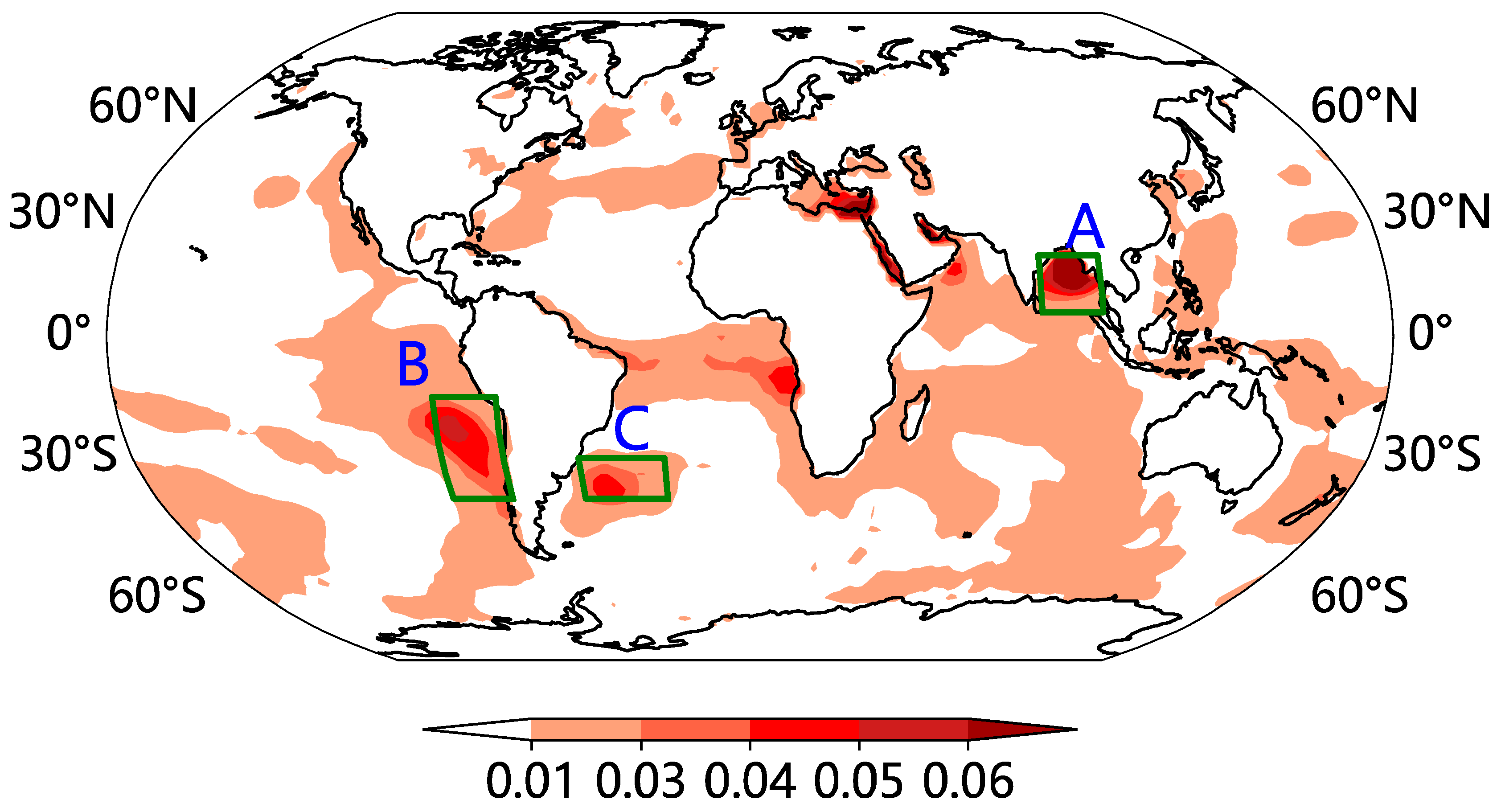
3.1. Selection of Key SSTA Regions

From Figure 2, we observe that the equatorial Indian Ocean, the equatorial south Atlantic, the southwest Atlantic and the east Pacific region have greater connectivity. These regions show a strong correlation with precipitation anomalies in the Yunnan–Guizhou Plateau. In order to verify the robustness of the above results, 25 time windows were obtained by sliding for precipitation anomalies in Yunnan–Guizhou area and global SSTAs with a step size of 1 and a window of 20 years for each grid, and then an unweighted bivariate coupling network was constructed for each window. It was found that the key SSTA zone affecting precipitation on the Yunnan–Guizhou Plateau and the window were the same as those with 30 years (as shown in Figure 2). Therefore, the results of 30 years after using a sliding window are adopted.

SST changes are fundamental drivers of tropical weather systems such as monsoon precipitation and tropical cyclones. The variations in SST within the Bay of Bengal exert a substantial influence on precipitation anomalies in the Yunnan–Guizhou region, serving as a crucial source of atmospheric moisture in this area [44,45]. The eastern Pacific SSTA triggers tropical convective activity, leading to westerly anomalous northward spans. This then alters the east–west circulation of the subtropical Pacific, resulting in east–west asymmetry in the subtropical Indo-Pacific region. These phenomena significantly impact Yunnan–Guizhou precipitation [46]. There is a teleconnection between the SSTAs of the southwestern Atlantic Ocean and the precipitation of the Yunnan–Guizhou Plateau. The SSTAs in the southwestern Atlantic Ocean strongly influence the Yunnan–Guizhou Plateau’s summer precipitation through the Indian summer monsoon, the southwestern monsoon flow, and the South China Sea summer monsoon [36]. Due to the significant impact of SSTAs in the Bay of Bengal, the southwestern Atlantic, and the eastern Pacific on precipitation anomalies in the Yunnan–Guizhou region. Therefore, this study selects the SSTA in the Bay of Bengal, the southwestern Atlantic, and the eastern Pacific as the predictive factors for precipitation on the Yunnan–Guizhou Plateau (corresponding to regions A, B, and C in Figure 2).

For further observation of the relationship between SSTAs in the Bay of Bengal, southwestern Atlantic, and eastern Pacific, and precipitation anomalies in Yunnan–Guizhou, regression analyses were conducted using SST indices from three regions. Here, the average SST in the A (82°−99° E, 6°−20° N), B (80°−90° W, 15°−40° S), and C (25°−50° W, 30°−40° S) regions were used as the SST indices for the Bay of Bengal, eastern Pacific, and southwestern Atlantic, respectively. Through Figure 3, we observe that SSTAs in the Bay of Bengal primarily influence precipitation in the Guizhou region, while SSTA in the southwestern Atlantic and eastern Pacific mainly impact precipitation in Yunnan. Notably, the regression analysis demonstrates that the significance of Bay of Bengal SSTAs against Yunnan–Guizhou precipitation is observed at 28% of the stations. Similarly, the regressions of southwestern Atlantic and eastern Pacific SSTAs against the Yunnan–Guizhou region’s precipitation exhibit significance at 40% and 26% of the stations, respectively.

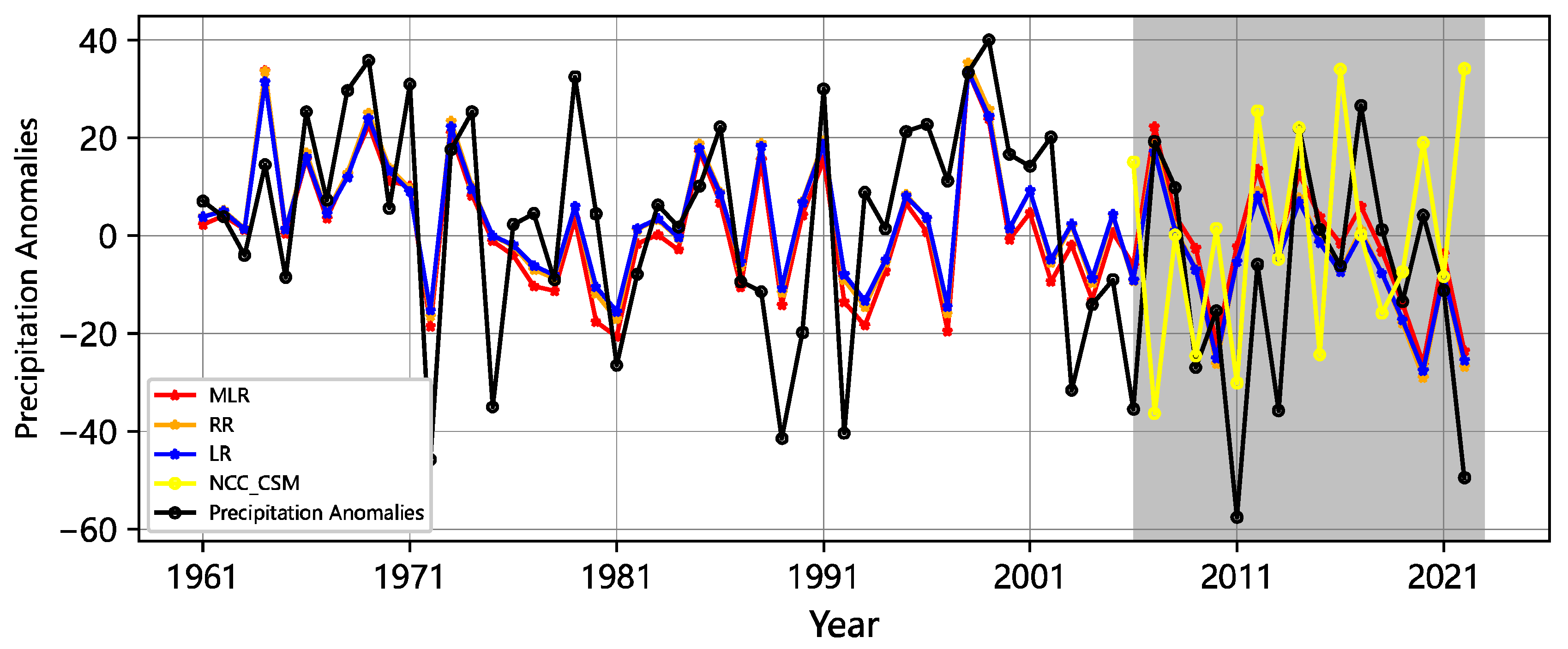
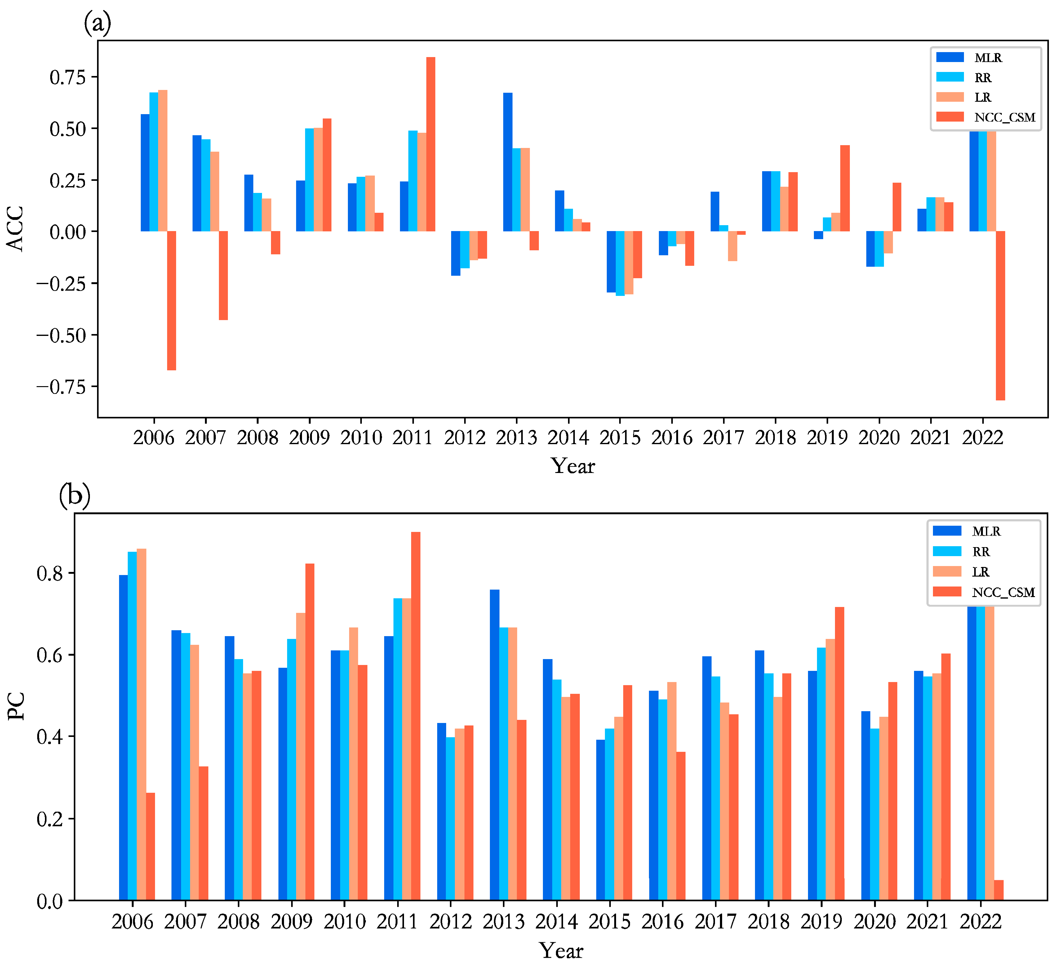
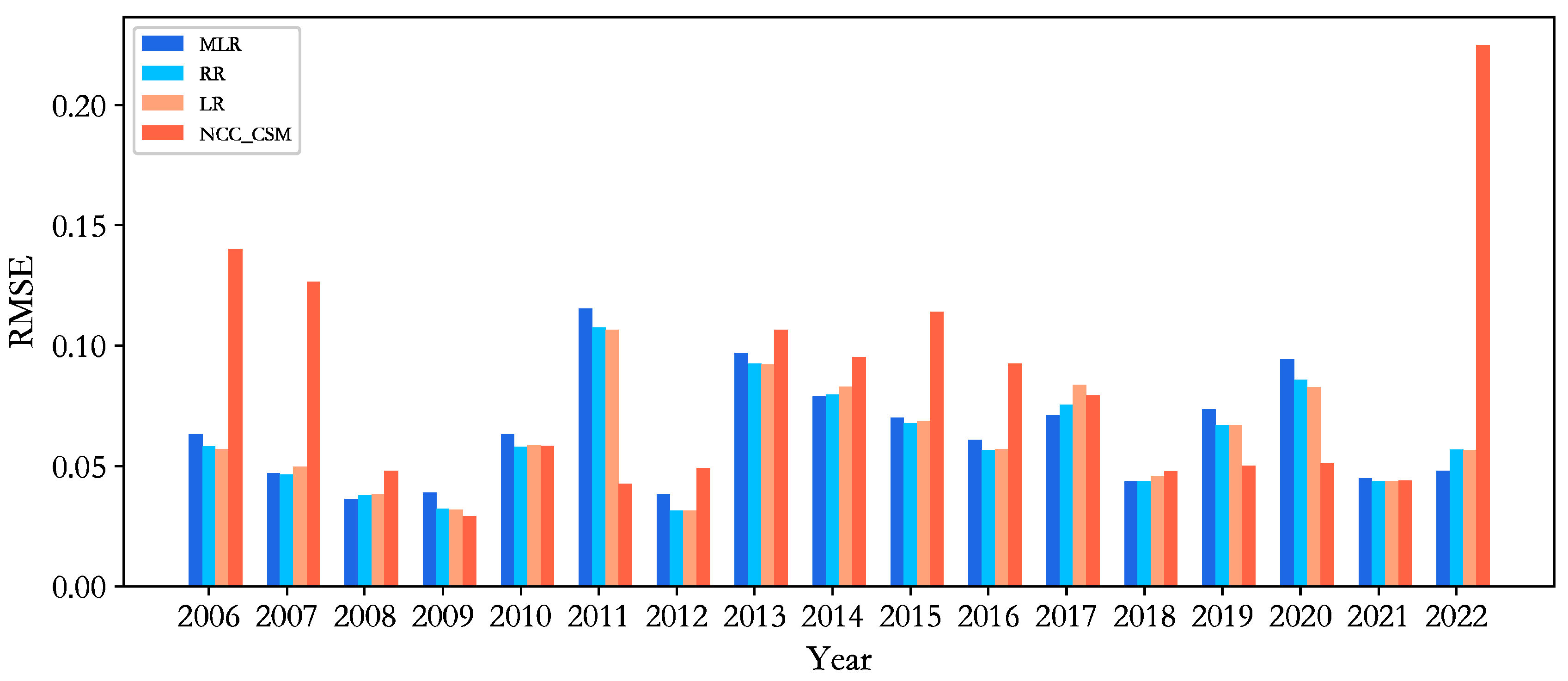
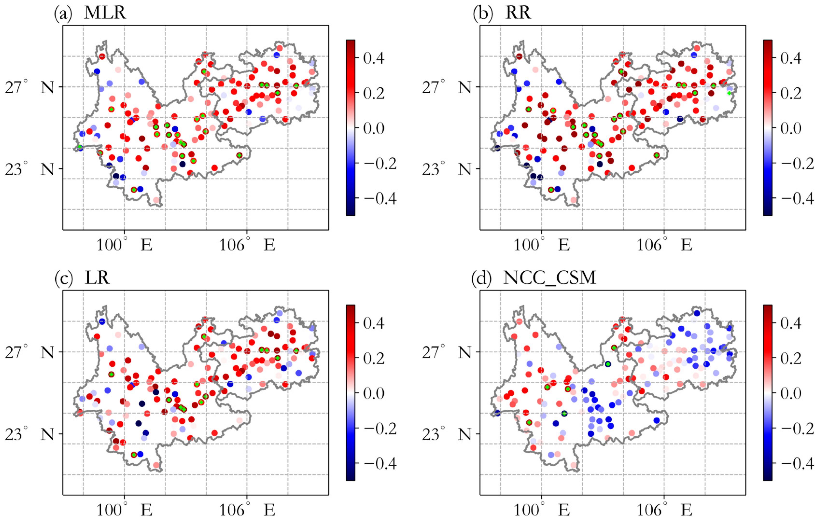
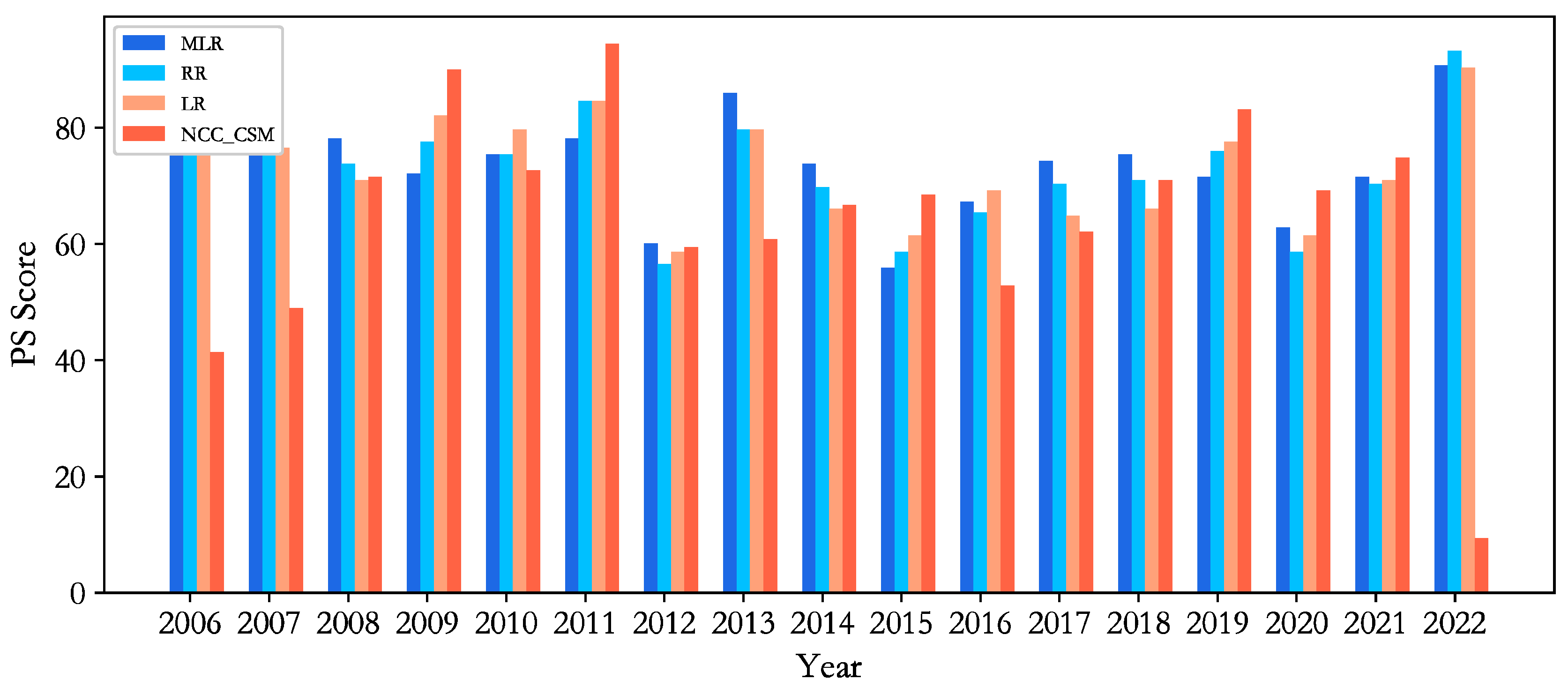
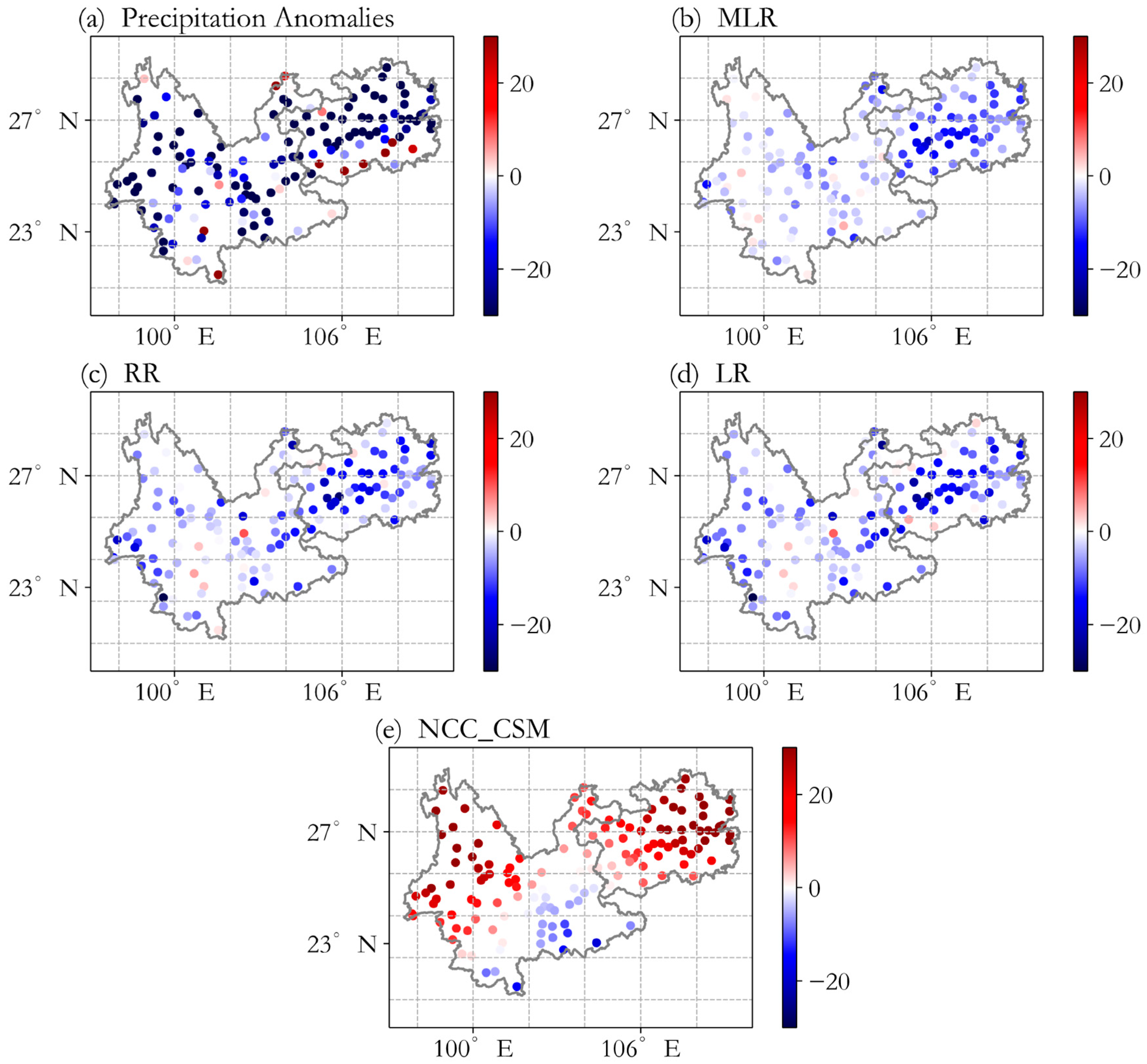
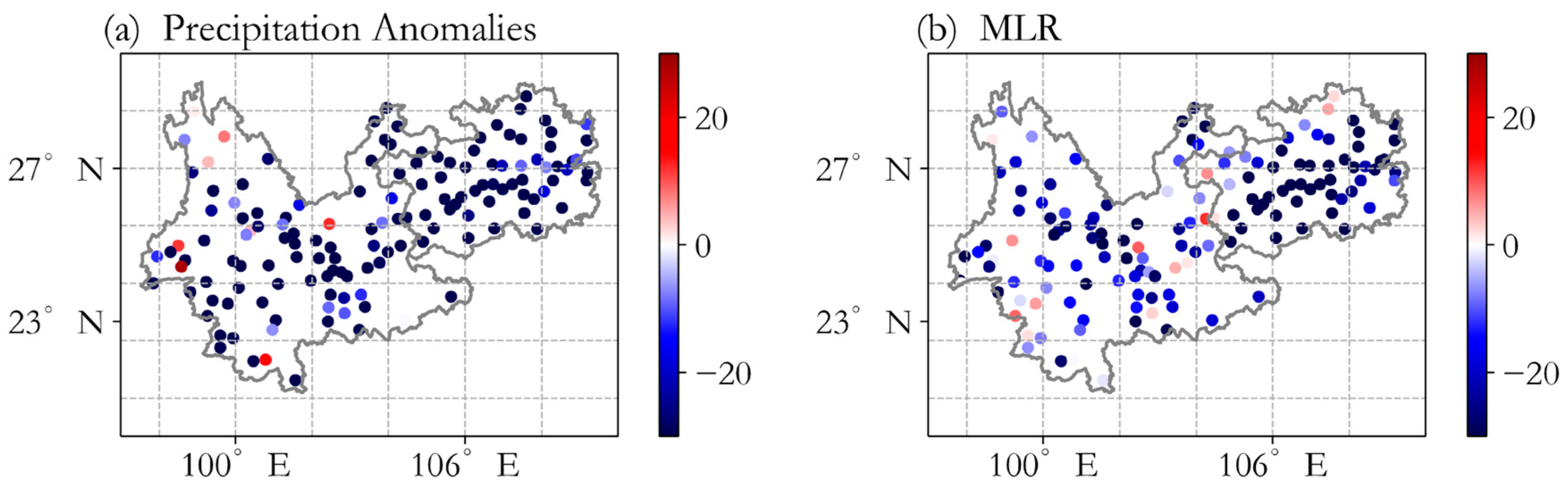
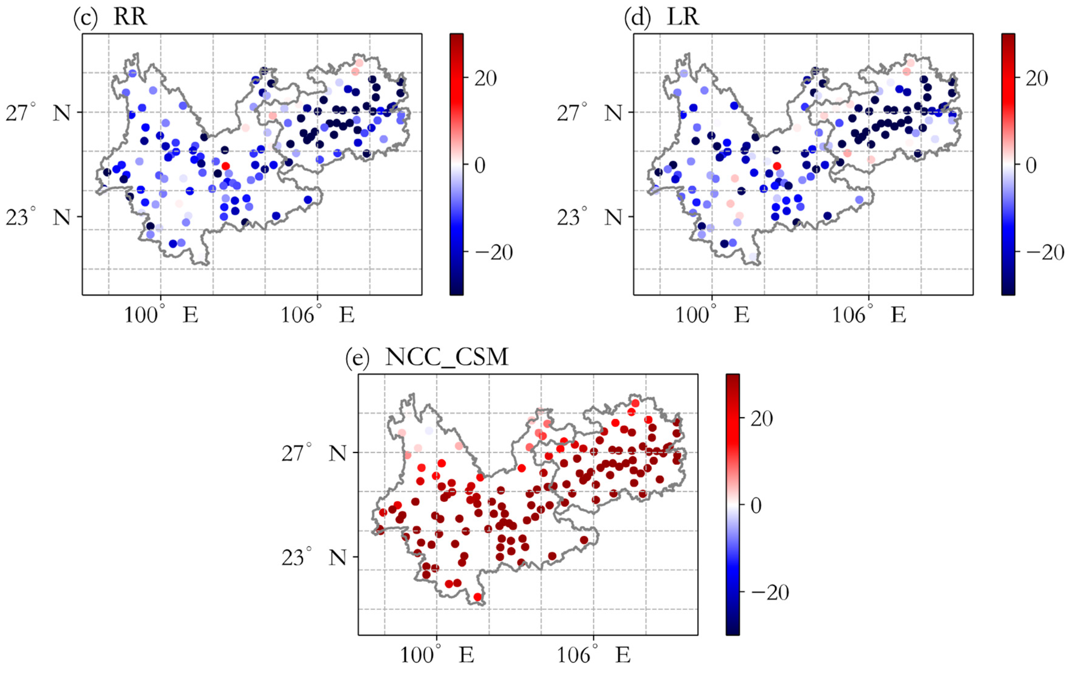
3.2. Prediction Result Analysis

Due to the influence of SSTA in the Bay of Bengal, the southwestern Atlantic, and the eastern Pacific regions on the summer precipitation anomalies in the Yunnan–Guizhou Plateau, this study uses the spring SST indices of these three regions as predictive factors. The model performance during the fitting period of 1961–2005 (training set) is cross-validated in this paper. MLR, RR, and LR are utilized to model precipitation anomalies in the Yunnan–Guizhou region. The aim is to assess the predictive capability of key SST areas for summer precipitation anomalies in the Yunnan–Guizhou Plateau. By employing MLR, the correlation between the fitted results and the observed precipitation anomalies in the Yunnan–Guizhou Plateau during the summer is 0.6. The correlation coefficients based on RR and LR for the predicted precipitation results in the Yunnan–Guizhou region and the observed data are both 0.61 (as shown in Figure 4). The correlations between the predicted precipitation anomalies values and the observed precipitation anomalies in the Yunnan–Guizhou region, using the above three methods, have all passed the significance test at a confidence level of 95% (p < 0.05).

Utilizing data for model fitting from 1961 to 2005, this study forecasts precipitation anomalies in the Yunnan–Guizhou region from 2006 to 2022. According to Figure 4, We found that by employing MLR, RR, and LR, the correlations between the predicted and observed precipitation anomalies in the Yunnan–Guizhou region are 0.48, 0.46, and 0.46, respectively. The correlations between predictions of summer precipitation anomalies in the Yunnan–Guizhou region, made using MLR, RR, and LR methods, and the observed precipitation all surpass the 95% confidence level (p < 0.05). However, it was only in 2007, 2016, and 2021 that the forecasts generated by MLR, RR, and LR closely aligned with the observed values. Additionally, these techniques generally produced lower predictions for summer precipitation anomalies in the Yunnan–Guizhou region and demonstrated weaker performance in predicting extreme precipitation events. On the other hand, the predicted results from the NCC_CSM model of the National Climate Center of China have a correlation coefficient of only −0.003 with the observed results and did not pass the significance test, indicating relatively poor prediction performance. Moreover, for the majority of years, the NCC_CSM model predicts summer precipitation anomalies in the Yunnan–Guizhou region with a sign opposite to that of the actual precipitation anomalies. This indicates that the predictive performance of utilizing the Sea Surface Temperature Anomalies (SSTAs) indices of the Bay of Bengal, east Pacific, and southwest Atlantic for forecasting summer precipitation anomalies exceeds that of the NCC_CSM model.

Here, utilizing MLR, RR, and LR, this study predicts precipitation anomalies at various stations in the Yunnan–Guizhou region based on key sea surface temperature areas. Following that, the model’s effectiveness in predicting precipitation anomalies in the Yunnan–Guizhou region is evaluated using metrics such as ACC, PC, TCC, RMSE, and PS. Among the metrics employed, ACC serves as a widely used measure in climate prediction for assessing the model’s predictive capabilities. In our assessment of the models’ ability to predict abnormal precipitation in the Yunnan–Guizhou region, we compare the ACC of various models; encompassing MLR, RR, LR, and the NCC_CSM model. As shown in Figure 5a, the ACC for predicting summer precipitation anomalies in the Yunnan–Guizhou region based on MLR was negative only in the years 2012, 2015, 2016, 2019, and 2020. The ACC for predicting the same using RR was negative only in 2012, 2015, 2016, and 2020, with positive values in other years. The results for LR in predicting summer precipitation anomalies in the Yunnan–Guizhou region are similar to those of MLR and RR. However, in some years, especially 2012, 2015, 2016, and 2020, there is lower similarity or even an opposite pattern in precipitation distribution. On the other hand, the ACC for the NCC_CSM mode surpasses that derived from spring key SST for predicting summer precipitation in the Yunnan–Guizhou region only in the years 2009, 2011, 2019, and 2020. In general, the ACC for forecasting summer precipitation anomalies in the Yunnan–Guizhou region, based on key SST areas, is higher than that of the NCC_CSM model.

The PC is also a commonly employed method to evaluate the effectiveness of model predictions, as it can only capture the primary trend in precipitation forecasts when the PC exceeds 50%. Observing Figure 5b, in the prediction of summer precipitation anomalies in the Yunnan–Guizhou region from 2006 to 2022 using the MLR and RR methods, there are 14 years in which the PC exceeded 50%. The LR method has the fewest years in which PC exceeded 50%, with only 11 years. However, the NCC_CSM model has a PC exceeding 50% in only 10 years, from 2006 to 2022. Next, we observe the RMSE of precipitation anomaly predictions for the Yunnan–Guizhou region from 2006 to 2022 based on MLR, RR, LR, and the NCC_CSM model, as shown in Figure 6. We found that for 9 of the observed years, the RMSE of the NCC_CSM model is higher than that of MLR, RR, and LR. Only in the years 2009 and 2019, was the RMSE of the NCC_CSM model lower than that of MLR, RR, and LR models. This indicates that the predictive performance of the MLR, RR, and LR models is relatively good.

The time correlation coefficient of the Yunnan–Guizhou precipitation forecast based on MLR, RR, LR, and NCC_CSM model was observed in Figure 7. The TCC test evaluates the forecasting ability of each station, where a higher TCC indicates higher prediction skill, and vice versa. From the TCC distribution, it can be shown that the NCC_CSM model has significantly fewer sites passing the significance test, accounting for only 4% of the total sites, and indicating a relatively lower predictive capability. In contrast, the TCC for predicting summer precipitation anomalies in the Yunnan–Guizhou region based on MLR has the highest number of sites passing the significance test, at 16%. Following closely is the TCC for RR, with 14% of the sites passing the significance test. The TCC for summer precipitation anomalies prediction in the Yunnan–Guizhou region based on LR has the lowest percentage of sites passing the significance test, standing at 9%; although this is still higher than that of the NCC_CSM model.

In order to further test the prediction effect of the model on the precipitation anomalies in the Yunnan–Guizhou region, the PS score was used to test the prediction of the precipitation anomaly in the Yunnan–Guizhou Plateau. Based on MLR, RR, and LR, the average PS scores for predicting summer precipitation anomalies in the Yunnan–Guizhou region are all around 73, as shown in Figure 8. Specifically, when predicting summer precipitation anomalies in the Yunnan–Guizhou region from 2006 to 2022 using MLR, the PS scores exceeded 70 in 13 years and surpassed 80 in 2006, 2013, and 2022. For RR, predicting summer precipitation in the Yunnan–Guizhou region from 2006 to 2022 resulted in PS scores exceeding 70 in 12 years. In the case of LR, 10 years saw PS scores surpassing 70. On the other hand, the average PS score for predicting summer precipitation anomalies in the Yunnan–Guizhou region based on the NCC_CSM model is only 65, with scores exceeding 70 in only 7 years. The above analysis demonstrates the effective prediction of summer precipitation trends on the Yunnan–Guizhou Plateau using SSTA in three distinct regions: the Bay of Bengal, the southwestern Atlantic, and the eastern Pacific. This information serves as a valuable reference for anticipating precipitation anomalies on the Yunnan–Guizhou Plateau.

To gain a more intuitive understanding of predicting precipitation anomalies on the Yunnan–Guizhou Plateau using spring SSTA, we selected 2 years with high ACC in forecasting summer precipitation in the Yunnan–Guizhou region based on key SST regions. we compared predicted and observed precipitation anomalies from 2006 and 2022. This allowed us to observe the effectiveness of precipitation predictions over the past two years. Through Figure 9, we compare the anomaly values predicted by MLR, RR, LR, and the NCC_CSM model with the observed anomaly values. We observed that, based on MLR, RR, and LR, the precipitation anomaly predictions for the central part of Guizhou in 2006 were relatively accurate on the Yunnan–Guizhou Plateau. In contrast, the predicted values for the Yunnan region were relatively smaller compared to the observed values. However, the NCC_CSM model predictions closely align with observed values only in the southern part of Yunnan, with predictions and observations anomalies exhibiting almost entirely opposite patterns in other regions. This might be attributed to the intricate terrain of the Yunnan–Guizhou region, posing challenges in forecasting precipitation anomalies in the area. Examining the observed and predicted precipitation anomalies in the Yunnan–Guizhou region for the year 2022 through Figure 10, it is evident that the NCC_CSM model predicts exclusively positive values for the Yunnan–Guizhou region. However, the observed precipitation anomalies in the Yunnan–Guizhou region exhibit mostly negative values across most grid points, revealing a contrasting pattern between the predicted and observed precipitation anomaly values in the majority of grid points. In contrast, MLR, RR, and LR exhibited better predictions for the Yunnan–Guizhou region, where the majority of points displayed consistent signs of precipitation anomaly between predictions and observations. Among them, the predicted and observed values in the central part of Guizhou are the closest. However, in the Yunnan region, the predicted values from MLR, RR, and LR are relatively lower. In general, for most sites in 2006 and 2022, MLR, RR, and LR exhibited consistent signs of precipitation anomalies compared to observations. Furthermore, forecasting summer precipitation in the Yunnan–Guizhou region based on the Bay of Bengal, east Pacific, and southwest Atlantic exhibits more advantages compared to the NCC_CSM model.

4. Summary and Discussion

This study employs complex network methods to construct a correlation network between SSTA and summer precipitation anomalies in the Yunnan–Guizhou region. It is found that the springtime SSTA in the Bay of Bengal, the southwestern Atlantic, and the eastern Pacific exhibits strong connectivity with the summer precipitation anomalies in the Yunnan–Guizhou region. Therefore, the SSTA in the Bay of Bengal, the southwestern Atlantic, and the eastern Pacific were chosen as predictive variables. MLR, RR, and LR techniques were employed to predict precipitation anomalies in the Yunnan–Guizhou region. Utilizing the training set comprising data from 1961 to 2005, simulations of precipitation anomalies in the Yunnan–Guizhou region were conducted through MLR, RR, and LR. The correlation coefficients between the results obtained from these three methods and the observed summer precipitation anomalies in Yunnan–Guizhou were 0.6, 0.61, and 0.61, respectively. Using the model fitted with data from 1961 to 2005, predictions were generated for precipitation anomalies in the Yunnan–Guizhou region spanning from 2006 to 2022. The correlation between the predicted results and observed data reached 46%, and both passed the 95% confidence level. In contrast, the correlation coefficient between the predictions from the China National Climate Center NCC_CSM model and the observed results was only −0.003, which failed to pass the significance test.

Then, to assess the effectiveness of the predicting summer precipitation anomalies in the Yunnan–Guizhou region based on spring SST, we employed ACC, PC, RMSE, TCC, and PS scores for evaluation. The mean ACC values for the MLR, RR, and LR model predictions were consistently higher than the mean ACC value for the NCC_CSM model. Using MLR, RR, and LR methods for predicting summer precipitation anomalies in the Yunnan–Guizhou region from 2006 to 2022, there were 14, 14, and 11 years, respectively, with PC values exceeding 50%. In contrast, the NCC_CSM model had PC values exceeding 50% for only 10 years. Furthermore, the NCC_CSM model exhibited lower RMSE only in 2009 and 2019 compared to MLR, RR, and LR. In most years, the RMSE of MLR, RR, and LR models was lower than that of the NCC_CSM model. Moreover, utilizing MLR, RR, and LR, the average PS scores for forecasting summer precipitation anomalies in the Yunnan–Guizhou region hover around 73, surpassing the NCC_CSM model’s average PS score of 8 for the corresponding predictions. These results collectively indicate that the predictive performance of MLR, RR, and LR models is relatively superior. Overall, the predictions from the models based on crucial SST regions outperform the simulation results of the NCC_CSM model for summer precipitation in the Yunnan–Guizhou Plateau, enhancing predictive capabilities to some extent. However, limitations exist, including an overall underestimation in predictions and the need for improvement in predicting extreme values.

References

1. Jiang, M.; Lin, Y.; Chan, T.O.; Yao, Y.J.; Zheng, G.; Luo, S.Z.; Zhang, L.; Liu, D.P. Geologic factors leadingly drawing the macroecological pattern of rocky desertification in southwest China. Sci. Rep. 2020, 10, 1440. [Google Scholar] [CrossRef]
2. Wang, S.; Fu, Z.Y.; Chen, H.S.; Nie, Y.P.; Xu, Q.X. Mechanisms of surface and subsurface runoff generation in subtropical soil-epikarst systems: Implications of rainfall simulation experiments on karst slope. J. Hydrol. 2020, 580, 124370. [Google Scholar] [CrossRef]
3. Yang, R.W.; Zhang, W.K.; Gui, S.; Tao, Y.; Cao, J. Rainy season precipitation variation in the Mekong River basin and its relationship to the Indian and East Asian summer monsoons. Clim. Dyn. 2019, 529, 5691–5708. [Google Scholar] [CrossRef]
4. Zhou, L.L.; Xu, G.R.; Xiao, Y.J.; Wan, R.; Wang, J.X.; Leng, L. Vertical structures of abrupt heavy rainfall events over southwest China with complex topography detected by dual-frequency precipitation radar of global precipitation measurement satellite. Int. J. Climatol. 2022, 42, 7628–7647. [Google Scholar] [CrossRef]
5. Qin, N.X.; Chen, X.; Fu, G.B.; Zhai, J.Q.; Xue, X.W. Precipitation and temperature trends for the Southwest China: 1960–2007. Hydrol. Process. 2010, 24, 3733–3744. [Google Scholar] [CrossRef]
6. Shi, P.; Wu, M.; Qu, S.M.; Jiang, P.; Qiao, X.Y.; Chen, X.; Zhou, M.; Zhang, Z.C. Spatial Distribution and Temporal Trends in Precipitation Concentration Indices for the Southwest China. Water Resour. Manag. 2015, 29, 3941–3955. [Google Scholar] [CrossRef]
7. Nie, Y.B.; Sun, J.Q. Causes of Interannual Variability of Summer Precipitation Intraseasonal Oscillation Intensity over Southwest China. J. Clim. 2022, 35, 3705–3723. [Google Scholar] [CrossRef]
8. Lu, C.H.; Huang, D.G.; Chen, B.; Bai, Y.Y. Causes of the Interannual Variation of Summer Precipitation in Eastern Southwest China. Atmosphere 2023, 14, 1230. [Google Scholar] [CrossRef]
9. Duan, W.S.; Song, L.Y.; Li, Y.; Mao, J.Y. Modulation of PDO on the predictability of the interannual variability of early summer rainfall over south China. J. Geophys. Res. Atmos. 2013, 118, 13008–13021. [Google Scholar] [CrossRef]
10. Song, L.Y.; Duan, W.S.; Li, Y.; Mao, J.Y. A timescale decomposed threshold regression downscaling approach to forecasting South China early summer rainfall. Adv. Atmos. Sci. 2016, 33, 1071–1084. [Google Scholar] [CrossRef]
11. Jin, Y.S.; Liu, Z.Y.; Duan, W.S. The Different Relationships between the ENSO Spring Persistence Barrier and Predictability Barrier. J. Clim. 2022, 35, 6207–6218. [Google Scholar] [CrossRef]
12. Li, B.S.; Ding, R.Q.; Qin, J.H.; Zhou, L.; Hu, S.; Li, J.P. Interdecadal changes in potential predictability of the summer monsoon in East Asia and South Asia. Atmos. Sci. Lett. 2019, 20, e890. [Google Scholar] [CrossRef]
13. Zhang, C. Moisture sources for precipitation in Southwest China in summer and the changes during the extreme droughts of 2006 and 2011. J. Hydrol. 2020, 591, 125333. [Google Scholar] [CrossRef]
14. Gong, Z.Q.; Feng, G.L.; Dogar, M.M.; Huang, G. The possible physical mechanism for the EAP-SR co-action. Clim. Dyn. 2018, 51, 1499–1516. [Google Scholar] [CrossRef]
15. Qiao, P.J.; Liu, W.Q.; Zhang, Y.W.; Gong, Z.Q. Complex Networks Reveal Teleconnections between the Global SST and Rainfall in Southwest China. Atmosphere 2021, 12, 101. [Google Scholar] [CrossRef]
16. Jiang, X.W.; Shu, J.C.; Wang, X.; Huang, X.M.; Wu, Q. The roles of convection over the Western Maritime Continent and the Philippine Sea in interannual variability of summer rainfall over Southwest China. J. Hydrometeorol. 2017, 18, 2043–2056. [Google Scholar] [CrossRef]
17. Ha, Y.; Zhong, Z.; Hu, Y.J.; Zhu, Y.M.; Zang, Z.L.; Zhang, Y.; Yao, Y.; Sun, Y. Differences between decadal decreases of boreal summer rainfall in southeastern and southwestern China in the early 2000s. Clim. Dyn. 2019, 52, 3533–3552. [Google Scholar] [CrossRef]
18. Wen, D.Y.; Zhang, J.W.; Cao, J. Impact of the Asian-Pacific Oscillation on the interannual variability of rainy season onset date in Southwest China. Clim. Dyn. 2022, 59, 701–713. [Google Scholar] [CrossRef]
19. Li, J.P.; Chou, J.F. Advances in Nonlinear Atmospheric Dynamics. Chin. J. Atmos. Sci. 2003, 27, 653–673. (In Chinese) [Google Scholar]
20. Fu, Z.T.; Li, Q.L.; Yuan, N.M.; Yao, Z.H. Multi-scale entropy analysis of vertical wind variation series in atmospheric boundary-layer. Commun. Nonlinear Sci. Numer. Simul. 2014, 19, 83–91. [Google Scholar] [CrossRef]
21. He, W.P.; Xie, X.Q.; Mei, Y.; Wan, S.Q.; Zhao, S.S. Decreasing predictability as a precursor indicator for abrupt climate change. Clim. Dyn. 2021, 56, 3899–3908. [Google Scholar] [CrossRef]
22. Gong, Z.Q.; Hutin, C.; Feng, G.L. Methods for Improving the Prediction Skill of Summer Precipitation over East Asia-West Pacific. Weather Forecast. 2016, 31, 1381–1392. [Google Scholar] [CrossRef]
23. Yu, Z.P.; Chu, P.; Schroeder, T. Predictive Skills of Seasonal to Annual Rainfall Variations in the U.S. Affiliated Pacific Islands: Canonical Correlation Analysis and Multivariate Principal Component Regression Approaches. J. Clim. 1997, 12, 2586–2599. [Google Scholar] [CrossRef]
24. Cao, J.; Zhang, W.K.; Tao, Y. Thermal Configuration of the Bay of Bengal-Tibetan Plateau Region and the May Precipitation Anomaly in Yunnan. J. Clim. 2017, 30, 9303–9319. [Google Scholar] [CrossRef]
25. Gong, Z.Q.; Dogar, M.M.; Qiao, S.B.; Hu, P.; Feng, G.L. Assessment and correction of BCC_CSM’s performance in capturing leading modes of summer precipitation over North Asia. Int. J. Climatol. 2017, 38, 2202–2214. [Google Scholar] [CrossRef]
26. Ding, R.Q.; Tseng, Y.H.; Di Lorenzo, E.; Shi, L.; Li, J.P.; Yu, J.Y.; Wang, C.Z.; Sun, C.; Luo, J.J.; Ha, K.J.; et al. Multi-year El Niño events tied to the North Pacific Oscillation. Nat. Commun. 2022, 13, 3871. [Google Scholar] [CrossRef]
27. Duan, W.S.; Feng, R.; Yang, L.C.; Jiang, L. A new approach to data assimilation for numerical weather forecasting and climate prediction. J. Appl. Anal. Comput. 2022, 12, 1007–1021. [Google Scholar] [CrossRef]
28. Tsonis, A.A.; Roebber, P.J. The architecture of the climate network. Physica A 2004, 333, 497–504. [Google Scholar] [CrossRef]
29. Zhang, Y.W.; Fan, J.F.; Li, X.T.; Liu, W.Q.; Chen, X.S. Evolution mechanism of principal modes in climate dynamics. New J. Phys. 2020, 22, 093077. [Google Scholar] [CrossRef]
30. Boers, N.; Bookhagen, B.; Barbosa, H.M.J.; Marwan, N.; Kurths, J.; Marengo, J.A. Prediction of extreme floods in the eastern Central Andes based on a complex networks approach. Nat. Commun. 2014, 5, 5199. [Google Scholar] [CrossRef]
31. Wolf, F.; Ozturk, U.; Cheung, K.; Donner, R.V. Spatiotemporal patterns of synchronous heavy rainfall events in East Asia during the Baiu season. Earth Syst. Dyn. 2021, 12, 295–312. [Google Scholar] [CrossRef]
32. Ling, F.H.; Luo, J.J.; Li, Y.; Tang, T.; Bai, L.; Ouyang, W.L.; Yamagata, T. Multi-task machine learning improves multi-seasonal prediction of the Indian Ocean Dipole. Nat. Commun. 2022, 13, 7681. [Google Scholar] [CrossRef]
33. Chen, G.X.; Wang, W.C. Short-Term Precipitation Prediction for Contiguous United States Using Deep Learning. Geophys. Res. Lett. 2022, 49, e2022GL097904. [Google Scholar] [CrossRef]
34. Davenport, F.V.; Diffenbaugh, N.S. Using Machine Learning to Analyze Physical Causes of Climate Change: A Case Study of U.S. Midwest Extreme Precipitation. Geophys. Res. Lett. 2021, 48, e2021GL093787. [Google Scholar] [CrossRef]
35. Li, J.; Wang, Z.L.; Wu, X.S.; Xu, C.Y.; Guo, S.L.; Chen, X.H.; Zhang, Z.X. Robust Meteorological Drought Prediction Using Antecedent SST Fluctuations and Machine Learning. Water Resour. Res. 2021, 57, e2020WR029413. [Google Scholar] [CrossRef]
36. Fan, J.F.; Meng, J.; Ludescher, J.; Li, Z.Y.; Surovyatkina, E.; Chen, X.S.; Kurths, J.; Schellnhuber, H.J. Network-Based Approach and Climate Change Benefits for Forecasting the Amount of Indian Monsoon Rainfall. J. Clim. 2022, 35, 1009–1020. [Google Scholar]
37. CMA Climate Change Centre. Blue Book on Climate Change in China (2022); Science Press: Beijing, China, 2022. [Google Scholar]
38. Pang, Y.S.; Zhou, B.; Zhu, C.W.; Qin, N.S.; Yang, Y. Multifactor Descending Dimension Method of Objective Forecast for Summer Precipitation in Southwest China. Chin. J. Atmos. Sci. 2021, 45, 471–486. (In Chinese) [Google Scholar]
39. Peña, M.; Vázquez-Patiño, A.; Zhiña, D.; Montenegro, M.; Avilés, A. Improved Rainfall Prediction through Nonlinear Autoregressive Network with Exogenous Variables: A Case Study in Andes High Mountain Region. Adv. Meteorol. 2020, 2020, 1828319. [Google Scholar] [CrossRef]
40. Tibshirani, R. Regression shrinkage and selection via the LASSO. J. R. Stat. Soc. Ser. B Methodol. 1996, 58, 267–288. [Google Scholar] [CrossRef]
41. Bai, H.M.; Gong, Z.Q.; Sun, G.Q.; Li, L. Data-Driven Artificial Intelligence Model of Meteorological Elements Influence on Vegetation Coverage in North China. Remote Sens. 2022, 14, 1307. [Google Scholar] [CrossRef]
42. Zheng, R.; Liu, J.H.M.; Ma, Z.F. Application of an interannual increment method for summer precipitation forecast in Southwest China. Acta Meteorol. Sin. 2019, 77, 489–496. [Google Scholar]
43. Li, T.; Qiao, C.W.; Wang, L.A.; Chen, J.; Ren, Y.J. An Algorithm for Precipitation Correction in Flood Season Based on Dendritic Neural Network. Front. Plant Sci. 2022, 13, 862558. [Google Scholar] [CrossRef] [PubMed]
44. Li, Y.H.; Lu, C.H.; Xu, H.M.; Cheng, B.Y. Anomalies of sea surface temperature in Pacific-Indian Ocean and effects on drought/flood in summer over eastern of Southwest China. J. Trop. Meteorol. 2012, 28, 145–156. [Google Scholar]
45. Qiao, P.J.; Gong, Z.Q.; Liu, W.Q.; Zhang, Y.W.; Feng, G.L.; Dong, W.J. Extreme rainfall synchronization network between Southwest China and Asia-Pacific region. Clim. Dyn. 2021, 57, 3207–3221. [Google Scholar] [CrossRef]
46. Mujumdar, M.; Sooraj, K.P.; Krishnan, R.; Preethi, B.; Joshi, M.K.; Varikoden, H.; Singh, B.B.; Rajeevan, M. Anomalous convective activity over sub-tropical east Pacific during 2015 and associated boreal summer monsoon teleconnections. Clim. Dyn. 2017, 48, 4081–4091. [Google Scholar] [CrossRef]
Figure 1. (a) A map of China and spatial distribution of meteorological observation stations in the Yunnan–Guizhou Plateau. (b) Summer precipitation anomalies in the Yunnan–Guizhou Plateau from 1961 to 2022.
Atmosphere 15 00453 g001
Figure 2. The spatial distribution of connectivity in the correlation network between global spring SSTAs and Yunnan–Guizhou Plateau summer precipitation anomalies. A, B, and C represent the Bay of Bengal, the eastern Pacific, and the southwestern Atlantic, respectively.
Atmosphere 15 00453 g002
Figure 3. The spatial distribution of regression coefficients between SSTA in the (a) Bay of Bengal, (b) eastern Pacific, and (c) southwestern Atlantic regions, and anomalies in summer precipitation over the Yunnan–Guizhou Plateau from 1961 to 2005. The green asterisks indicate stations that passed the 95% significance test.
Atmosphere 15 00453 g003
Figure 4. The fitting results for summer precipitation anomalies on the Yunnan–Guizhou Plateau from 1961 to 2022—based on MLR, RR, and LR—are presented. The shaded area encompasses the prediction results from MLR, RR, LR, and the NCC_CSM model spanning the years 2006 to 2022. The black line represents the original data.
Atmosphere 15 00453 g004
Figure 5. The (a) ACC and (b) PC of the prediction of precipitation anomalies in the Yunnan–Guizhou region from 2006 to 2022, based on MLR, RR, LR, and the NCC_CSM models.
Atmosphere 15 00453 g005
Figure 6. The RMSE of the prediction of precipitation anomalies in the Yunnan–Guizhou region from 2006 to 2022, based on MLR, RR, LR, and the NCC_CSM models.
Atmosphere 15 00453 g006
Figure 7. The TCC of precipitation anomaly prediction in the Yunnan–Guizhou region from 2006 to 2022 based on (a) MLR, (b) RR, (c) LR, and (d) NCC_CSM models.
Atmosphere 15 00453 g007
Figure 8. PS scores for the prediction results of precipitation anomalies in the Yunnan–Guizhou region from 2006 to 2022, based on MLR, RR, LR, and the NCC_CSM models.
Atmosphere 15 00453 g008
Figure 9. The spatial distribution of (a) observed values and predicted precipitation anomalies over the Yunnan–Guizhou Plateau in 2006 using (b) MLR, (c) RR, (d) LR, and (e) NCC_CSM models.
Atmosphere 15 00453 g009
Figure 10. The spatial distribution of (a) observed values and predicted precipitation anomalies over the Yunnan–Guizhou Plateau in the year 2022 year using (b) MLR, (c) RR, (d) LR, and (e) NCC_CSM models.
Atmosphere 15 00453 g010aAtmosphere 15 00453 g010b
Disclaimer/Publisher’s Note: The statements, opinions and data contained in all publications are solely those of the individual author(s) and contributor(s) and not of MDPI and/or the editor(s). MDPI and/or the editor(s) disclaim responsibility for any injury to people or property resulting from any ideas, methods, instructions or products referred to in the content.