Article

Research on Frequency Matching Correction Techniques for South China Precipitation Ensemble Forecast Based on the GRAPES Model

1
Xichang Satellite Launch Center, Xichang 615000, China
2
Guangzhou Meteorological Observatory, Guangzhou Meteorological Administration, Guangzhou 511430, China
3
Plateau Atmospheric and Environment Laboratory of Sichuan Province, School of Atmospheric Sciences, Chengdu University of Information Technology, Chengdu 610225, China
*
Author to whom correspondence should be addressed.
Atmosphere 2024, 15(4), 466; https://doi.org/10.3390/atmos15040466
Submission received: 6 March 2024 / Revised: 31 March 2024 / Accepted: 6 April 2024 / Published: 10 April 2024
(This article belongs to the Section Atmospheric Techniques, Instruments, and Modeling)

Abstract

:
This study focuses on the real-time precipitation forecast products of the GRAPES_MESO regional ensemble forecast model, which is developed by the Numerical Weather Prediction Center of the China Meteorological Administration and is initialized 1–3 days in advance at 12:00 UTC. Using a national-level homogenized precipitation grid dataset from surface meteorological stations as observational data, a frequency matching method (FMM) is employed to correct precipitation forecasts for different precipitation intensity levels, including light rain, moderate rain, heavy rain, and torrential rain. Case studies and statistical tests (TS scores) are conducted to compare the forecast performance before and after correction. The results indicate that the model’s Cumulative Distribution Function (CDF) curves deviate from observations, and the longer the lead time, the more significant the error. The correction coefficients (CCs) show an increasing trend with the growth of precipitation intensity, indicating that for larger precipitation amounts and longer lead times, larger CCs are needed, highlighting the necessity of correction. Analyzing two precipitation events in South China in July 2019, the FMM results in an increase in precipitation intensity and a widening of the range of heavy precipitation. The corrected precipitation magnitudes are closer to the observations. The statistical tests using TS scores reveal that the FMM has a certain correction effect on the overall precipitation forecast in the South China region, especially for longer lead times and higher precipitation intensities, where the correction effect is more significant. The necessity of frequency matching correction becomes more apparent for heavier precipitation, and the correction effect becomes more significant with longer lead times.

1. Introduction

With the rapid development of numerical forecasting technology, an increasing number of numerical forecasting products have become the main tools for meteorologists in generating daily weather forecasts, as well as being crucial references for operational forecasts at meteorological stations [1,2,3,4,5,6]. Due to the significant uncertainty in the development of short-term heavy precipitation systems, deterministic forecasting with a single initial value using numerical weather models is insufficient. Therefore, it is imperative to introduce the concept of ensemble forecasting, which allows for the uncertain results of the initial conditions and models to reflect multiple possible future weather scenarios [7,8,9,10]. However, due to the uncertainties associated with numerical models and initial conditions, model forecasts inevitably exhibit a certain degree of error [11,12]. To enhance the effectiveness of weather forecasts, it is essential to employ post-processing correction methods to rectify and refine numerical forecasting products [13,14].
Since the 20th century, under the backdrop of climate change, extreme heavy rainfall events have occurred frequently. Southern China, located at low latitudes, is influenced by tropical weather systems and mid-high latitude weather systems, experiencing complex and variable weather conditions, leading to frequent meteorological disasters and severe local impacts [15]. Among these, extreme heavy rainfall events causing significant socio-economic losses have diverse causes, including frontal precipitation, typhoon precipitation, warm sector precipitation, etc. Examples include the extreme heavy rainfall caused by Typhoon “Ewiniar” from 6–8 June 2018, and the warm sector heavy rain during the strong Southwest monsoon from 5–9 June 2020. These events resulted in substantial economic losses. Therefore, for the Southern China region, especially the economically developed Guangdong area, it is crucial to apply post-processing correction to model precipitation forecasts to enhance the accuracy of precipitation predictions.
The ensemble mean forecast of precipitation is not always more accurate than the forecast of individual members. However, the ensemble mean can improve the accuracy of precipitation forecast areas, although the smoothing effect on individual ensemble members may lead to issues such as overestimation of light rain areas and underestimation of heavy rain areas [16]. Ebert [17] used the precipitation frequency forecast from ensemble members to correct the ensemble mean precipitation forecast, obtaining the “Probability-Matching Ensemble Mean” (PM) forecast. Li and Zhu [18] applied the Frequency-Matching Method (FMM) to correct T213 precipitation forecasts, resulting in a significant reduction in the area deviation of precipitation distribution, with rainband contours and positions closer to the observations. Li et al. [19] conducted correction experiments on AREM model precipitation forecasts using the Frequency-Matching Method, leading to improved agreement between the corrected precipitation forecast and observations. Li et al. [20] also corrected the precipitation of individual ensemble members in the AREM model using observed precipitation frequencies through the Frequency-Matching Method. The ensemble mean of the corrected members was then further corrected using the PM method, reducing systematic errors in the model and obtaining precipitation forecasts with a more reasonable distribution.
Therefore, for precipitation forecasting in the Southern China region, especially for highly impactful extreme heavy rainfall forecasts, the use of ensemble mean forecasts provides a better grasp of precipitation distribution, and the extreme information within the ensemble forecasts can reflect extreme heavy rainfall predictions. In summary, post-processing correction of the original forecasts from ensemble prediction models is crucial [21,22]. Using the Frequency-Matching Method for correction can preserve effective precipitation distribution information in the ensemble mean forecast and smooth out extreme information, making it operationally applicable. This approach provides technical support for improving precipitation forecasting capabilities in the Southern China region. The study will be based on GRAPES precipitation ensemble forecast data, focusing on precipitation in Guangdong, particularly extreme heavy rainfall events. Utilizing the Frequency-Matching Method, the study will perform correction and verification of ensemble precipitation forecasts, conducting a comprehensive evaluation and comparison of correction effects.

2. Data and Methods

2.1. Datasets

The precipitation observation data used in this study is the 0.05° × 0.05° grid dataset (V1.0) of 24 h accumulated precipitation from China’s national-level surface meteorological stations. Spatial interpolation was conducted using thin plate splines in conjunction with three-dimensional geographical spatial information. The data comprises two main sources: a homogenized daily temperature dataset from China’s National Meteorological Information Center, and a Digital Elevation Model (DEM) of China’s land at a resolution of 0.5° × 0.5°, produced by resampling the GTOPO30 data (at a resolution of 0.05° × 0.05°). Additionally, quality control was performed using cross-validation quality assessment methods, ensuring the data’s high quality. The grid had a horizontal resolution of 0.05° × 0.05°, covering a spatial range of 0° N–60° N, 70° E–140° E, and a time range from 1 June 2019 to 31 August 2019. However, as indicated by studies such as Shahi et al. [23], when discussing extreme precipitation, any overestimation of the extremes by forecast systems might not necessarily be incorrect, but rather underrepresented in observations. Therefore, the focus of this study is solely on analyzing the correction effects of the FMM correction method on precipitation forecasts in the southern region of the model. Minimal explanation is provided regarding model biases in extreme precipitation events.
The model forecast data are obtained from the real-time 24 h accumulated precipitation forecast products initiated at 12:00 UTC by the GRAPES_MESO regional ensemble forecast operational system developed by the Numerical Weather Prediction Center of the China Meteorological Administration, the methodology employed to generate the forecast bears resemblance to the approach outlined in the paper by Shahi et al. [24], albeit adapted for the South Asian monsoon region. The spatial resolution of this model product is 0.15° × 0.15°, covering a spatial range of 15° N–64.35° N, 70° E–145.15° E. The study period for model data is from 1 June 2019 to 11 August 2019, with forecast lead times ranging from 1 to 3 days. The model consists of 15 ensemble members. The primary focus of this study is to examine the correction effects of the FMM correction method on model biases. Additionally, for daily forecasts at various local stations, the post-processing results of the model serve as deterministic forecasts, providing prompt indications for operational precipitation forecasts. Considering these factors comprehensively, the research will initially compute the arithmetic mean of the ensemble members to obtain an ensemble mean forecast, representing the forecast performance of the model. Subsequently, the ensemble mean forecast will undergo post-processing using the FMM correction method. A comparative analysis will then be conducted between the corrected precipitation forecast and the geometric mean forecast of the model before correction, leading to conclusions regarding the applicability of the FMM correction method for this model.
To minimize calculation errors, both observation and forecast data were uniformly processed to a horizontal resolution of 0.15° × 0.15°, covering a spatial range of 15° N–60° N, 70° E–140° E. The ensemble member forecasts were averaged arithmetically to obtain the ensemble mean forecast of 24 h accumulated precipitation with lead times of 1–3 days. The training period was 30 days and the correction period was from 1 July 2019 to 11 August 2019, with correction lead times ranging from 1 to 3 days. The verification samples matched the correction period.

2.2. Correction Methods

The basic idea of the FMM is to adjust the biased forecast frequency to a more accurate reference frequency by statistically analyzing the reference frequency and forecast frequency of precipitation under different threshold conditions. This ensures consistency in precipitation frequency at the same magnitude. The central idea of the frequency matching used in this paper assumes that the forecast frequency of precipitation at a certain threshold should be the same as the observed frequency at that threshold. Generally, forecasted precipitation at different thresholds may exhibit overestimation or underestimation phenomena, requiring adjustment of the forecasted precipitation to match the frequency of observed precipitation at the corrected magnitude.
To achieve this, CCs for different threshold precipitation magnitudes were computed during the training period by comparing the forecasted and observed precipitation. These CCs were then applied to correct the forecasted precipitation during the forecast period.
Initially, it was necessary to calculate the CDF values for a series of precipitation thresholds to obtain information about the observed and forecasted precipitation frequencies. The CDF represents the number of grid points in a given space where precipitation exceeds a certain threshold. In this paper, a simple Kalman filtering method was used to improve the observed and forecasted CDF, expressed as follows:
C D F x , t ¯ = ( 1 W ) C D F x , t 1 ¯ + W ( C D F x , t )
Here, C D F x , t represents the CDF on the t -th day with a threshold of x , C D F x , t ¯ is the decreasing average CDF on the t -th day with a threshold of x , C D F x , t - 1 ¯ is the decreasing average CDF on the previous day, and W is the decreasing weight coefficient, ranging from 0 to 1. The value of W is determined by the training length n d , which is the length of the spatial sliding window used in the statistical CDF, and the expression is as follows:
W = 1 n d
Thus, the construction of the decreasing average CDF, obtained through the use of a sliding window for statistical purposes, was completed. The proportion of the C D F x , t k ¯ on the t k -th day relative to C D F x , t ¯ was influenced by W and the time distance k between C D F x , t k ¯ and C D F x , t ¯ . The weight of C D F x , t k ¯ in relation to C D F x , t ¯ is given by 1 W k , and the weight decreased as the value of the time distance k increased. As the value of W increased, the weight associated with the time distance k decreased more rapidly as the time distance increased. This adaptive iterative construction reflected not only the average forecast magnitude of the model over a certain period, capturing recent climate features, but also emphasized the recent forecast magnitude of the model, allowing it to capture the impact of short-lived weather systems on precipitation. In this paper, based on the life history characteristics of precipitation systems affecting the South China region and decisions from previous studies, a window size n d of 30 days ( W = 1 30 ) was adopted for statistical improvements to the CDF. Addressing the issue of initial values during training, a specific numerical value was required. In this study, a cold start approach was used for the statistical calculation of CDF, i.e., C D F x , 0 ¯ = 0 was set as the initial value.
Next, we calculated the CCs for adapting to various forecasted precipitation amounts. For simplicity in computation, we normalized the calculation by dividing the decreasing average CDF for both observed and forecasted thresholds by C D F 0 , n d ¯ . We obtained two standardized decreasing average CDF curves, hereinafter referred to as frequency curves.
For a non-corrected forecasted precipitation amount (hereinafter referred to as RAW), if there exists a point on the observed curve where the frequency value is equal to the frequency value of RAW, the precipitation amount corresponding to this point on the observed curve (hereinafter referred to as CAL) is the precipitation amount that RAW should have. To correct the precipitation amounts for all forecasted grid points, the below two steps were followed.
Step one: A series of precipitation thresholds T ( n ) : T 1 , T 2 , T 3 ,…, T n was listed in ascending order. The corresponding frequencies on the forecast curve were F ( n ) : F 1 , F 2 , F 3 ,…, F n , while the corresponding frequencies on the observed curve were O ( n ) : O 1 , O 2 , O 3 ,…, O n , where F ( n ) and O ( n ) were both monotonically decreasing sequences. A linear equation was established between two adjacent points on the observed curve. This yielded a piecewise function mapping from T n to O ( n ) . Within the range of values for [ O 1 , O n ], a series of values as close as possible to the corresponding values in F ( n ) , O * ( m ) , O * 1 , O * 2 , O * 3 ,…, O * m , was identified and arranged in ascending order, m > n. The sequence of abscissa corresponding to O * ( m ) in the piecewise function was T c a l ( m ) , T c a l 1 , T c a l 2 , T c a l 3 …, T c a l m . This was reassembled with the corresponding m T ( n ) values for the m F ( n ) values to form a new sequence: T r a w ( m ) , T r a w 1 , T r a w 2 , T r a w 3 …, T r a w m , where T r a w ( m ) is a subset of T ( n ) . The correction coefficient R ( m ) was obtained through T c a l ( m ) and T r a w ( m ) ( R i = T c a l i / T r a w i , i = 1,2 , . . . , m ). This yielded CCs for a finite number of forecasted precipitation amounts.
Step two: A piecewise function mapping was established from T c a l ( m ) to R ( m ) using the same method as for mapping T ( n ) to O ( n ) . For grid points with forecasted precipitation amounts between [ T c a l 1 , T r a w m ], corresponding CCs were obtained. CAL was obtained by multiplying RAW by the corresponding correction coefficient. For precipitation grid points corresponding to R A W > T r a w 1 and R A W < T r a w m without corresponding CCs, the CCs R1 and Rm were applied to them based on the nearest principle, respectively. In summary, the frequency matching for all grid points and precipitation amounts was completed.

2.3. Evaluation Methods

The TS score is a commonly used scoring method based on two-class classification. It has been incorporated into the scoring system for deterministic forecasts as an evaluation metric. The precipitation classifications are as follows.
TS Score Formula:
TS = (NA)/(NA + NB + NC)
In the formula, as shown in Table 1, NA represents the number of correctly forecasted precipitation events, NB represents the number of false alarms, and NC represents the number of misses. A higher TS score indicates better forecast results.

3. Comparative Analysis of Correction Experiment Cases

To analyze the correction method’s applicability to precipitation elements, it is necessary to analyze different precipitation magnitudes through case studies and verify the correctness of the correction method during the correction process by examining intermediate data. In the following analysis section, we will examine the correction process and results for two precipitation events in July 2019, specifically on July 11th and July 5th. On July 11th, scattered thunderstorms occurred in South China, with localized heavy rainfall. For such precipitation events, the predictability of the model was relatively low, and the accuracy of forecasting heavy rainfall was limited. On July 5th, there was a strong precipitation event in the northern part of South China. For these types of precipitation events, the model’s accuracy in predicting both magnitude and spatial distribution was relatively poor. These two events are representative. To analyze the forecasting performance under different lead times, we analyzed the precipitation distribution for two days in advance and one day in advance, respectively.

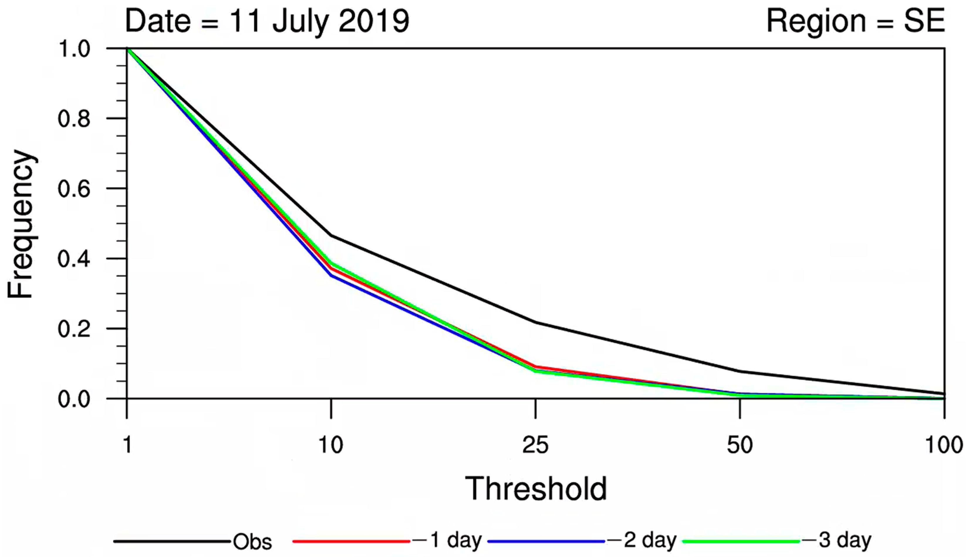
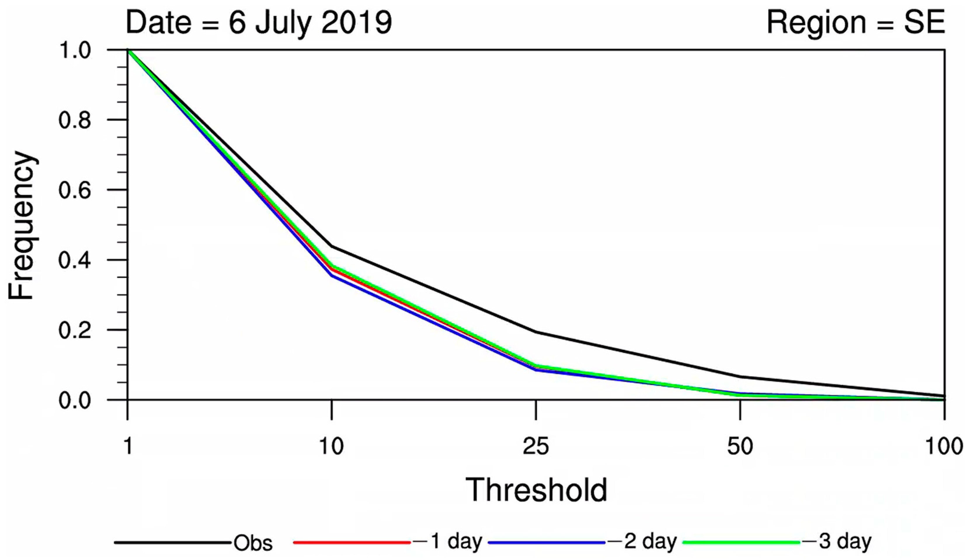
3.1. CDF Statistical Test Analysis

Due to the coarse selection of correction thresholds in this study, which are 1 mm, 10 mm, 25 mm, 50 mm, and 100 mm, the CDF curves of the forecast were located below the observed CDF curve for each threshold. In other words, the forecasted precipitation frequencies for each threshold were lower than the observed precipitation frequencies.
From the observed and forecasted CDF curves for the precipitation event on 11 July 2019 (Figure 1), it can be observed that for precipitation magnitudes below 25 mm, the forecast frequencies were closer to the observed frequencies with a lead time of 3 days. However, for precipitation magnitudes of 25 mm and above, the forecasted precipitation frequencies became closer to the observed values as the lead time decreased.
This observation aligns with previous research findings indicating a common model error, where the frequency of light precipitation is overestimated, while the frequency of heavy precipitation is underestimated. This error becomes more pronounced with longer lead times. This indirectly highlights the necessity of correction for model precipitation forecasts, especially for forecasts with longer lead times.
Compared to the precipitation event on 11 July 2019, the model’s forecasted precipitation frequency curves for various thresholds on July 6th (Figure 2) were closer at different lead times, indicating better forecast stability for this event. However, for both events, the model tended to show significant deviations from the observations, particularly for the 25 mm threshold. This suggests a necessity for correction, especially for moderate to heavy precipitation forecasts.
However, regarding the calculation formula for CCs, the magnitude of the CCs is not only related to the difference between forecasted and observed frequencies, but also to the frequencies corresponding to the corrected magnitude. Therefore, the necessity of correction for heavy rainfall and above still needs to be examined by analyzing the CCs under various correction thresholds.

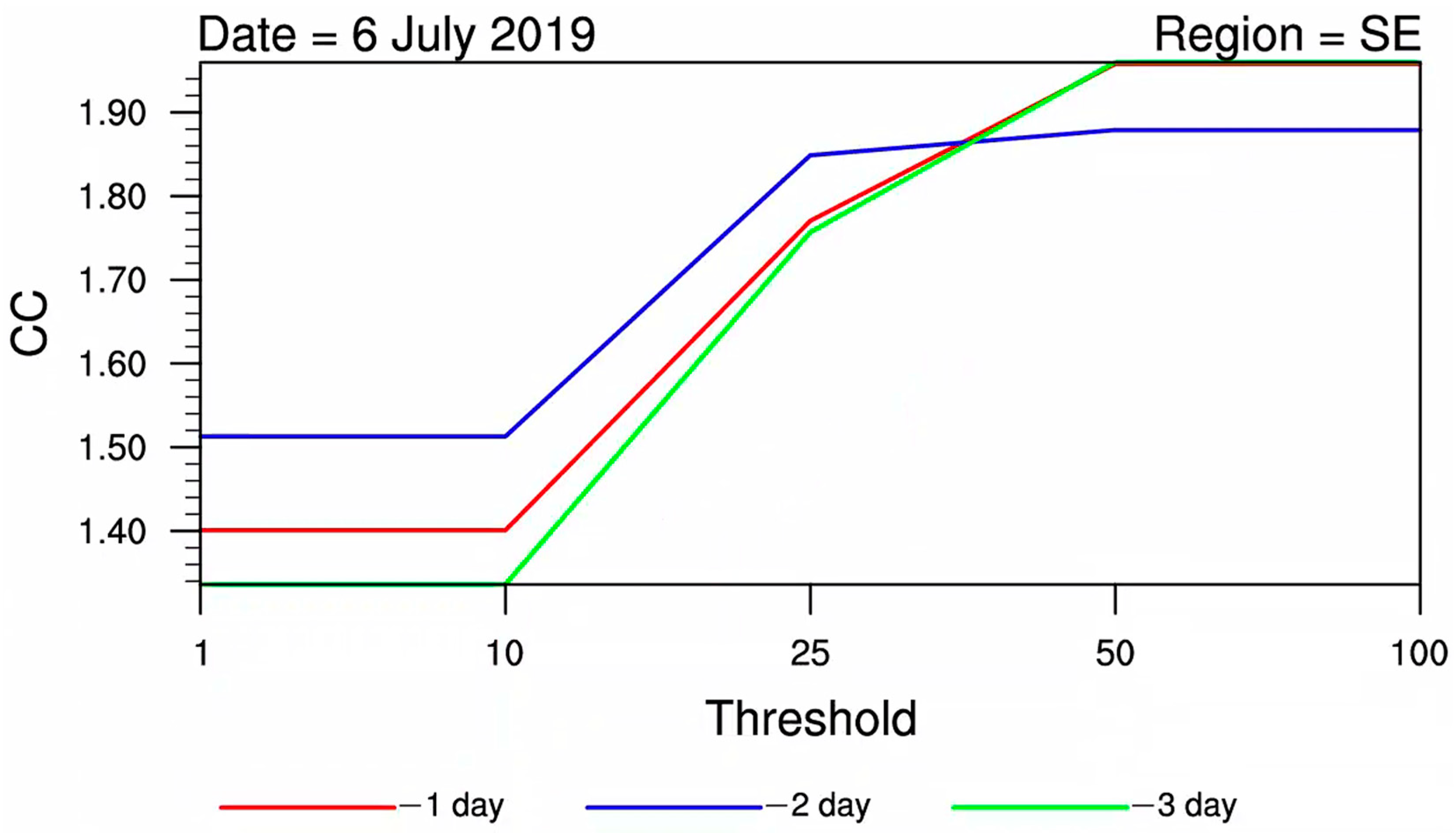
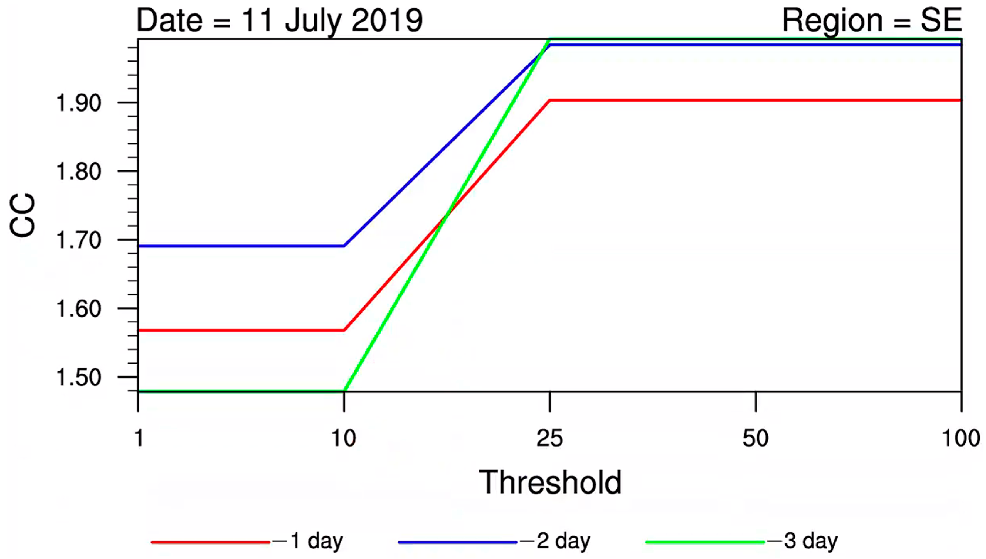
3.2. Correction Coefficient Analysis

Since this correction method can be applied to ensemble forecasts and provides a reference for forecasters to make direct judgments in operational forecasting, it is crucial for the program to use minimal computational resources to ensure smooth operation in operational forecasting and timely provisioning of deterministic forecast information from ensemble forecasts. Therefore, it is necessary to simplify the correction for non-essential precipitation thresholds by examining the CCs for each threshold.
From the analysis of correction coefficient variation curves for different precipitation thresholds at various lead times based on the case study on 11 July 2019 (Figure 3), it can be observed that the CCs increased to varying degrees with increasing precipitation thresholds. Specifically, the CCs for a 1-day lead time were generally smaller than those for a 2-day lead time across all thresholds. Moreover, for a 3-day lead time forecast, the CCs were 0 for thresholds between 1 and 10 mm, but they showed a gradually increasing trend with increasing precipitation magnitudes.
Therefore, it can be preliminarily inferred that as the precipitation magnitude increased and the lead time of the forecast extended, the CCs also increased, indicating a greater necessity for correction.
Similar to the case study on 11 July 2019, the CCs for different lead times increased to varying degrees with increasing precipitation thresholds in the case study on 6 July 2019 (Figure 4). However, for the 1-day lead time forecast, the variation trend of the CCs in the July 5th case study was more pronounced compared to the July 11th case study. This indicates that for the July 5th case study, the CCs for both the 1-day and 3-day lead time forecasts increased more significantly with increasing correction thresholds.
The analysis results for both case studies exhibited similar characteristics: as the precipitation magnitude increased and the lead time of the forecast extended, the CCs also increased, indicating a greater necessity for correction.

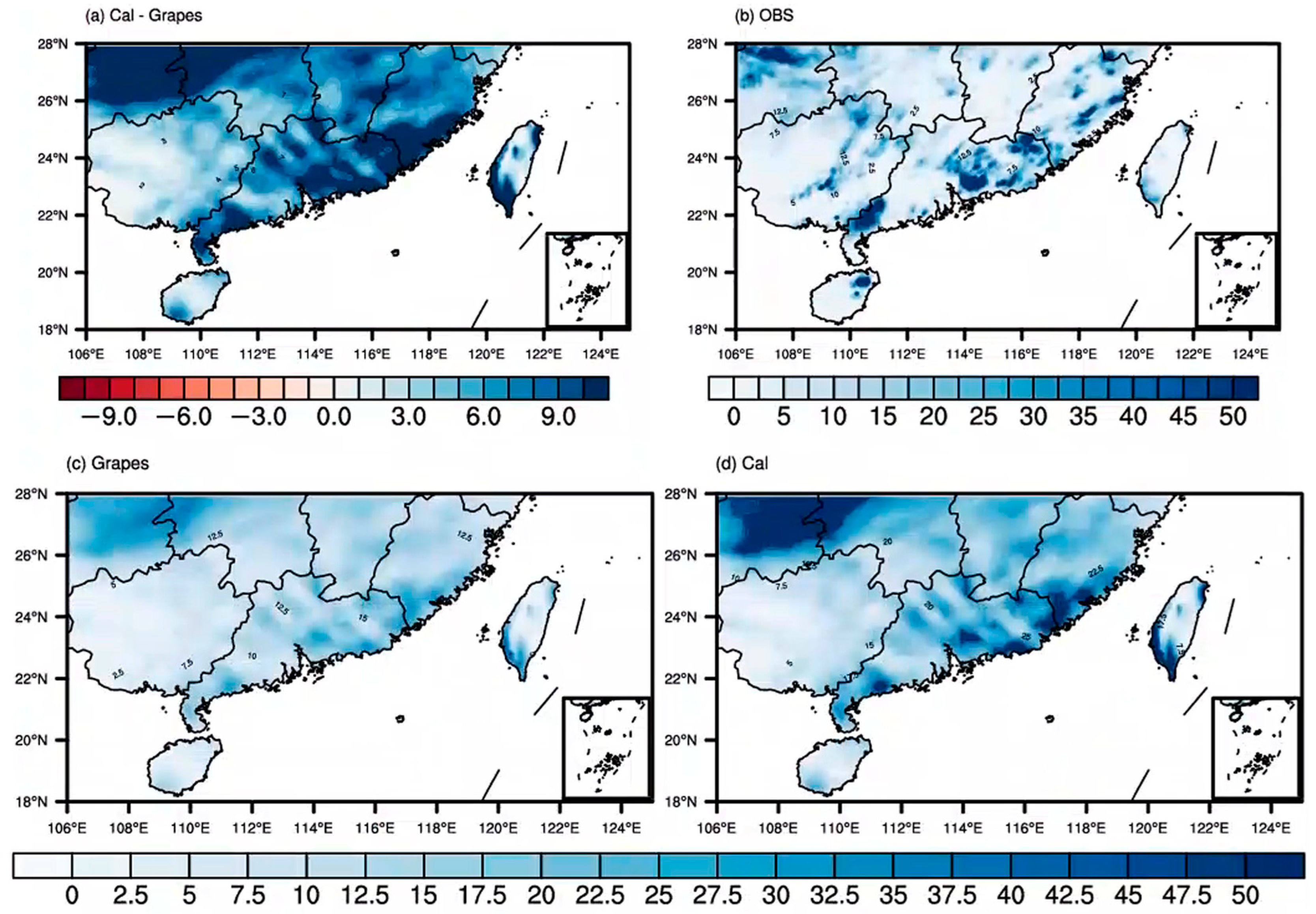
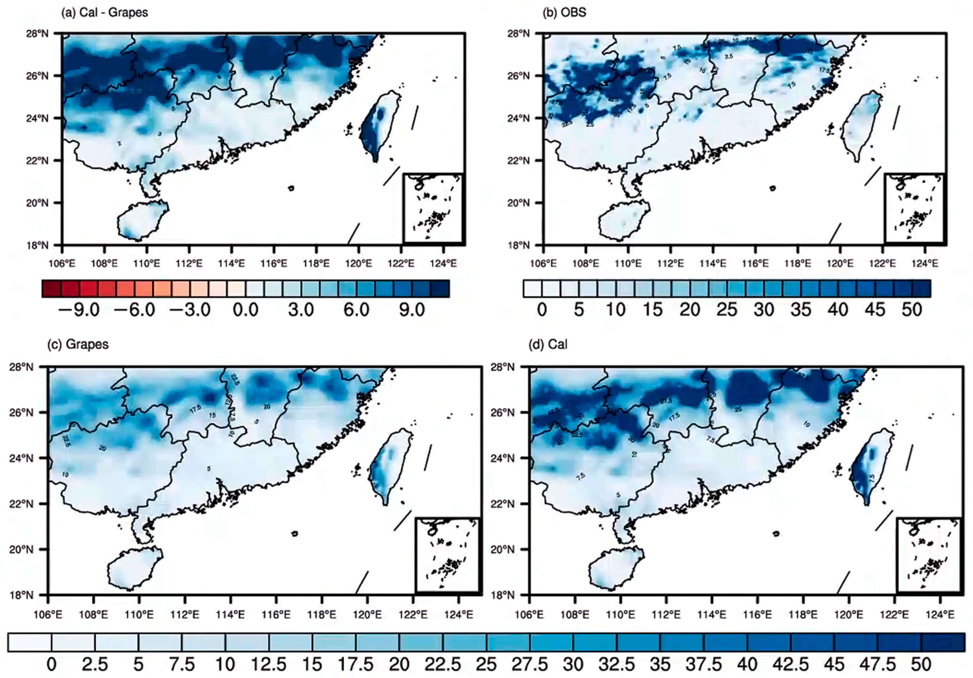
3.3. Comparative Analysis of Precipitation Distribution before and after Correction

Compared to deterministic forecast models, the arithmetic mean forecast of ensemble members in ensemble forecast models tends to have higher accuracy in predicting precipitation distribution. However, a simple arithmetic mean tends to smooth out extreme information in ensemble forecast models, resulting in underestimated precipitation magnitudes. Therefore, when using ensemble forecast models for deterministic forecasting, it is necessary to correct the ensemble mean forecast. The FMM studied in this paper is based on this principle of correction.
To verify the effectiveness of this method in correcting precipitation magnitudes and spatial distribution, the precipitation distributions before and after correction were compared with observations from the selected case studies. An analysis was also conducted before and after correction to evaluate the effectiveness of the correction.
The below figures depict the observed precipitation distribution on 11 July 2019 (Figure 5b), the original model’s 2-day lead time precipitation forecast distribution (Figure 5c), the precipitation forecast distribution after correction (Figure 5d), and the difference in precipitation forecast before and after correction (Figure 5a).
Comparing the observed precipitation distribution with the original model forecast, it is evident that for localized thunderstorms like these, the ensemble mean forecast tends to underestimate precipitation magnitudes due to the smoothing effect of its arithmetic mean. However, the forecasted spatial distribution of precipitation is relatively accurate.
After applying the FMM for correction, the precipitation forecast improved in both spatial distribution and magnitude, closely resembling the observed precipitation. Particularly, for areas along the eastern coast of Guangdong Province, such as Huizhou and Shantou, the forecasted heavy precipitation areas were accurately captured. However, due to resolution issues in model forecasts, there may still be some overestimation errors for heavy precipitation forecasted on the northwest side of South China after correction.
Based on the description provided, for the case study on 6 July 2019 (Figure 6), there was a significant precipitation event in the northern part of South China, primarily affecting northern Guangxi and northern Fujian. The ensemble mean forecast of the model somewhat captured this precipitation event in the northern part of South China, but the forecasted precipitation center was mainly located in the southern part of Hunan Province, resulting in a certain degree of underestimation of the main precipitation area observed.
After applying the frequency matching correction, there was an increase in precipitation magnitudes and an expansion of the heavy precipitation area, making the precipitation forecast closer to the observed values in terms of magnitude. However, there still may be an overestimation bias in the forecasted precipitation for the southern part of the Hunan Province after correction.

4. Quantitative Comparison Analysis before and after Correction

For assessing the effectiveness of deterministic forecasts, there are various evaluation methods available. Since precipitation events are typically binary (either it occurs or it does not), the TS score is commonly used as a metric to evaluate whether precipitation events occur.

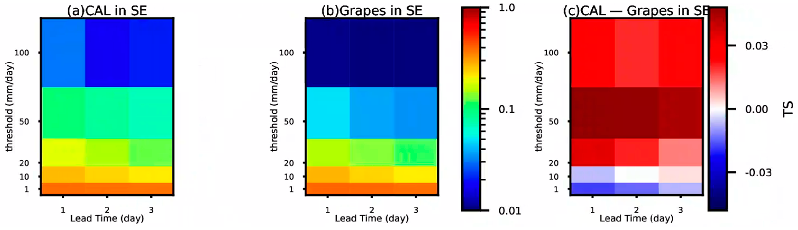
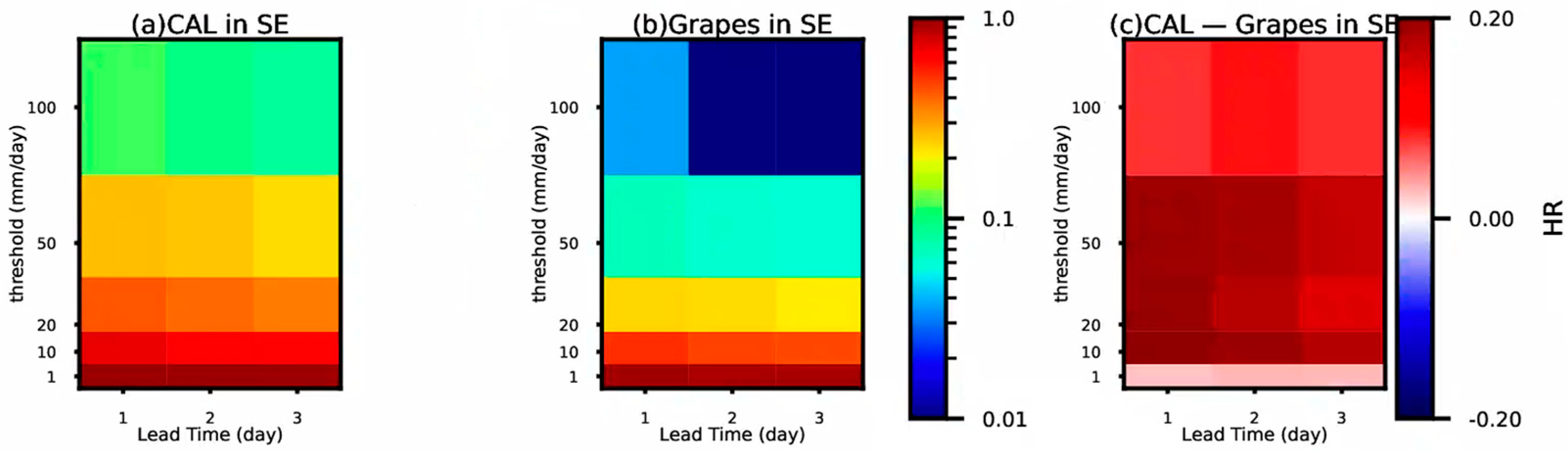
4.1. Comparative Analysis of TS Scores and Hit Rate

The figures below illustrate the TS scores for precipitation forecasts of various magnitudes in the South China region under different lead times, comparing the FMM after correction (Figure 7a) and the ensemble mean of the model before correction (Figure 7b). The colors indicate the TS scores, with blue shades indicating lower scores and red shades indicating higher scores.
For both pre- and post-correction forecasts, as the lead time increased and the precipitation magnitude rose, the TS scores tended to decrease. However, after frequency matching correction, the decrease in TS scores with increasing lead time and precipitation magnitude was less pronounced compared to the ensemble mean.
In comparison, except for the 1–10 mm precipitation magnitude forecasted one day in advance, the TS scores after correction remained unchanged or higher compared to before correction for other precipitation magnitudes and lead times. This suggests that the FMM has an overall positive effect on precipitation forecasts in the South China region, especially for longer lead times and higher precipitation magnitudes, where the correction effect is more significant.
To visually demonstrate the correction effect of the FMM for precipitation forecasts of various magnitudes under different lead times, we subtracted the TS scores after correction from those before correction to obtain the distribution of TS score differences. In the graph (Figure 7c), the horizontal axis represents the lead time, the vertical axis represents the precipitation magnitude, and colors indicate the magnitude of the correction effect, with red indicating a better correction effect, white indicating no correction effect, and blue indicating lower TS scores after correction than before.
From the graph, it is evident that for light rain (1–10 mm), the TS scores after correction were consistently lower than before correction, with a more pronounced negative correction effect as the lead time decreased. Combining this with the TS scores before correction, it can be observed that the ensemble mean forecasts achieved TS scores of 0.35 or higher for light rain, with TS scores reaching 0.4 or higher for a 1-day lead time forecast. This suggests that the ensemble mean forecasts have inherently good predictive performance for light precipitation, possibly due to the smoothing effect of the ensemble mean having a positive predictive effect on light precipitation.
For moderate rain (10–25 mm), the correction initially showed a negative effect for a 1-day lead time forecast, but as the lead time increased, the correction effect gradually became positive, with a positive correction effect observed for a 3-day lead time forecast. For heavy rain (25–50 mm) and torrential rain (50–100 mm), the FMM demonstrated a significant correction effect, with higher TS scores after correction compared to before correction, especially for shorter lead time forecasts.
The TS score is a commonly used metric in operational forecasting to evaluate the performance of precipitation forecasts. However, considering the uncertainty associated with forecasts, additional metrics are required for supplementary analysis. In this study, Hit Rate was utilized to analyze the correction effects of precipitation forecasts (see Figure 8). From the perspective of Hit Rate, the accuracy of the original model forecast (Figure 8b) noticeably decreased with increasing lead time and precipitation intensity. This downward trend was more pronounced than that observed in the TS score, indicating that the decrease in TS score with increasing lead time and precipitation intensity can be mainly attributed to the Hit Rate contribution. After FMM correction, the Hit Rate (Figure 8a) demonstrated a significant improvement compared to the GRAPES model, outperforming the TS score (Figure 8c). This implies that the FMM method enhanced the Hit Rate of precipitation forecasts in the southern region of the GRAPES model, surpassing the TS score. Furthermore, this suggests that the FMM method may result in some overestimation, leading to relatively high false alarm rates (Figure omitted).

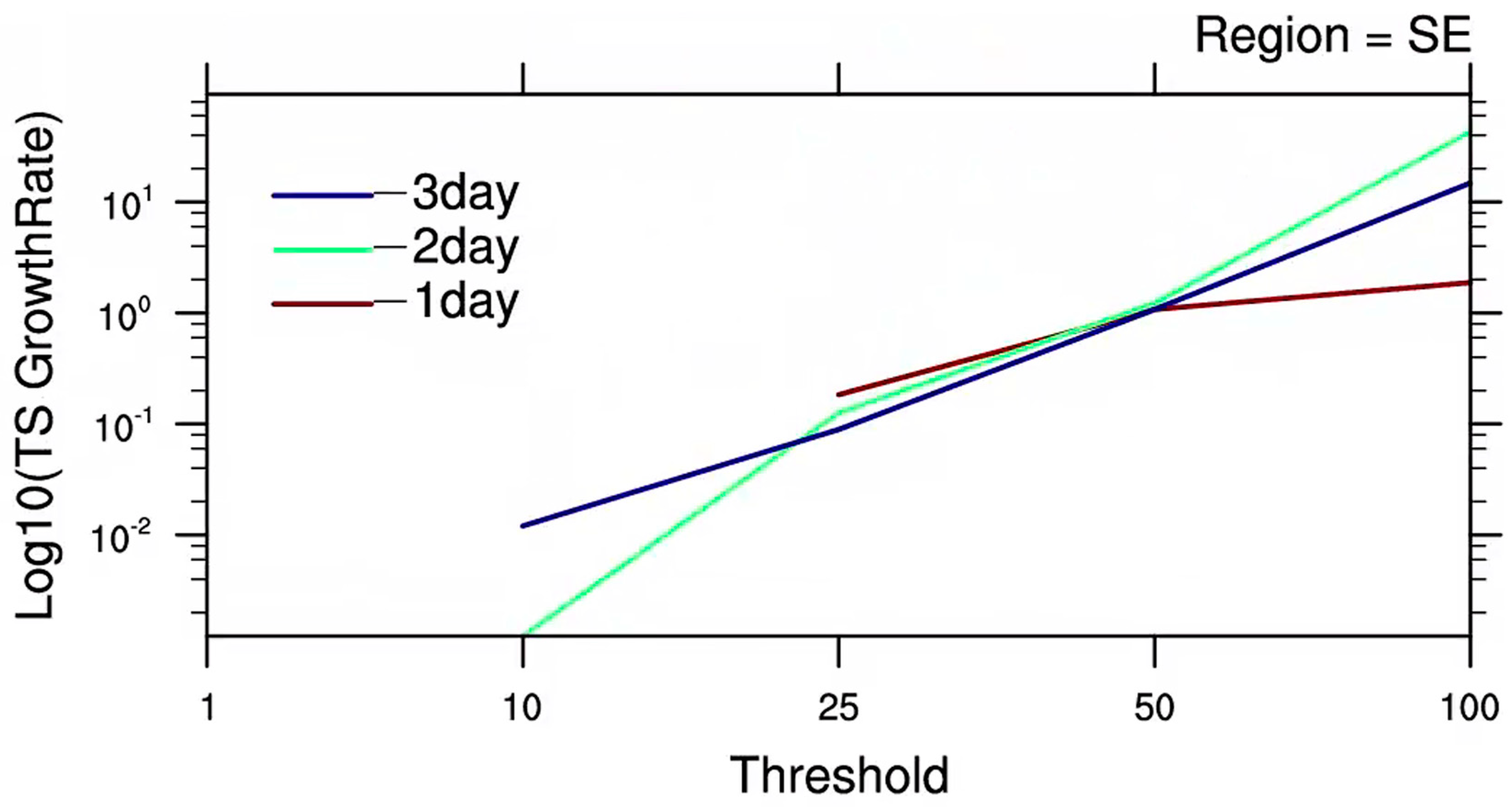
4.2. TS Score Growth Rate

In the above analysis, it was shown that for precipitation magnitudes of heavy rain and above, the correction effect of the FMM is better for forecasts with shorter lead times. However, since subjective correction by forecasters is already optimal for forecasts with shorter lead times, it raises the question of whether the correction effect of the FMM is better for forecasts with shorter lead times for precipitation magnitudes and lead times where a positive correction effect is observed. Further analysis is needed to determine this. Below, we will analyze and present the growth rate of TS scores for forecasts of different precipitation magnitudes under various lead times.
The red, blue, and green curves in the graph below represent the TS score growth rates of frequency-matched precipitation correction forecasts for lead times of 1 day, 2 days, and 3 days, respectively (Figure 9). The values on the vertical axis are the logarithm of the growth rates. Precipitation magnitudes where frequency matching had a negative correction effect for the respective lead times are not shown in the graph.
It can be observed that the TS score growth rate curves for each lead time are displayed for precipitation magnitudes of 25 mm and above, indicating that the FMM has a certain correction effect on heavy rain and above precipitation magnitudes. All curves show an increasing trend as the precipitation magnitude increases, with the trend becoming more pronounced for longer lead times. This suggests that for heavier precipitation magnitudes, there is a greater necessity for frequency matching correction, and the correction effect becomes more significant with longer lead times.

5. Discussion and Conclusions

The study utilized real-time forecast products from the GRAPES_MESO regional ensemble forecast model developed by the China Meteorological Administration’s National Meteorological Center, with forecasts issued 12 h in advance for lead times of 1–3 days. These forecasts were combined with homogenized precipitation grid data from national-level surface meteorological stations as observational data. The FMM was applied to correct precipitation forecasts for light rain, moderate rain, heavy rain, and torrential rain magnitudes. Comparative analysis was conducted through case studies and statistical tests (TS scores) to evaluate the forecast performance before and after correction. The following conclusions were drawn:
(1)
The model’s CDF curves exhibited deviations compared to observations, with the discrepancies becoming more pronounced with longer lead times. Therefore, the necessity for correction of model precipitation forecasts, especially for longer lead times, is apparent.
(2)
The CCs showed a gradually increasing trend with higher precipitation magnitudes, indicating that as the precipitation magnitude increases and the lead time extends, the necessity for correction becomes more significant.
(3)
Analysis of two precipitation cases in Southern China in July 2019 revealed through frequency matching correction that as precipitation magnitudes increase, the range of heavy rainfall expands. After frequency matching correction, the precipitation forecasts became more aligned with observations in terms of magnitude.
(4)
Statistical tests using TS scores demonstrated that frequency matching correction has a certain corrective effect on precipitation forecasts in Southern China overall, particularly for forecasts with longer lead times and higher precipitation magnitudes, where the correction effect was more pronounced.
(5)
Frequency matching correction showed a certain corrective effect for heavy rainfall and above magnitudes of precipitation. Additionally, for shorter lead times, the TS scores after correction were higher compared to before correction.
(6)
The necessity for frequency matching correction becomes more apparent for heavier precipitation events. Furthermore, the correction effect becomes more pronounced with longer lead times.

Author Contributions

Conceptualization, H.C.; methodology, J.Z.; software, X.Z.; validation, D.Y. and L.W.; formal analysis, J.D.; investigation, J.Z.; resources, H.C.; data curation, J.D.; writing—original draft preparation, J.Z.; writing—review and editing, J.D.; visualization, J.Z.; supervision, H.C.; project administration, J.D.; funding acquisition, H.C. All authors have read and agreed to the published version of the manuscript.

Funding

This research was jointly funded by the National Key Research and Development Program of China (2021YFC3000902) and the National Natural Science Foundation of (U20A2097, 42075087).

Institutional Review Board Statement

Not applicable.

Informed Consent Statement

Not applicable.

Data Availability Statement

The GRAPES Ensemble Forecast Product was obtained from the Earth System Modeling and Prediction Center with the permission of China Meteorological Administration, China’s National Surface Meteorological Station Normalized Precipitation Daily Value Data Set (V1.0) can be obtained from the China Meteorological Data Service Centre at https://data.cma.cn (accessed on 28 February 2024).

Acknowledgments

All figures were created using the NCAR Command Language (NCL) (2021), http://www.ncl.ucar.edu (accessed on 28 October 2023).

Conflicts of Interest

The authors declare no conflicts of interest.

References

  1. Du, J.; Kang, Z.M. A Survey on Forecasters’ View about Uncertainty in Weather Forecasts. Adv. Meteorol. Sci. Technol. 2014, 4, 58–67. [Google Scholar]
  2. Wei, M.Z.; Toth, Z.; Wobus, R.; Zhu, Y. Initial perturbations based on the ensemble transform (ET) technique in the NCEP global operational forecast system. Tellus A 2008, 60, 62–79. [Google Scholar] [CrossRef]
  3. Houtekamer, P.L.; Mitchell, H.L. Ensemble Kalman filtering. Q. J. R. Meteorol. Soc. 2005, 131, 3269–3289. [Google Scholar] [CrossRef]
  4. Houtekamer, P.L.; Charron, M.; Mitchell, H.L.; Pellerin, G. Status of the global EPS at environment Canada. In Proceedings of the ECMWF Workshop on Ensemble Prediction, Reading, UK, 7–9 November 2007; ECMWF: Reading, UK; pp. 57–68. [Google Scholar]
  5. Zhou, X.Q.; Zhu, Y.J.; Hou, D.C.; Kleist, D. A comparison of perturbations from an ensemble transform and an ensemble Kalman filter for the NCEP global ensemble forecast system. Weather Forecast. 2016, 31, 2057–2074. [Google Scholar] [CrossRef]
  6. Zhu, Y.J.; Li, W.; Zhou, X.Q.; Hou, M. Stochastic Representation of NCEP GEFS to Improve Sub-Seasonal Forecast; Springer Atmospheric Sciences; Springer: Singapore, 2019; pp. 317–328. [Google Scholar]
  7. Epstein, E.S. Stochastic dynamic prediction. Tellus 1969, 21, 739–759. [Google Scholar] [CrossRef]
  8. Leith, C.E. Theoretical skill of Monte Carlo forecasts. Mon. Weather. Rev. 1974, 102, 409–418. [Google Scholar] [CrossRef]
  9. Palmer, T.N.; Brankovic, C.; Richardson, D.S. A probability and decision-model analysis of PROVOST seasonal multi-model ensemble integrations. Q. J. R. Meteorol. Soc. 2000, 126, 2013–2033. [Google Scholar]
  10. Richardson, D.S. Skill and relative economic value of the EC-MWF ensemble prediction system. Q. J. R. Meteorol. Soc. 2000, 126, 649–668. [Google Scholar] [CrossRef]
  11. Wang, R.; Liang, Y.; Cai, H.; Zheng, J. Ability of the GRAPES Ensemble Forecast Product to Forecast Extreme Temperatures over the Tibetan Plateau. Atmosphere 2023, 14, 1625. [Google Scholar] [CrossRef]
  12. Ren, P.; Gao, L.; Zheng, J.; Cai, H. Key Factors of the Strong Cold Wave Event in the Winter of 2020/21 and Its Effects on the Predictability in CMA-GEPS. Atmosphere 2023, 14, 564. [Google Scholar] [CrossRef]
  13. Cai, H.; Zhao, Z.; Zheng, J.; Luo, W.; Li, H. Evaluation of the Dynamical–Statistical Downscaling Model for Extended Range Precipitation Forecasts in China. Atmosphere 2022, 13, 1663. [Google Scholar] [CrossRef]
  14. Zheng, J.; Ren, P.; Chen, B.; Zhang, X.; Cai, H.; Li, H. Research on a Clustering Forecasting Method for Short-Term Precipitation in Guangdong Based on the CMA-TRAMS Ensemble Model. Atmosphere 2023, 14, 1488. [Google Scholar] [CrossRef]
  15. Wu, M.; Luo, Y.; Chen, F.; Wong, W.K. Observed link of extreme hourly precipitation changes to urbanization over coastal South China. J. Appl. Meteor. Climatol. 2019, 58, 1799–1819. [Google Scholar] [CrossRef]
  16. Du, J.; Mullen, S.L.; Sanders, F. Short-range ensemble forecasting of quantitative precipitation. Mon. Weather. Rev. 1997, 125, 2427–2456. [Google Scholar] [CrossRef]
  17. Ebert, E.E. Ability of a poor man’s ensemble to predict the probability and distribution of precipitation. Mon. Weather. Rev. 2001, 129, 2461–2480. [Google Scholar] [CrossRef]
  18. Li, L.; Zhu, Y.J. The Establishment and Research of T213 Precipitation Calibration System. J. Appl. Met. Eorological. Sci. 2006, 17, 130–134. [Google Scholar]
  19. Li, J.; Du, J.; Chen, C.J. Introduction and Analysis to Frequency or Area Matching Method Applied to Precipitation Forecast Bias Correction. Meteorol. Mon. 2014, 40, 580–588. [Google Scholar]
  20. Li, J.; Du, J.; Chen, C.J. Applications of “Frequency-Matching” Method to Ensemble Precipitation Forecasts. Meteorol. Mon. 2015, 41, 674–684. [Google Scholar]
  21. Li, W.; Duan, Q.; Miao, C.; Ye, A.; Gong, W.; Di, Z. A review on statistical post processing methods for hydro meteorological ensemble forecasting. WIREs Water 2017, 4, e1246. [Google Scholar] [CrossRef]
  22. Duan, Q.; Pappenberger, F.; Wood, A.; Cloke, H.L.; Schaake, J.C. Hand-Book of Hydrometeorological Ensemble Forecasting; Springer: Berlin/Heidelberg, Germany, 2020. [Google Scholar]
  23. Shahi, N.K.; Polcher, J.; Bastin, S.; Pennel, R.; Fita, L. Assessment of the spatio-temporal variability of the added value on precipitation of convection-permitting simulation over the Iberian Peninsula using the RegIPSL regional earth system model. Clim. Dyn. 2022, 59, 471–498. [Google Scholar] [CrossRef]
  24. Shahi, N.K.; Rai, S.; Sahai, A.K.; Abhilash, S. Intra-seasonal variability of the South Asian monsoon and its relationship with the Indo–Pacific sea-surface temperature in the NCEP CFSv2. Int. J. Climatol. 2018, 38, e28–e47. [Google Scholar] [CrossRef]
Figure 1. CDF distribution curves for various lead time days on 11 July 2019.
Atmosphere 15 00466 g001
Figure 2. CDF distribution curves for various lead times (in days) on 6 July 2019.
Atmosphere 15 00466 g002
Figure 3. Distribution curve of CCs for various lead time (in days) on 11 July 2019.
Atmosphere 15 00466 g003
Figure 4. Distribution curve of CCs for various lead times (in days) on 5 July 2019.
Atmosphere 15 00466 g004
Figure 5. Distribution of correction zone (a), actual precipitation (b), original forecast (c), corrected forecast (d) for a lead time of 2 days on 11 July 2019.
Atmosphere 15 00466 g005
Figure 6. Distribution of correction zone (a), actual precipitation (b), original forecast (c), corrected forecast (d) for a lead time of 1 day on 6 July 2019.
Atmosphere 15 00466 g006
Figure 7. TS scores before (a) and after (b) correction, and distribution of TS score differences before and after correction (c).
Atmosphere 15 00466 g007
Figure 8. Same as Figure 7, but for Hit Rate.
Atmosphere 15 00466 g008
Figure 9. Logarithmic plot of TS growth rate before and after correction.
Atmosphere 15 00466 g009
Table 1. Precipitation Verification Classification Table.
ObservationPrecipitation
Occurs
No
Precipitation
Forecast
Precipitation OccursNANB
No PrecipitationNCND
Disclaimer/Publisher’s Note: The statements, opinions and data contained in all publications are solely those of the individual author(s) and contributor(s) and not of MDPI and/or the editor(s). MDPI and/or the editor(s) disclaim responsibility for any injury to people or property resulting from any ideas, methods, instructions or products referred to in the content.

