Abstract
Aircraft and rockets entered the lower stratosphere on a regular basis during World War II and have done so in increasing numbers to the present. Atmospheric testing of nuclear weapons saw radioactive isotopes in the stratosphere. Rocket launches of orbiters are projected to increase substantially in the near future. The burnup of orbiters has left signatures in the aerosol. There are proposals to attenuate incoming solar radiation by deliberate injection of artificial aerosols into the stratosphere to “geoengineer” cooling trends in surface temperature, with the aim of countering the heating effects of infrared active gases. These gases are mainly carbon dioxide from fossil burning, with additional contributions from methane, chlorofluorocarbons, nitrous oxide and the accompanying positive feedback from increasing water vapor. Residence times as a function of altitude above the tropopause are critical. The analysis of in situ data is performed using statistical multifractal techniques and combined with remotely sensed and modeled results to examine the classical radiation–photochemistry–fluid mechanics interaction that determines the composition and dynamics of the lower stratosphere. It is critical in assessing anthropogenic effects. It is argued that progress in predictive ability is driven by the continued generation of new and quantitative observations in the laboratory and the atmosphere.
1. Introduction
This paper is organized to provide a condensed history of how the lower stratosphere is supplied with air and molecular content, both natural and anthropogenic. The central importance of new, accurate, original measurements and observations, both in the laboratory and the atmosphere, emerges as a central theme. Such measurements have addressed issues about the composition, photochemistry and radiative balance of the region. The results from the original work on the lower stratosphere resulted in the following picture. Air moving upwards from the troposphere enters the stratosphere across the tropopause in the tropics [1,2,3], with some entering the lower stratosphere at midlatitudes via the subtropical jet stream and polar front jet streams connected with cyclonic development [4,5] and cumulonimbus activity [6]. Downward-moving air leaving the lower stratosphere does so mainly in extratropical latitudes, by tropopause folding [7,8,9], with some contribution from radiatively driven descent. The low latitude exchange between the lower subtropical stratosphere and the upper tropical troposphere, via collapsing cumulonimbus and isentropic transfer equatorward from the subtropical jet stream, leads to detectable fractions of stratospheric air in the troposphere above 12–14 km altitudes up to the tropical tropopause at about 16–17 km altitude [10,11].
The circulation in the extratropical lower stratosphere was determined to have westerly winds in the winter and easterlies in the summer [12]. It was further determined to have a cyclonic winter polar vortex in the Arctic up to at least 50 mbar [13].
The 1963 eruption of Mt. Agung revealed that sufficiently energetic volcanic events could penetrate the tropopause and spread worldwide [14,15]. It injected a large volume of sulfurous aerosol, which exerted detectable radiative effects on the lower stratosphere, causing local heating in the lower stratosphere [16] and a smaller cooling in the surface air. An aerosol layer at 15-20 km, the Junge Layer, was detected by balloon-borne sondes [17]. The realization that the radioactive fallout clouds from nuclear explosions ≥1 megaton yield in the 1950s and 1960s stabilized in the lower stratosphere [18] led to an increase in both measurement and modeling activities. Studies of radioactivity, volcanic ejecta and later, of gases indicated that residence times ranged from days to a few weeks in the 3–5 km above the tropopause to about 5–6 years in the upper stratosphere. Descent in the winter polar vortex was an important process in transporting air from the mesosphere and upper stratosphere into the lower stratosphere.
With the advent of jet aircraft and rocket launches, engine exhaust emissions were emitted into the lower stratosphere. Burnup of satellite payloads on re-entry produces particulate matter that descends in the winter polar vortex to the lower stratosphere. Such anthropogenic emissions have the potential to affect the chemical and radiative balance of the region.
A recurring theme is that new quantitative measurements, both in the laboratory and the atmosphere, have a major impact in that generally, they have led to new results that were largely not initially forecast by modeling efforts. Examples are the effects of reactive, short-lived halogenated molecules on the ozone concentration; the measurements of rocket exhausts after launch reducing ozone by greater amounts than calculated and the enhanced effects on the radiative balance of the observed water mixing ratios.
2. Observed State via In Situ Methods
The bottom 5 km or so above the northern midlatitude tropopause has a signature of air that has not been dried exclusively at the tropical tropopause, see Figure 1. It is particularly evident in the lowermost stratosphere, just above the tropopause. This is a modern version of what was seen originally at northern midlatitudes in Ref. [3] and later in Ref. [4].
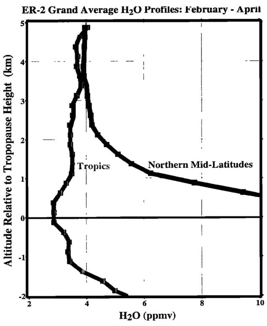
Figure 1.
Average water vapor profiles in the tropics and in northern midlatitudes during the late winter/spring period when the tropical tropopause is coldest. The data are from ER-2 take-offs and landings 1987–1996 at Darwin and Panama (tropics), and from Moffett Field; Bangor, Maine and Wallops Island (midlatitudes). It is apparent that the air in the lowest 5 km above the tropopause has not been dried exclusively in the tropics. After Ref. [19].
It had been established, by using a frost point hygrometer modified to work with CO2 instead of H2O [3], that there was no gravitational separation by molecular weight in the lower stratosphere.
A central fact of stratospheric ozone is its vertical distribution and the causes underlying it. Solar ultraviolet radiation photodissociates molecular oxygen at wavelengths below 242 nm, resulting in oxygen atoms that recombine with oxygen molecules to produce ozone. The wavelengths below 242 nm do not penetrate beyond the upper stratosphere, and chain reactions involving HOx, NOx and ClO free radicals destroy ozone catalytically. The net result is a maximum in ozone number density, which means that most of the UV-absorbing activity occurs below about 25 km, depending on latitude. Figure 2 shows typical examples. Basic mechanisms are shown in Figure 3.
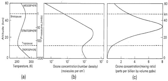
Figure 2.
(a) Typical temperature profile. (b) Typical ozone number density profile. (c) Typical mixing ratio profile. The contrast between (b,c) shows why the greatest contributions to the total overhead ozone column arise from altitudes below 25 km, depending on latitude; the number density profile shows where the greatest contribution to the overhead column amount is located. The maxima in the profiles in (b,c) slope downwards from the tropics toward the poles. Profiles of DU (Dobson Units) per km are in Figure 4 of Ref. [20].
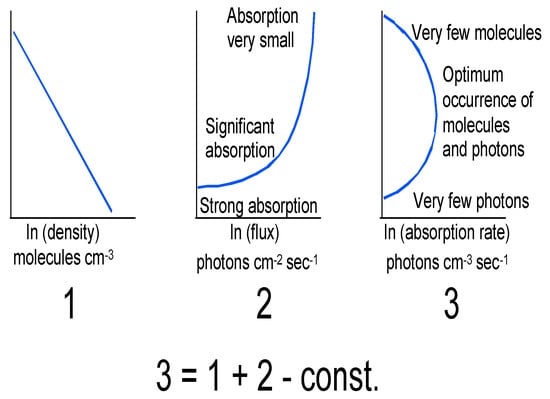
Figure 3.
(1) is the logarithmic density profile. (2) is the solar flux and (3) is the resulting absorption rate to produce ozone. The result is a mixing ratio profile peaking at about 30 km, while the number density profile peaks lower down at about 20–25 km in midlatitudes, see Figure 2. After Ref. [21].
By 1970, theories had been promulgated that the missing sink to account for the excess ozone calculated in the stratosphere by use of the pure oxygen Chapman reactions [22,23] could be chain reactions involving OH and HO2 [24,25,26] or NO and NO2 [27,28,29]. In both cases, it was proposed that the reaction of the excited O(1D) atom from ozone photodissociation with the stable parent molecules H2O and N2O was the source of two OH and two NO reactive molecules, respectively. There was one report of these odd nitrogen species in the stratosphere, an observation of NO and HNO3 nitric acid vapor [30].
3. The Period of 1971–1984
The catalytic chain reactions meant that species at mixing ratios three or four orders of magnitude less than that of ozone could, via chain lengths of 104, significantly attenuate the ozone layer. Two papers in 1971 changed the landscape regarding anthropogenic effects in the lower stratosphere [31,32]. The proposed Boeing 2707 and the Anglo-French Concorde supersonic airliners would fly well into the stratosphere, and chemical kineticists led by Harold Johnston did some quick calculations that suggested that 500 2707s would cause significant losses in the ozone layer via the NO emitted by their exhausts. The combustion chambers were hot enough to make the major air constituents N2 and O2 react to produce NO at about 1% mixing ratio via the following possible, much simplified, reaction sequence:
O2 + M → O + O + M
O + N2 → N + NO
N + NO → N2 + O
NO + O2 → O + NO2
NO + NO + O2 → NO2 + NO2
These reactions involve reactants that have excited states, electronic in all cases and vibrational and rotational in the case of molecules. At temperatures reached in jet engines, ionization is not significant, but it is in lightning and nuclear weapon explosions. In the latter cases, the ionized air ranges from temperatures of approximately 30,000 K to 7000 K, at which point, the cooling air becomes transparent to visible radiation [33]. The temperature at which significant production of NO occurs is about 2000 K and above. The radius of the shocked air at 2000 K is larger than that at 7000 K, so the shock wave produces more NO than the ionized channel [34,35]. When water is included, significant production of OH and HO2 also occurs [36] because the dissociation of H2O occurs at about the same temperatures (>2100 K) as (R1), the initiator of the chain reaction (R2), (R3), which mainly produces NO [33]. Lightning has recently been observed to produce fine aerosols too [37]. The exhaust emission of Concorde has been measured directly in the lower stratosphere and includes particulates as well as the gaseous species [38].
A Nobel Prize-winning paper was published in 1974 [39], which pointed out that the chlorine atoms liberated from chlorofluoromethanes could destroy ozone once they were transported above the ozone maximum. These molecules were widely used as refrigerants and propellants and were growing exponentially. The paper was based on measurements of CFCl3 and CF2Cl2 over extensive areas of the planetary surface [40]. The liberation of free chlorine atoms by UV photodissociation above the ozone maximum was calculated to destroy the ozone by the following chain reaction:
X + O3 → XO + O2
XO + O → X + O2
nett: O + O3 → O2 + O2
XO + O → X + O2
nett: O + O3 → O2 + O2
The time taken to circulate the entire atmospheric content of the chlorofluoromethanes above the ozone maximum resulted in very long lifetimes for these molecules, which had no other detectable sink. The current values are 52 and 102 years for CFCl3 and CF2Cl2, respectively [41]. Chain lengths can extend to 104, making it possible for parts per billion of X to destroy parts per million of odd oxygen, O + O3 [42].
The first critical test of the theory was when X ≡ Cl came with balloon observations of ClO in the stratosphere [43]. Further consistency was gained by measurements of HCl [44,45,46,47] and of total chlorine and bromine [48]. Laboratory studies of diatomic free radicals were extended to BrO [49] following the authors’ earlier work on ClO that had underpinned [39]. Nitrous oxide had been detected in the earth’s atmosphere by IR spectroscopy just after WW2 [50]. N2O and CH4 had been shown to decrease above 15 km by spectroscopic methods, see Table 1 of Ref. [51]. Whole air sampling from balloons confirmed that vertical profiles of CFCl3, CF2Cl2 and N2O decreased with altitude in the stratosphere [52,53], the product of two factors including the operation of stratospheric sink processes and the ongoing growth in the troposphere as the result of continuing production at the surface, which was much larger for the chlorofluoromethanes than for nitrous oxide. Nitrous oxide is naturally produced by bacterial action in soils [54]. Agriculture has caused a persistent increase over the past several decades.
Cross-coupling between the HOx and NOx chains was realized [32], and the need to include ClOx chain reactions was proposed to be significant [55,56]. The complexity of the reactions involved is laid out in chapter 5 of Ref. [57]. Measurements of some hydrogen-oxygen–nitrogen molecules in the stratosphere [58] eventually turned into a test of the photochemical models, revealing a large problem with calculations of the NO2/HNO3 ratio [59,60]. The state of stratospheric chlorine photochemistry was reviewed [61]. At that stage, the photochemistry considered had been entirely homogeneous gas phase kinetics, with no account of any heterogeneous reactions on aerosol surfaces. That was about to change.
A significant event with future ramifications was the detection of clouds in the winter stratospheric polar vortices by the SAGE II satellite [62], at temperatures significantly warmer than the frost point for water vapor. These were identified as “polar stratospheric clouds” (PSCs) shortly afterward [63].
A thorough review of the state of play up to 1981 is available Ref. [64]. In it, Figure 6 shows in two dimensions, pole to pole, what Figure 2 above shows in one. One-dimensional, column, 1D coordinates had been the focus, but it was realized that a wider context was needed. Accordingly, a 2D, latitude–height, study was performed, which was the best that could be attempted with the contemporary computer power and data availability. Overall, 82% of the ozone was below 10 mbar (30 km), with more in the winter hemisphere and lower down. At the time, it was not possible to represent the polar vortex including chemistry accurately. The winter polar vortex was persistently calculated by general circulation models to have a large cold bias compared with observations [65]. Of course, it was not possible for two-dimensional models to represent well the pathologically three-dimensional vortex.
It was realized that the ozone photochemistry and the radiative effects of carbon dioxide increases from fossil fuel burning were interactive, particularly in the upper stratosphere [42,65]. One early general circulation model prediction was that the Indian Ocean Southern Hemisphere summer monsoon transported significant amounts of upper tropospheric air into the lower stratosphere of the Southern Hemisphere [66,67]. That would later turn out to be a significant effect with its Northern Hemisphere equivalent once satellite observations were available; it provides a route for upper tropical tropospheric air to enter the midlatitude lower stratosphere. The interaction of the three maxima in the subtropical jet stream with stratospheric anticyclones was significant in both hemispheres in a diagnosis made in January.
The necessary three-dimensional model approach was applied and analyzed in the early 1980s. The major dynamical event that occurs in approximately one year of three in the Northern Hemisphere winter stratosphere, Sudden Stratospheric Warmings, was spontaneously produced in a general circulation model and linked to cyclogenesis in the troposphere [68,69]. Observationally based analyses of the entry of air to the stratosphere [70] and exchange across the tropopause [71,72] were also published. References [64,66,71] contain citations of several investigations that are reflective of the state of knowledge at the time.
Two observational papers that, in hindsight, had important predictive power but were underappreciated at the time involved NO2 observations from a ship [73,74]. The term “Noxon Cliff” was used to describe the sharp gradient in stratospheric NO2 between mid- and Antarctic latitudes, with very low values poleward. It indicated that there was an unknown sink process operating at high southern latitudes, a discovery that was portentous.
4. The Period of 1985–2006
In 1985, a paper was published that revolutionized the photochemical understanding of the stratosphere, by extending the study of the summer ozone column over Antarctica [75] to the late winter and spring [76]. The Halley Bay observations [76] of large depletions in the ozone column in the winter polar vortex were extended by analysis of the TOMS (Total Ozone Mapping Spectrometer) instrument’s observations from the Nimbus 7 satellite [77]. Those low values were discounted because the low ozone columns seen over Antarctica in late winter and early spring were below the threshold of what had been deemed possible. The satellite observations showed the depletion to be vortex-wide and gave rise to the “ozone hole” description [77].
The original prediction [39] was for reductions of about 10% located in the upper stratosphere at low and midlatitudes by the late 21st Century; what had occurred was reductions exceeding 50% in the lower Antarctic stratosphere starting apparently in October 1977. It was clear that conventional gas-phase photochemistry could not account for the loss. Several theories were proposed to explain the ozone hole; the one that eventually proved to be successful involved heterogeneous chemistry on the surface of polar stratospheric particles [78], which liberated reactive chlorine atoms and molecules from the reservoir species. Freed from ClONO2 and HCl, the Cl2 rapidly photodissociated, with the Cl atoms producing ClO by reaction with ozone. The self-reaction of ClO to produce Cl2O2 was the rate-determining step of the operative chain reaction [79,80], with BrO also active to a lesser extent. The involvement of polar stratospheric clouds (PSCs) was posited as active in the production of HNO3 at Arctic latitudes [81], and their presence was confirmed by analysis of anomalous radiances by the Limb Infra-red Monitor of the Stratosphere (LIMS) instrument on the Nimbus 7 satellite [82]. In turn, [82] inspired [83], which determined that nitric acid trihydrate crystals could form at PSC temperature and pressure.
Strong indications of perturbed photochemistry were observed in the springtime Antarctic vortex by the first National Ozone Experiment (NOZE-I) expedition from McMurdo in 1986 [84,85,86]. The abundance and diurnal behavior of OClO could not be explained by currently employed photochemical mechanisms, as was true of NO2 and O3. Ozonesonde ascents from McMurdo and the South Pole showed that the ozone loss was concentrated in the lower stratosphere, between 10 and 25 km [87,88]. In 1987, the National Aeronautics and Space Administration–National Oceanic and Atmospheric Administration–National Science Foundation–United Kingdom Meteorological Office–European Centre for Medium-Range Weather Forecasts (NASA-NOAA-NSF-UKMO-ECMWF) Airborne Antarctic Ozone Experiment (AAOE) flew, in late August and through September, in situ instruments on the high-altitude ER-2 and remote sounding instruments plus in situ ozone and total water on DC-8, at 16–20 and 10–12 km, respectively [89]. The flights ranged from Punta Arenas (53° S, 71° W) south to 72° S (ER-2) and to the pole (DC-8).
The immediate results from the ER-2 were that the vortex was dehydrated [90], denitrified [91] with direct detection of PSC particles containing reactive nitrogen [92], with high ClO [93,94,95] leading to small amounts of ozone depletion in late August to large losses in late September [96,97]. Tracer measurements showed large depletions of N2O [98], CFCl3 and CF2Cl2 [99]. The tracers thus indicated substantial descent in the vortex, with air having been brought down from the sink regions above the ozone maximum. The synoptic-scale activity caused poleward moving ridges in the upper troposphere and lower stratosphere that forced PSCs in the vortex and promoted transport to midlatitudes; the vertical region in the lowermost stratosphere between 400 K potential temperature and the tropopause at 300 K had a freer exchange with midlatitudes than did the overlying vortex [100].
The realization that there was ozone loss at the periphery of the Antarctic vortex, occurring in the air with temperatures exposures that were observed within the Arctic vortex, led to a further aircraft mission, the Airborne Arctic Stratospheric Expedition (AASE) [101]. An important result was the measurement from the ER-2 of ClO mixing ratios at the center of the Arctic vortex in mid-February 1989 [102], which were as high as those in the Antarctic in August/September 1987, some 1200 pptv. It was also established that there was a vertical redistribution of NOy. following the detection of elevated levels from the DC-8 that had descended under gravity in PSC particles from ER-2 altitudes and then evaporated [103]. PSC formation and behavior was characterized and calculated in more detail [104,105,106]. Their radiative effects [107] and chemical consequences [108,109] were calculated. The exchange between the vortex and midlatitudes was observed, driven by underlying tropospheric cyclogenesis, with tropospheric air seen up to 420 K potential temperature [100,110]. The age of air from stratospheric entry at the tropical tropopause to descent in the winter vortex was deduced from CO2 observations from the ER-2 to be 3 years at flight altitudes, about 18 km [111]. That was possible because air entering the stratosphere had a large annual rate of increase in CO2 and no sink in the upper stratosphere. That was important because the descent of air in the vortex followed by transport to midlatitudes undercut the self-healing effect in conventional extrapolar odd oxygen loss in the upper and middle stratosphere [112].
The findings from AASE in the winter of 1988/89 added urgency to further investigation of the effects of Arctic polar ozone loss, encompassing the seasonal cycle and the effects on midlatitudes. The following two events had a significant effect on AASE-II: the eruption of Mt. Pinatubo in May 1991 and the launch of the Upper Atmosphere Research Satellite (UARS) in September 1991.
An early result from UARS was the unmixed descent from 65 to 25 km at the center of the Antarctic vortex, implying the descent of the entire mesosphere into the polar mid-stratosphere by October 1991 at least once during the winter [113]. The mixing ratio of CH4 was constant between the two altitudes, with consistent behavior from HF, HCl, H2O, NO, NO2 and O3 indicating the descent of unmixed mesospheric air. There was also evidence of entry into the vortex of midlatitude air at 25 km [113,114] with time constants (calculated e-folding times) of 30 and 19 days for the replenishment of water vapor and ozone, respectively, during October.
AASE-II encompassed several locations, but the main operations were from Bangor, Maine (44° N, 68° W), between September 1991 and March 1992 [115]. A wider range of quantitative in situ observations compared with its predecessor was made from the ER-2 and DC-8 aircraft, followed by the Stratospheric Photochemistry, Aerosols and Dynamics Expedition (SPADE) 8 months later [116], which made in situ observations of the composition of the lower stratosphere from the NASA ER-2 aircraft at latitudes from 15° N to 60° N, during November 1992 and April, May and October 1993.
AASE-II and SPADE were greatly influenced by the eruption of Mt. Pinatubo and were equipped with enhanced instrumental payloads that enabled more detailed, precise and complete observation of all the reactive radical species including OH and HO2 [117] and their interaction with volcanic aerosols [118]. The aerosols were characterized as never before, including the result that the aerosol was affecting the abundance of active chlorine [119]. The Mt. Pinatubo aerosol was gone from the lower stratosphere by two years after the eruption.
The ER-2 sampled its own emission plume in the stratosphere [120]. The interpretation of the results by the integration of the chemistry along air parcel trajectories [121] revealed the importance of the dynamics [120].
The Microwave Limb Scanner (MLS) on UARS gave global coverage of some key species, in particular, ClO and O3, in the Antarctic [122] and Arctic [123] vortices. The seasonal evolution in both horizontal and vertical was observed, with the onset of elevated ClO occurring in early June in Antarctica and descending from 22 hPa in mid-August to 46 hPa by mid-September, in a manner consistent with the ER-2 observations in 1987 [124]. The Arctic behavior was more varied and had a sudden cooling in March 1994, again consistent with ER-2 observations in 1989 [110].
Observations of its own exhaust from the DC-8 permitted comprehensive characterization of the emissions of a typical commercial aircraft [125]. The observation of a relatively moist, aerosol-rich layer at 13 km in the lower stratosphere above Moffett Field demonstrated the conversion of NOx to NOy on aerosol surfaces [126], an illustration of the importance of the water vapor profile in the lowest scale height above the tropopause, as seen in Figure 1.
A Southern Hemisphere equivalent to AASE-II was mounted from April to October 1994 [127], the Airborne Southern Hemisphere Ozone Experiment—Measurement of Aircraft Effects of Stratospheric Aviation (ASHOE-MAESA) from Christchurch, New Zealand (44° S, 173° E). Altogether, 45 flights were performed by the ER-2, including test flights to the Arctic vortex in February from Moffett Field, which showed elevated ClO and some denitrification. An alternative payload to study the radiative balance in high resolution in the infrared was deployed and made observations of cooling rates in the lower Antarctic vortex [128,129], showing sensitivity to underlying sea ice cover and skin temperature in addition to the effects of ozone loss. Observations of the upwelling radiation were made at 0.5 cm−1 resolution between 3.4- and 16.7-micron wavelengths. Cooling rates were sufficient to sustain the descent deduced from tracer measurements. The High-resolution Interferometer Spectrometer (HIS) revealed a thermal structure not apparent in the operational assimilation that used satellite data.
The full complement of the NOx, HOx and ClOx free radicals was deployed between 59° N and 68° S, including several flights designed to examine the tropical regions from Hawaii and Fiji. Gravitational settling of NOy was observed at the edge of the Antarctic vortex, and PSCs were encountered in late July and early August. Dehydrated air was seen outside the vortex in October, and evidence for a 10o latitude-wide mixing zone centered on the jet core was seen [10]. Tracer observations also showed the mixing of outer vortex air into midlatitudes [130]. The photochemical measurements revealed the role of OH and HO2 as never before in the tropics [118] and over the whole latitude range. The water observations were combined with satellite data to draw conclusions about stratospheric transport and the asymmetry between the hemispheres [131]. Biomass burning and its relation to tropical convection were also analyzed [132].
Observations were made in the stratosphere of the exhaust plume from a Concorde during its approach to Christchurch, yielding unique information about supersonic airliner exhaust actually in flight [38]. CO2, NOx and HOx emissions were largely as expected, but the high concentrations of aerosol particles implied efficient conversion of the fuel sulfur to sulfate.
It was by now apparent that the full annual cycle of the chemical composition of the polar lower stratosphere was required, resulting in the Photochemistry of Ozone Loss in the Arctic Region in Summer (POLARIS) mission from Fairbanks (65° N, 148° W) in 1997 [133,134]. The results from the ER-2 and balloon profiles agreed with NOx-driven loss, as reported from ozone column observations in Ref. [75] for the Antarctic summer, albeit with a much better characterization of chemistry, radiation and transport. The inclusion of a radiometer on the ER-2 enabling the calculation of the ozone photodissociation rate, J[O3], ref. [135] produced an unexpected result: the positive correlation between that rate and the intermittency of temperature under statistical multifractal analysis [136], when combined with the results from the SAGE-III Ozone Loss and Validation Experiment (SOLVE) mission in the 1999–2000 winter [137], see Figure 4. This was an indication that hot photofragments were not instantaneously thermalized to a Maxwell–Boltzmann probability distribution.
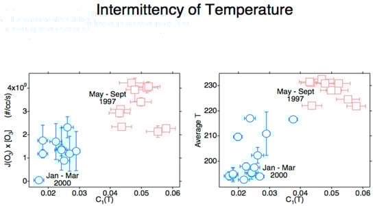
Figure 4.
Data from ER-2 observations during POLARIS [133,134] and SOLVE [137]. The abscissa in both diagrams is the intermittency of temperature. The ordinate in the left diagram is the ozone photodissociation rate averaged over the flight segment. The ordinate in the right diagram is the temperature averaged over the flight segment. Error bars are standard deviations. The correlations indicate incomplete thermalization of photofragment energy at 55 mbar.
Another consequential new observation was made in 1997, the WB57F Aerosol Mission (WAM). For the first time, the real-time analysis of individual aerosol particles was accomplished by the Particle Analysis by Laser Mass Spectrometry (PALMS). During six flights from Ellington Field (30° N, 95° W), over a million particles were encountered in the lower stratosphere and upper troposphere over the continental United States of America (USA) [138]. While sulfate-rich particles were predominant, pure ones were a rarity: 45 different elements were detected over the whole population between 5 and 19 km. Organics were abundant in the upper troposphere. They were even present in lesser amounts in the lowest 3–5 km of the stratosphere. The aerosol composition was more complex than previously appreciated, an important discovery given the role of accelerated chemistry in and on aerosols.
The high organic content of the tropospheric aerosols was incompatible with equilibrium constructs such as Henry’s Law and solubility. It was accountable by an inverted micelle model, with amphiphilic (organic surfactant) molecules forming an exterior film, with hydrophobic tails in the air and polar groups in the interior [139] exposed to the polar aqueous sulfurous core. This model was confirmed by Time-of-Flight Secondary Ion Mass Spectrometry (TOF-SIMS) on marine aerosols [140] and later on by continental samples [141].
The Stratospheric Tropospheric Experiment: Radiation, Aerosols and Ozone (STERAO) deployed aircraft, polarized Doppler radar and a three-dimensional radio interferometer to study the genesis of cumulonimbus storms on the Great Plains [142]. The location of the lightning strikes within the supercell was observed, and the NO production was measured in the outflow, combined with chemical measurements in the inflow. The event was successfully modeled numerically, giving confidence in the effect of a supercell on the connection between the troposphere and stratosphere.
In 1999, the Atmospheric Chemistry of Combustion Emissions Near the Tropopause (ACCENT) established a number of new observations that cast a fresh light on the composition of the upper tropical troposphere [143]. Two flights of the WB57F, from (30° N, 95° W) to (5° N, 95° W) on 19990920 and from (10° N, 86° W) to (30° N, 95° W) on 19990921 at a nominal altitude of 50,000’, equivalent to ≈15 km altitude, ≈360 K potential temperature and ≈125 mbar pressure. Ozone ranged between 3 and 130 parts per billion by volume (ppbv), with small-scale variability and varied correlations with a range of species having atmospheric lifetimes ranging from 10−2 to 103 years. Total water varied between 4 and 17 parts per million by volume (ppmv); the signature of molecules with a stratospheric sink indicated approximately 10% of the air along the flight tracks. The continuous, high-sensitivity methane observations showed the presence of stratospheric air between 12 and 17 km in the upper tropical troposphere [144].
The exhaust plumes from Delta II rockets, which used ammonium perchlorate (NH4ClO4/Al) oxidizer and liquid oxygen/kerosene fuel, were investigated by a stratospheric chemical payload carried on the WB57F at Cape Canaveral in 1998 [145]. The observed and modeled ozone losses in the promptly observed plumes were not in agreement, with the modeled loss falling short by about a factor of two on 720 s and 2340 s time scales at 18 and 18.6 km altitude. This result assumes greater importance in view of the rocket launch frequencies projected for later this century [146]—some as high as 15 per day—with the detritus from re-entry burnup of space vehicles being a potentially significant factor for climate as well as ozone loss.
Laboratory observations of water clusters [147] showed that absorption by the hydrogen-bonded water dimer was a significant factor in the near-infrared and visible transmissivity in the atmosphere [148]. Laboratory observations of overtone spectra of HNO3, HNO4 and H2O2 showed that photodissociation by near-infrared and visible wavelengths could produce free radicals, particularly at low zenith angles, i.e., at dawn and dusk and around the polar vortices in winter. The effect on pernitric acid, HNO4, solved a long-standing problem of NOy speciation throughout the lower stratosphere [149,150]. Further laboratory work revealed a similar photodissociation of sulfuric acid, H2SO4, yielding a source of sulfur dioxide, SO2, in the stratosphere [151].
In the Arctic winter of 1999–2000, a large mission involving several countries was mounted to further explore the stratospheric vortex’s chemistry and dynamics, the SAGE-III Ozone Loss and Validation Experiment/Third European Stratospheric Experiment (SOLVE/THESEO) [137]. Much of the airborne focus centered on Kiruna (67° N, 20° E), but there were balloon profiles elsewhere, with satellite observations and general circulation modeling providing a global context.
An important observation was the formation of large nitric acid–water particles at temperatures above the frost point, enabling denitrification without cooling to temperatures where dehydration could occur [152]. The ozone loss so enabled reached an estimated 58% at about 20 km altitude, a loss rate of 46 ppbv/day in the inner vortex [153]. That calculation ignored the diluting contribution of dynamical mixing within the inner vortex defined as bounded by a measured wind speed of 30 ms−1. Including it via a scaling analysis had the photochemical ozone loss rate within the inner vortex, as defined by the measured wind speed definition, proceeding at 17–33 ppbv/day [154] or about half the rate calculated excluding dynamics.
A further application of statistical multifractal analysis showed that the calculation of chemical loss rates in a turbulent medium of 23/9 dimensions necessitated changes in the application of the law of mass action [155].
Combining observations in the tropics and subtropics by the ER-2 and WB57F resulted in conclusions that the subtropical jet stream was a site of exchange between the upper tropical troposphere and the lower midlatitude stratosphere and that the tropopause between the subtropical jet stream and the inner tropics at 95oW sloped downwards from a potential temperature θ ≈ 400 K at 30° N to ≈380 K at 10° N [11]. The tropical surface moist static energy θw maximizes at 355 K, showing that the transport of higher θ air from the subtropical stratosphere is involved in determining the tropical tropopause.
The CRYSTAL-FACE (Cirrus Regional Study of Tropical Anvils and Cirrus Layers—Florida Area Cirrus Experiment) mission from Key West (25° N, 82° W) in 2002 detected deep penetration of tracked North American forest fire plumes up to potential temperatures of 393 K, 15.8 km and 1.7 km above the local tropopause [156]. Comprehensive chemical and aerosol signatures were available from the WB57F payload.
The pre-AVE (Aura Validation Experiment) mission from San José (10° N, 84° W) featured flights of the WB57F both north and south in the lower stratosphere and profiles above the airbase from the surface to 18 km altitude. Accurate, high-precision measurements of CH4 established the presence of stratospheric air between 12 km and the tropopause at 17 km and enabled the examination of four stages in the dehydration of the air in the tropical stratosphere. A detailed mechanism was proposed that entailed evaporative distillation of small ice particles onto larger ones with a significant fall velocity [157]. The single aerosol particle measurements [138] were combined with later observations to offer a comprehensive review of aerosol properties [158].
Analysis of aerosol composition at the surface in Scandinavia showed that fatty acids up to C32 molecules were on continental aerosols [141]. Some of these could be transported to the lower stratosphere, by cumulonimbus, pyrocumulus and during cyclogenesis.
The NOAA Winter Storms project, held over the eastern Pacific Ocean during the January–March winters of 2004, 2005 and 2006 deployed the G4 aircraft to drop a total of 885 GPS dropsondes from about 13 km in an area bounded by 15° N–60° N, 128° W–172° W [159]. The scaling characteristics of the winds, temperatures and humidity were established and found for horizontal wind speed to increase from the boundary layer to jet streams at up to 12.8 km. Isotropy was never observed [160]. Analysis of ozone data revealed the transport of midlatitude lower stratospheric ozone into the tropical marine boundary layer and to the subtropical anticyclone’s cloud decks [161].
Later analysis of WAM data showed activation of chlorine in the vicinity of the midlatitude tropopause, consistent with water content, aerosol amounts and a mechanism involving heterogeneous chemistry at temperatures above the frost point. The water mixing ratio was in the range of 20–25 ppm [162]; the water content of aerosols is a vital factor in their generation and chemical activity [126,163,164].
With respect to the definition of the tropopause, analysis of GPS dropsonde data from the NOAA G4 [159,160] showed that at vertical scales below 30m, the air immediately above and below the tropopause was indistinguishable as stratospheric or tropospheric, as shown in Figure 5.
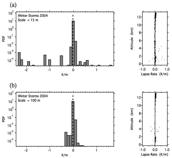
Figure 5.
Change in temperature with altitude (the lapse rate). The dry adiabatic lapse rate (DALR) is 9.8 K/km and is marked by the vertical dashed line. The data are from Winter Storms 2004 [159,160] and were calculated for (a) a vertical interval of 15 m and (b) a vertical interval of 100 m. In (a), about 1% of the cases exceed the dry adiabatic lapse rate, whereas in (b), none do. The tropopause is discernible at vertical resolutions above 30 m using this criterion, but not below it. The 50% exceedance of the DALR is, by extrapolation, at 93 cm. Note that fluid flow emerges from a simulated molecular dynamics population of Maxwellian billiards in an asymmetric environment on very short time and space scales [165,166].
5. WMO Reports and Assessments of Stratospheric Ozone
The World Meteorological Organization (WMO) has produced a series of documents beginning in 1981 that reviewed the then-current state of research into stratospheric ozone, starting with WMO Report No. 11 and most recently with No. 1268 in 2021. The Montreal Protocol and its Amendments formalized and accelerated the production of Assessments beginning in 1989, and there have been a further nine, at 4-year intervals, since 1994. The most recent chronicles the series and offers the current assessment [167]. It is evident that the series is necessary because the increased scope and accelerated pace of research have led to continued discoveries following experimental results, observations and model improvements. Examples are the results from lower stratospheric airborne observations of water and ozone [2,3,4,90]; reactive nitrogen [29,38,58,73,91,92,98] and reactive and total chlorine [40,43,44,52,94,95,99]. There are many others in the references covering eight decades. The discoveries include dynamical mechanisms, radiative transfer processes and chemical measurements of reactive species such as HOx. The process of observing variables and understanding their nonlinear interactions is still incomplete [167]. The entanglement of the ozone loss problem with climate change generally has been a growing theme, particularly since the hydrofluorocarbons (HFCs) that are replacing the chlorofluorocarbons (CFCs) are infrared active. Both species are “greenhouse” gases, infrared active and affect the climate. Because the H atom is readily attacked by the tropospheric OH, the HFCs do not get above the bottom scale height (approximately 7 km) of the stratosphere (Figure 1) but do have significant effects from there, see Chapters 2 and 5 of [167]. This current report has considered geoengineering [168,169,170], particularly in the form of Stratospheric Aerosol Injection (SAI), previously known as solar radiation management, as stated in its Chapter 6. Other methods proposed are Marine Cloud Brightening (MCB) and Cirrus Cloud Thinning (CCT). Geoengineering is a proposed deliberate intervention by injecting aerosols into the lower stratosphere that will cool the surface by scattering and absorbing solar radiation at the expense of locally heating the lower stratosphere. MCB is posited to reflect more solar radiation to space by encouraging more cloud formation by the induction of more nucleating particles. CCT acts to thin high-altitude cirrus, which is believed to reduce outgoing infrared radiation to space. All three methods depend upon the injection or production of manageable quantities of aerosols at sensitive sites in the atmosphere, with the objective of countering the heating of the surface atmosphere by fossil fuel burning, methane, nitrous oxide, CFCs, HCFCs and the water vapour from positive feedback. The logistics will not be trivial [170] but are of magnitudes that look possible, at least in principle.
6. Forecasts: Macroweather and Climate
The ability to forecast the future evolution of the lower stratosphere and the associated jet streams is tied to the ability to forecast the underlying tropospheric evolution [11,167,171,172,173,174]. That will in turn involve stochastic approaches and reductions to grid size to improve efforts much beyond 10 days. A horizontal resolution of 1 km has been proposed as necessary, but it is an unproven proposition. Both approaches will require extensive development and testing, with uncertain outcomes. Scaling analysis points to the absence of local thermodynamic equilibrium and the need to address questions about the representation of the wind speeds observed in jet streams, hurricanes and tornadoes [160,165,175].
Current climate models are argued not to predict climate, but macroweather, the meteorological regime that spans 10 days to 20 years [172]. That of course has utility but comes with large sensitivity to initial conditions, a constraint that will apply irrespective of spatial resolution. Further relevant work can be found in [173,174].
An important feature of the statistical multifractal analysis is that variances do not converge, in this case for winds, temperature, total water, ozone and nitrous oxide [175]. See reference [174] for a detailed review. The non-convergence of variance is illustrated in a larger context in [41] (Figure Q13-1), a clear demonstration that smooth or compact inputs to the coupled, nonlinear system of the atmosphere result in large variations in observed variables, with consequences for predictability.
7. Discussion and Conclusions
What we see in the progression of knowledge during the last seven decades is that original, accurate experiments and observations result in significant consequences for understanding and ability to simulate the stratosphere and its ozone content. The current state of knowledge [41,167] makes it clear that even in the present advanced stage, uncertainties persist. Here, we point out some associated with geoengineering [170].
With regard to the three types of geoengineering, SAI, MCB and CCT, we note that the venues of these interventions are interactively connected by the dynamics observed in [161]. Furthermore, the supply of total water will be central to the chemistry and cloud physics in all three venues and on all scales from molecular to global [4,10,11,66,67,90,131,143,148,156,164,176,177,178,179,180]. The current ability of climate models to reproduce the distribution of relative humidity is less than adequate over continental North America, for example [176]. The reliance on the Mt. Pinatubo eruption for a “calibration” of SAI may have significant uncertainties [177]. The variability in the response to a pulsed input is consistent with the non-convergence of variance, leaving the way open for differing interpretations of the uncertainties.
Examples of recent publications, among many, that have significant implications for the state of the lower stratosphere are [178,179,180]. The water content is, once again, central. It seems likely that since the Hunga Tonga eruption raised about 500 m of ocean into the stratosphere, there would have been organic molecular content injected into the stratosphere, which is a potential complication. With many particles containing transition metals in the stratospheric aerosol, chemical uncertainties abound—they are well-known as catalysts in chemistry. Iron, nickel and copper, for example, heterogeneously catalyze the production of ammonia, the hydration of vegetable oils and the oxidation of alcohols, respectively; these are a few examples among many. The metals already found in aerosol particles in the lower stratosphere conclusively indicate the presence of materials from rocket launches and the eventual burnup of their payloads upon re-entry to the atmosphere [178]. Some projections of the frequency of commercial launches run as high as 15 per day.
Air entering the bottom scale height of the stratosphere enters, with its chemical burden, from several directions including downward descent from the mesosphere and upper stratosphere in the winter vortices and their surroundings; upward entry from tropospherically based cumulonimbus storms and pyrocumulus clouds and horizontally by exchange across both subtropical and polar front jet streams and the associated tropopauses. It leaves by tropopause folding around jet streams into the upper troposphere, by small-scale turbulence and by radiative subsidence. These processes interact nonlinearly and are characterized by variances that do not converge. There is much left to do before confident, quantitative prediction is achieved.
The complexities of the interactions between radiative, chemical and dynamical processes on all scales have considerable implications for their reliable calculation, and hence, for policy decisions. The more reliable approach is to lean on analysis of observations [173,174], whether considering ozone depletion, global heating or air pollution.
These considerations have implications for future research. There is no substitute for high-quality, well-thought-out experimental work in laboratories and in the field that addresses the issues on all scales, from molecular through meteorological to global, and which pose critical tests for modeling.
Funding
This research received no external funding.
Institutional Review Board Statement
Not applicable.
Informed Consent Statement
Not applicable.
Data Availability Statement
Data used are available on the NASA Airborne Database https://earthdata.nasa.gov/esds/impact/admg/the airborne-inventory (accessed on 5 June 2021).
Conflicts of Interest
The author declares no conflict of interest.
References
- Dobson, G.M.B.; Brewer, A.W.; Cwilong, B.M. Meteorology of the lower stratosphere. Proc. R. Soc. A 1945, 185, 144–175. [Google Scholar]
- Brewer, A.W.; Cwilong, B.M.; Dobson, G.M.B. Measurement of absolute humidity in very dry air. Proc. Phys. Soc. 1948, 60, 52–70. [Google Scholar] [CrossRef]
- Brewer, A.W. Evidence for a world circulation provided by measurements of the helium and water vapour distributions in the stratosphere. Q. J. R. Meteorol. Soc. 1949, 75, 351–363. [Google Scholar] [CrossRef]
- Foot, J.S. Aircraft measurements of the humidity in the lower stratosphere from 1977 to 1980 between 45° N and 65° N. Q. J. R. Meteorol. Soc. 1984, 110, 303–319. [Google Scholar]
- Tuck, A.F.; Browell, E.V.; Danielsen, E.F.; Holton, J.R.; Hoskins, B.J.; Johnson, D.R.; Kley, D.; Krueger, A.J.; Mégie, G.; Newell, R.E.; et al. Stratosphere-Troposphere Exchange. In Atmospheric Ozone 1985; World Meteorological Organization: Geneva, Switzerland, 1986; Chapter 5. [Google Scholar]
- Mattingly, S.R. The contribution of extratropical severe storms to the stratospheric water vapour budget. Meteorol. Mag. 1977, 106, 256–262. [Google Scholar]
- Sawyer, J.S. The dynamical systems of the lower stratosphere. Q. J. R. Meteorol. Soc. 1951, 77, 480–483. [Google Scholar] [CrossRef]
- Reed, R.J.; Danielsen, E.F. Fronts in the vicinity of the tropopause. Arch. Meteorol. Geophys. Bioklim. 1959, 11, 1–17. [Google Scholar] [CrossRef]
- Briggs, J.; Roach, W.T. Aircraft observations near jet streams. Q. J. R. Meteorol. Soc. 1963, 89, 225–247. [Google Scholar] [CrossRef]
- Tuck, A.F.; Baumgardner, D.; Chan, K.R.; Dye, J.E.; Elkins, J.W.; Hovde, S.J.; Kelly, K.K.; Loewenstein, M.; Margitan, J.J.; May, R.D.; et al. The Brewer-Dobson circulation in the light of high altitude in situ aircraft observations. Q. J. R. Meteorol. Soc. 1997, 123, 1–69. [Google Scholar]
- Tuck, A.F.; Hovde, S.J.; Kelly, K.K.; Mahoney, M.J.; Proffitt, M.H.; Richard, E.C.; Thompson, T.L. Exchange between the upper tropical troposphere and the lower stratosphere studied with aircraft observations. J. Geophys. Res. 2003, 108, 4734. [Google Scholar] [CrossRef]
- Murgatroyd, R.J.; Clews, C.J.B. Wind at 100,000 ft. over South-East England. In Meteorological Office Geophysical Memoirs; HMSO: London, UK, 1949; p. 83. [Google Scholar]
- Murgatroyd, R.J. Winds and temperatures between 20 km and 100 km—A review. Q. J. R. Meteorol. Soc. 1957, 83, 417–458. [Google Scholar] [CrossRef]
- Pittock, A.B. A thin stable layer of anomalous ozone and dust content. J. Atmos. Sci. 1966, 23, 538–542. [Google Scholar] [CrossRef][Green Version]
- Dyer, A.J.; Hicks, B.B. Global spread of volcanic dust from the Bali eruption of 1963. Q. J. R. Meteorol. Soc. 1968, 94, 545–554. [Google Scholar] [CrossRef]
- Newell, R.E. Stratospheric temperature change from the Mt. Agung volcanic eruption of 1963. J. Atmos. Sci. 1970, 27, 977–978. [Google Scholar] [CrossRef]
- Junge, C.E. Air Chemistry and Radioactivity; Academic Press: New York, NY, USA, 1963. [Google Scholar]
- Brode, H.L. Review of nuclear weapon effects. Ann. Rev. Nucl. Sci. 1960, 18, 153–202. [Google Scholar] [CrossRef]
- Reid, S.J.; Tuck, A.F.; Kiladis, G. On the changing abundance of ozone minima at northern midlatitudes. J. Geophys. Res. 2000, 105, 12169–12180. [Google Scholar] [CrossRef]
- Müller, R. A brief history of stratospheric ozone research. Meteorol. Zeitschift 2009, 1, 3–24. [Google Scholar] [CrossRef]
- Chapman, S. A theory of upper atmospheric ozone. Mem. R. Meteorol. Soc. 1930, 3, 103–109. [Google Scholar]
- Brewer, A.W.; Wilson, A.W. The regions of formation of atmospheric ozone. Q. J. R. Meteorol. Soc. 1968, 94, 249–265. [Google Scholar] [CrossRef]
- Bates, D.R.; Nicolet, M. The photochemistry of atmospheric water vapour. J. Geophys Res. 1950, 55, 301–327. [Google Scholar] [CrossRef]
- Hunt, B.G. Photochemistry of ozone in a moist atmosphere. J. Geophys. Res. 1966, 71, 1385–1398. [Google Scholar] [CrossRef]
- Hampson, J. Photochemical Behaviour of the Ozone Layer; Technical Note 1627; Canadian Armament and Research Establishment: Valcartier, QC, Canada, 1964; pp. 1–280. [Google Scholar]
- Hampson, J. Chemiluminescent emissions observed in the stratosphere and mesosphere. In Les Problèmes Météorologiques de la Stratosphère et de la Mésosphère; Nicolet, M., Ed.; Centre National d’Études Spatiales: Paris, France, 1965. [Google Scholar]
- Hampson, J. Atmospheric Energy Change by Pollution of the Upper Atmosphere; CARDE Technical Note 1738; Canadian Armament Research and Development Establishment: Valcartier, QC, Canada, 1966. [Google Scholar]
- Crutzen, P.J. The influence of nitrogen oxides on the atmospheric ozone content. Q. J. R. Meteorol. Soc. 1970, 96, 320–325. [Google Scholar] [CrossRef]
- Murcray, D.G.; Kyle, T.G.; Murcray, F.H.; Williams, W.J. Nitric acid and nitric oxide in the lower stratosphere. Nature 1968, 218, 78–79. [Google Scholar] [CrossRef]
- Goody, R.M.; Walker, J.C.G. Atmospheres; Prentice Hall Inc.: Englewood Cliffs, NK, USA, 1972. [Google Scholar]
- Johnston, H. Reduction of stratospheric ozone by nitrogen oxide catalysts from supersonic transport exhaust. Science 1971, 173, 517–522. [Google Scholar] [CrossRef]
- Crutzen, P.J. Ozone production rates in an oxygen-hydrogen-nitrogen oxide atmosphere. J. Geophys. Res. 1971, 76, 7311–7333. [Google Scholar] [CrossRef]
- Zel’dovich, Y.B.; Raizer, Y.P. Physics of Shock Waves and High-Temperature Hydrodynamic Phenomena; Dover: Minola, NY, USA, 2002. [Google Scholar]
- Goldsmith, P.; Tuck, A.F.; Foot, J.S.; Simmons, E.L.; Newson, R.L. Nitrogen oxides, nuclear weapon testing, Concorde and stratospheric ozone. Nature 1973, 244, 545–551. [Google Scholar] [CrossRef]
- Tuck, A.F. Production of nitrogen oxides by lightning discharges. Q. J. R. Meteorol. Soc. 1976, 102, 749–755. [Google Scholar] [CrossRef]
- Brune, W.H.; McFarland, P.J.; Bruning, E.; Waugh, S.; McGorman, D.; Miller, D.O.; Jenkins, M.J.; Ren, X.; Mao, J.; Peischl, J. Extreme oxidant amounts produced by lightning in storm clouds. Science 2021, 372, 711–715. [Google Scholar] [CrossRef]
- Wang, H.; Pei, Y.; Yin, Y.; Shen, L.; Chen, K.; Shi, Z.; Chen, J. Observational evidence of lightning-generated ultrafine aerosols. Geophys. Res. Lett. 2021, 48, e2021GL093771. [Google Scholar] [CrossRef]
- Fahey, D.W.; Keim, E.R.; Boering, K.A.; Brock, C.A.; Wilson, J.C.; Jonsson, H.H.; Anthony, S.; Hanisco, T.F.; Wennberg, P.O.; Miake-Lye, R.C. Emission measurements of the Concorde supersonic aircraft in the lower stratosphere. Science 1995, 270, 70–74. [Google Scholar] [CrossRef]
- Molina, M.J.; Rowlad, F.S. Stratospheric sink for chlorofluoromethanes—Chlorine atom catalyzed destruction of ozone. Nature 1974, 249, 810–812. [Google Scholar] [CrossRef]
- Lovelock, J.E.; Maggs, R.J.; Wade, R.J. Halogenated hydrocarbons in and over the Atlantic. Nature 1973, 241, 194–196. [Google Scholar] [CrossRef]
- Salawitch, R.J.; McBride, L.A.; Thompson, C.R.; Fleming, E.L.; McKenzie, R.L.; Rosenlof, K.H.; Doherty, S.J.; Fahey, D.W. Twenty Questions and Answers about the Ozone Layer: 2022 Update; World Meteorological Organization: Geneva, Switzerland, 2023; 75p. [Google Scholar]
- Groves, K.S.; Tuck, A.F. Stratospheric O3-CO2 coupling in a photochemical-radiative column model. II. With chlorine chemistry. Q. J. R. Meteorol. Soc. 1980, 106, 141–157. [Google Scholar] [CrossRef]
- Anderson, J.G.; Margitan, J.J.; Stedman, D.H. Atomic chlorine and the chlorine monoxide radical in the stratosphere: Three in situ observations. Science 1977, 198, 501–503. [Google Scholar] [CrossRef]
- Farmer, C.B.; Raper, O.F.; Norton, R.H. Spectroscopic detection and vertical distribution of HCl in the troposphere and stratosphere. Geophys. Res. Lett. 1976, 3, 13–16. [Google Scholar] [CrossRef]
- Ackerman, M.; Frimout, D.; Girard, A.; Gottignies, M.; Muller, C. Stratospheric HCl from infrared spectra. Geophys. Res. Lett. 1976, 3, 81–83. [Google Scholar] [CrossRef]
- Williams, W.J.; Kosters, J.J.; Goldman, A.; Murcray, D.G. Measurement of the stratospheric mixing ratio of HCl using infrared absorption technique. Geophys. Res. Lett. 1976, 3, 383–385. [Google Scholar] [CrossRef]
- Eyre, J.R.; Roscoe, H.K. Radiometric measurement of stratospheric HCl. Nature 1977, 266, 243–244. [Google Scholar] [CrossRef]
- Lazrus, A.L.; Gandrud, B.W.; Woodward, E.N.; Sedlacek, W.A. Direct measurements of of stratospheric chlorine and bromine. J. Geophys. Res. 1976, 81, 1067–1070. [Google Scholar] [CrossRef]
- Clyne, M.A.A.; Watson, R.T. Kinetic studies for diatomic free radicals using mass spectrometry. Part 3.—Elementary reactions involving BrO X2Π radicals. J. Chem. Soc. Farad. Trans. 1 1975, 71, 336–350. [Google Scholar] [CrossRef]
- Shaw, J.H.; Sutherland, G.B.B.M.; Wormell, T.W. Nitrous oxide in the Earth’s atmosphere. Phys. Rev. 1948, 74, 978–979. [Google Scholar]
- Williamson, E.J.; Houghton, J.T. Radiometric measurements of emission from stratospheric water vapour. Q. J. R. Meteorol. Soc. 1965, 91, 330–338. [Google Scholar] [CrossRef]
- Schmeltekopf, A.L.; Goldan, P.D.; Henderson, W.R.; Harrop, W.J.; Thompson, T.L.; Fehsenfeld, F.C.; Schiff, H.I.; Crutzen, P.J.; Isaksen, I.S.A.; Ferguson, E.E. Measurements of stratospheric CFCl3, CF2Cl2 and N2O. Geophys. Res. Lett. 1975, 2, 393–396. [Google Scholar] [CrossRef]
- Goldan, P.D.; Kuster, W.C.; Albritton, D.L.; Schmeltekopf, A.L. Stratospheric CFCl3, CF2Cl2, and N2O height profile measurements at several latitudes. J. Geophys. Res. Atmos. 1979, 85, 413–423. [Google Scholar] [CrossRef]
- Delwiche, C.C. Biological production and utilization of N2O. Pure Appl. Geophys. 1978, 116, 414–422. [Google Scholar] [CrossRef]
- Rowland, F.S.; Spencer, J.E.; Molina, M.J. Stratospheric formation and photolysis of chlorine nitrate. J. Phys. Chem. 1976, 80, 2711–2713. [Google Scholar] [CrossRef]
- Cox, R.A.; Derwent, R.G.; Eggleton, A.E.J. Chlorine Nitrate—A Possible Stratospheric Sink for ClO Radicals and NOx with Significant Implications for Ozone Depletion; Atomic Energy Research Establishment Report 8383; AERE: Harwell, UK, 1976. [Google Scholar]
- Brasseur, G.P.; Solomon, S. Aeronomy of the Middle Atmosphere, 3rd ed.; Springer: Dordrecht, The Netherlands, 2005. [Google Scholar]
- Harries, J.E. Measurements of some hydrogen-oxygen-nitrogen compounds in the stratosphere from Concorde 002. Nature 1973, 241, 515–518. [Google Scholar] [CrossRef]
- Harries, J.E.; Moss, D.G.; Swann, N.R.W.; Neill, G.F.; Gildwarg, P. Simultaneous measurements of H2O, NO2 and HNO3 in the daytime stratosphere from 15 to 35 km. Nature 1976, 259, 300–302. [Google Scholar] [CrossRef]
- Harries, J.E. Ratio of HNO3 to NO2 concentrations in daytime stratosphere. Nature 1978, 274, 235. [Google Scholar] [CrossRef]
- Anderson, J.G. Odd chlorine processes. In Stratospheric Ozone and Man; CRC Press: Boca Raton, FL, USA, 1982; Chapter 6. [Google Scholar]
- McCormick, M.P.; Hamill, P.; Pepin, T.J.; Chu, W.P.; Swissler, T.J.; McMaster, L.R. Satellite studies of the stratospheric aerosol. Bull. Am. Meteorol. Soc. 1979, 60, 1038–1046. [Google Scholar] [CrossRef]
- McCormick, M.P.; Steele, H.M.; Hamill, P.; Chu, W.P.; Swissler, T.J. Polar stratospheric cloud sightings by SAM II. J. Atmos. Sci. 1982, 40, 1387–1397. [Google Scholar] [CrossRef]
- Murgatroyd, R.J. Recent progress in studies of the stratosphere. Q. J. R. Meteorol. Soc. 1982, 108, 271–312. [Google Scholar] [CrossRef]
- Fels, S.B.; Mahlman, J.D.; Schwarzkopf, M.D.; Sinclair, R.W. Stratospheric sensitivity to perturbations in ozone and carbon dioxide: Radiative and dynamical response. J. Atmos. Sci. 1980, 38, 2265–2297. [Google Scholar] [CrossRef]
- Allam, R.J.; Tuck, A.F. Transport of water vapour in a stratosphere-troposphere general circulation model. I: Fluxes. Q. J. R. Meteorol. Soc. 1984, 110, 321–356. [Google Scholar] [CrossRef]
- Allam, R.J.; Tuck, A.F. Transport of water vapour in a stratosphere-troposphere general circulation model. II: Trajectories. Q. J. R. Meteorol. Soc. 1984, 357–392. [Google Scholar] [CrossRef]
- O’Neill, A. The dynamics of stratospheric warmings generated by a general circulation model of the troposphere and stratosphere. Q. J. R. Meteorol. Soc. 1980, 106, 659–690. [Google Scholar] [CrossRef]
- O’Neill, A.; Newson, R.L.; Murgatroyd, R.J. An analysis of the large-scale features of the upper troposphere and the stratosphere in a global, three-dimensional general circulation model. Q. J. R. Meteorol. Soc. 1982, 108, 25–53. [Google Scholar] [CrossRef]
- Newell, R.E.; Gould-Stewart, S. A stratospheric fountain? J. Atmos. Sci. 1981, 38, 2789–2796. [Google Scholar] [CrossRef]
- Robinson, G.D. The transport of minor atmospheric constituents between troposphere and stratosphere. Q. J. R. Meteorol. Soc. 1980, 106, 227–253. [Google Scholar] [CrossRef]
- Bamber, D.J.; Healey, P.G.W.; Jones, B.M.R.; Penkett, S.A.; Tuck, A.F.; Vaughan, G. Vertical profiles of tropospheric gases: Chemical consequences of stratospheric intrusions. Atmos. Environ. 1984, 18, 1759–1766. [Google Scholar] [CrossRef]
- Noxon, J.F. Stratospheric NO2 in the Antarctic winter. Geophys. Res. Lett. 1978, 5, 1021–1022. [Google Scholar] [CrossRef]
- Noxon, J.F. Stratospheric NO2, 2. Global behavior. J. Geophys. Res. 1984, 84, 5067–5076. [Google Scholar] [CrossRef]
- Farman, J.C.; Murgatroyd, R.J.; Silnickas, A.M.; Thrush, B.A. Ozone photochemistry in the Antarctic stratosphere in summer. Q. J. R. Meteorol. Soc. 1985, 111, 1013–1025. [Google Scholar] [CrossRef]
- Farman, J.C.; Gardiner, B.G.; Shanklin, J.D. Large losses of total ozone in the Antarctica reveal seasonal ClOx/NOx interaction. Nature 1985, 315, 207–210. [Google Scholar] [CrossRef]
- Stolarski, R.S.; Krueger, A.J.; Schoeberl, M.R.; McPeters, R.D.; Newman, P.A.; Alpert, J.C. Nimbus 7 satellite measurements of the springtime Antarctic ozone decrease. Nature 1986, 332, 808–811. [Google Scholar] [CrossRef]
- Solomon, S.; Garcia, R.R.; Rowland, F.S.; Wuebbles, D.J. On the depletion of Antarctic ozone. Nature 1986, 321, 755–758. [Google Scholar] [CrossRef]
- Hayman, G.D.; Davies, J.M.; Cox, R.A. Kinetics of the reaction ClO + ClO → products and its potential relevance to Antarctic ozone. Geophys. Res. Lett. 1986, 13, 1347–1350. [Google Scholar] [CrossRef]
- Molina, L.T.; Molina, M.J. Production of Cl2O2 from the self reaction of the ClO radical. J. Phys. Chem. 1987, 91, 433–436. [Google Scholar] [CrossRef]
- Austin, J.; Garcia, R.R.; Russell, J.M., III; Solomon, S.; Tuck, A.F. On the atmospheric photochemistry of nitric acid. J. Geophys. Res. 1986, 91, 5477–5485. [Google Scholar] [CrossRef]
- Austin, J.; Remsberg, E.E.; Jones, R.L.; Tuck, A.F. Polar Stratospheric Clouds inferred for satellite data. Geophys. Res. Lett. 1986, 13, 1256–1259. [Google Scholar] [CrossRef]
- Hanson, D.; Mauersberger, K. Laboratory studies of the nitric acid hydrate: Implications for the south polar stratosphere. Geophys. Res. Lett. 1988, 15, 855–858. [Google Scholar] [CrossRef]
- Mount, G.H.; Sanders, R.W.; Schmeltekopf, A.L.; Solomon, S. Visible spectroscopy at McMurdo station, Antarctica, 1. Overview and daily variations of NO2 and O3 during austral spring, 1986. J. Geophys. Res. 1987, 92, 8320–8328. [Google Scholar] [CrossRef]
- Solomon, S.; Mount, G.H.; Sanders, R.W.; Schmeltekopf, A.L. Visible spectroscopy at McMurdo station, Antarctica, 2. Observations of OClO. J. Geophys. Res. 1987, 92, 8329–8338. [Google Scholar] [CrossRef]
- Farmer, C.B.; Toon, G.C.; Shaper, P.W.; Blavier, J.F.; Lowes, L.L. Ground-based measurements of the composition of the Antarctic atmosphere during the 1986 spring season, I, Stratospheric trace gases. Nature 1987, 329, 126–130. [Google Scholar] [CrossRef]
- Hofmann, D.J.; Harder, J.W.; Rolf, S.R.; Rosen, J.M. Balloon-borne observations of the temporal development and vertical structure of the Antarctic ozone hole in 1986. Nature 1987, 326, 59–62. [Google Scholar] [CrossRef]
- Komhyr, W.D.; Grass, R.D.; Reitelbach, P.J.; Kuester, S.E.; Franchois, P.R.; Fanning, M.L. Total ozone, ozone vertical distributions, and stratospheric temperatures at South Pole, Antarctica in 1986 and 1987. J. Geophys. Res. 1989, 94, 11429–11436. [Google Scholar] [CrossRef]
- Tuck, A.F.; Watson, R.T.; Condon, E.P.; Margitan, J.J.; Toon, O.B. The planning and execution of ER-2 and DC-8 aircraft flights over Antarctica, August and September 1987. J. Geophys. Res. 1989, 94, 11181–11222. [Google Scholar] [CrossRef]
- Kelly, K.K.; Tuck, A.F.; Murphy, D.M.; Proffitt, M.H.; Fahey, D.W.; Jones, R.L.; McKenna, D.S.; Loewenstein, M.; Podolske, J.R.; Strahan, S.E.; et al. Dehydration in the lower Antarctic stratosphere during late winter and early spring, 1987. J. Geophys. Res. 1989, 94, 11317–11358. [Google Scholar] [CrossRef]
- Fahey, D.W.; Kelly, K.K.; Ferry, G.V.; Poole, L.R.; Wilson, J.C.; Murphy, D.M.; Loewenstein, M.; Chan, K.R. In situ measurements of total reactive nitrogen, total water, and aerosol in a polar stratospheric cloud in the Antarctic. J. Geophys. Res. 1989, 94, 11299–11316. [Google Scholar] [CrossRef]
- Fahey, D.W.; Murphy, D.M.; Kelly, K.K.; Ko, M.K.W.; Proffitt, M.H.; Eubank, C.S.; Ferry, G.V.; Loewenstein, M.; Chan, K.R. Measurements of nitric oxide and total reactive nitrogen in the Antarctic stratosphere: Observations and chemical implications. J. Geophys. Res. 1989, 94, 16665–16682. [Google Scholar] [CrossRef]
- Anderson, J.G.; Brune, W.H.; Proffitt, M.H. Ozone destruction by chlorine radicals within the Antarctic vortex: The spatial and temporal evolution of ClO-O3 anticorrelation based on in situ ER-2 data. J. Geophys. Res. 1989, 94, 11465–11480. [Google Scholar] [CrossRef]
- Brune, W.H.; Anderson, J.G.; Chan, K.R. In situ observations of BrO over Antarctica: ER-2 aircraft results from 54° S to 72° S latitude. J. Geophys. Res. 1989, 94, 16639–16648. [Google Scholar] [CrossRef]
- Brune, W.H.; Anderson, J.G.; Chan, K.R. In situ observations of ClO in the Antarctic: ER-2 aircraft results from 54° S to 72° S latitude. J. Geophys. Res. 1989, 94, 16649–16664. [Google Scholar] [CrossRef]
- Proffitt, M.H.; Powell, J.A.; Tuck, A.F.; Fahey, D.W.; Kelly, K.K.; Krueger, A.J.; Schoeberl, M.R.; Gary, B.L.; Margitan, J.J.; Chan, K.R.; et al. A chemical definition of the boundary of the Antarctic ozone hole. J. Geophys. Res. 1989, 94, 11437–11448. [Google Scholar] [CrossRef]
- Proffitt, M.H.; Steinkamp, M.J.; Powell, J.A.; McLaughlin, R.J.; Mills, O.A.; Schmeltekopf, A.L.; Thompson, T.L.; Tuck, A.F.; Tyler, T.; Winkler, R.H.; et al. In-situ measurements within the 1987 Antarctic ozone hole from a high-altitude ER-2 aircraft. J. Geophys. Res. 1989, 94, 16547–16556. [Google Scholar] [CrossRef]
- Loewenstein, M.; Podolske, J.R.; Chan, K.R.; Strahan, S.E. Nitrous oxide as a dynamical tracer in the 1987 Airborne Antarctic Ozone Experiment. J. Geophys. Res 1989, 94, 11589–11598. [Google Scholar] [CrossRef]
- Heidt, L.E.; Vedder, J.F.; Pollock, W.H.; Lueb, R.A.; Henry, B.A. Trace gases in the Antarctic atmosphere. J. Geophys. Res. 1989, 94, 11599–11612. [Google Scholar] [CrossRef]
- Tuck, A.F. Synoptic and chemical evolution in the Antarctic vortex in late winter and early spring, 1987. J. Geophys. Res. 1989, 94, 11687–11737, Erratum in J. Geophys. Res. 1989, 94, 16855. [Google Scholar] [CrossRef]
- Turco, R.P.; Plumb, R.A.; Condon, E. The Airborne Arctic Stratospheric Expedition: Prologue. Geophys. Res. Lett. 1990, 17, 313–316. [Google Scholar] [CrossRef]
- Brune, W.H.; Toohey, D.W.; Anderson, J.G.; Chan, K.R. In situ observations of ClO in the Arctic stratosphere: ER-2 aircraft results from 59° N to 80° N latitude. Geophys. Res. Lett. 1990, 17, 505–508. [Google Scholar] [CrossRef]
- Hübler, G.; Fahey, D.W.; Kelly, K.K.; Montzka, D.D.; Carroll, M.A.; Tuck, A.F.; Heidt, L.E.; Pollock, W.H.; Gregory, G.L.; Vedder, J.F. Redistribution of reactive odd nitrogen in the lower Arctic stratosphere. Geophys. Res. Lett 1990, 17, 453–456. [Google Scholar] [CrossRef]
- Dye, J.E.; Baumgardner, D.; Gandrud, B.W.; Kawa, S.R.; Kelly, K.K.; Loewenstein, M.; Ferry, G.V.; Chan, K.R.; Gary, B.L. Particle size distribution in Arctic polar stratospheric clouds, growth and freezing of sulfuric acid droplets, and implications for ice cloud formation. J. Geophys. Res. 1992, 97, 8015–8034. [Google Scholar] [CrossRef]
- Browell, E.V.; Butler, C.F.; Ismail, S.; Robinette, P.A.; Carter, A.F.; Higdon, N.S.; Toon, O.B.; Schoeberl, M.R.; Tuck, A.F. Airborne lidar observations in the wintertime Arctic stratosphere: Polar stratospheric clouds. Geophys. Res. Lett. 1990, 17, 325–328. [Google Scholar] [CrossRef]
- Jones, R.L.; McKenna, D.S.; Poole, L.R.; Solomon, S. On the influence of polar stratospheric cloud formation on chemical composition during the 1988/89 Arctic winter. Geophys. Res. Lett. 1990, 17, 545–548. [Google Scholar] [CrossRef]
- Kinne, S.; Toon, O.B. Radiative effects of polar stratospheric clouds. Geophys. Res. Lett. 1990, 17, 373–376. [Google Scholar] [CrossRef]
- McKenna, D.S.; Jones, R.L.; Poole, L.R.; Solomon, S.; Fahey, D.W.; Kelly, K.K.; Proffitt, M.H.; Brune, W.H.; Loewenstein, M.; Chan, K.R.; et al. Calculations of ozone destruction during the 1988/89 Arctic winter. Geophys. Res. Lett. 1990, 17, 553–556. [Google Scholar] [CrossRef]
- Salawitch, R.J.; McElroy, M.B.; Yatteau, J.H.; Wofsy, S.C.; Schoeberl, M.R.; Lait, L.R.; Newman, P.A.; Chan, K.R.; Loewenstein, M.; Podolske, J.R.; et al. Loss of ozone in the Arctic vortex for the winter of 1989. Geophys. Res. Lett. 1990, 17, 561–564. [Google Scholar] [CrossRef]
- Tuck, A.F.; Davies, T.; Hovde, S.J.; Noguer-Alba, M.; Fahey, D.W.; Kawa, S.R.; Kelly, K.K.; Murphy, D.M.; Proffitt, M.H.; Margitan, J.J.; et al. Polar stratospheric cloud processed air and potential vorticity in the Northern Hemisphere lower stratosphere at mid-latitudes during winter. J. Geophys. Res. 1992, 97, 7883–7904. [Google Scholar] [CrossRef]
- Heidt, L.E.; Hovde, S.J.; Tuck, A.F.; Vedder, J.F. Age of air within the polar vortex deduced from CO2 observations. EOS Trans. AGU 1989, 70, 1035. [Google Scholar]
- Solomon, S.; Mills, M.; Heidt, L.E.; Pollock, W.H.; Tuck, A.F. On the evaluation of ozone depletion potentials. J. Geophys. Res. 1992, 97, 825–842. [Google Scholar] [CrossRef]
- Russell, J.M., III; Tuck, A.F.; Gordley, L.L.; Park, J.H.; Drayson, S.R.; Harries, J.E.; Cicerone, R.J.; Crutzen, P.J. HALOE Antarctic observations in the spring of 1991. Geophys. Res. Lett. 1993, 20, 719–722. [Google Scholar] [CrossRef]
- Harries, J.E.; Russell, J.M., III; Park, J.; Tuck, A.F.; Drayson, S.R. Observation of absorbing layers in the Antarctic stratosphere in October 1991. Q. J. R. Meteorol. Soc. 1995, 121, 655–667. [Google Scholar] [CrossRef]
- Anderson, J.G.; Toon, O.B. Airborne Arctic Ozone Expedition II: An overview. Geophys. Res. Lett. 1993, 20, 2499–2502. [Google Scholar] [CrossRef]
- Wofsy, S.C.; Cohen, R.C.; Schmeltekopf, A.L. Overview: The Stratospheric Photochemistry Aerosols and Dynamics Expedition (SPADE) and Airborne Arctic Stratospheric Expedition-II (AASE-II). Geophys. Res. Lett. 1994, 21, 2535–2538. [Google Scholar] [CrossRef]
- Wennberg, P.O.; Stimpfle, R.M.; Weinstock, E.M.; Dessler, A.E.; Lloyd, S.A.; Lapson, L.B.; Schwab, J.J.; Anderson, J.G. Simultaneous in situ measurements of OH, HO2, O3 and H2O: A test of modeled stratospheric HOx chemistry. Geophys. Res. Lett. 1990, 17, 1909–1913. [Google Scholar] [CrossRef]
- Wennberg, P.O.; Cohen, R.C.; Stimpfle, R.M.; Koplow, J.P.; Anderson, J.G.; Salawitch, R.J.; Fahey, D.W.; Woodbridge, E.R.; Keim, E.R.; Gao, R.-S.; et al. Removal of stratospheric O3 by radicals: In situ measurements of OH, HO2, NO, NO2, ClO and BrO. Science 1994, 266, 398–404. [Google Scholar] [CrossRef] [PubMed]
- Wilson, J.C.; Jonsson, H.H.; Brock, C.A.; Toohey, D.W.; Avallome, L.M.; Baumgardner, D.; Dye, J.E.; Poole, L.R.; Woods, D.C.; DeCoursey, R.J.; et al. In situ observations of aerosol and chlorine monoxide after the 1991 eruption of Mount Pinatubo: Effect of reactions pn on sulfate aerosol. Science 1993, 261, 1140–1141. [Google Scholar] [CrossRef] [PubMed]
- Kawa, S.R.; Fahey, D.W.; Wilson, J.C.; Schoeberl, M.R.; Douglass, A.R.; Stolarski, R.S.; Woodbridge, E.L.; Jonsson, H.; Lait, L.R.; Newman, P.A.; et al. Interpretation of NOx/NOy observations from AASE-II using a model of chemistry along trajectories. Geophys. Res. Lett. 1993, 20, 2507–2510. [Google Scholar] [CrossRef]
- Austin, J.; Pallister, R.C.; Pyle, J.A.; Tuck, A.F.; Zavody, A.M. Photochemical model comparisons with LIMS observations in a stratospheric trajectory coordinate system. Q. J. R. Meteorol. Soc. 1987, 113, 361–392. [Google Scholar] [CrossRef]
- Waters, J.W.; Froidevaux, L.; Manney, G.L.; Read, W.G.; Elson, L.S. MLS observations of lower stratospheric ClO and O3 in the 1992 southern winter. Geophys. Res. Lett. 1993, 20, 1219–1222. [Google Scholar] [CrossRef]
- Waters, J.W.; Manney, G.L.; Read, W.G.; Froidevaux, L.; Flower, D.A.; Jarnot, R.F. UARS MLS observations of lower stratospheric ClO in the 1992-93 and 1993-94 Arctic winter vortices. Geophys. Res. Lett. 1995, 22, 823–826. [Google Scholar] [CrossRef]
- Tuck, A.F. Summary of atmospheric chemistry observations from the Antarctic and Arctic aircraft campaigns. SPIE Remote Sens. Atmos. Chem. 1991, 1491, 252–272. [Google Scholar]
- Fahey, D.W.; Keim, E.R.; Woodbridge, E.L.; Gao, R.-S.; Boering, K.A.; Daube, B.C.; Wofsy, S.C.; Lohmann, R.P.; Hintsa, E.J.; Dessler, A.E.; et al. In situ observations in aircraft exhaust plumes in the lower stratosphere at midlatitudes. J. Geophys. Res. 1995, 100, 3065–3074. [Google Scholar] [CrossRef]
- Keim, E.R.; Fahey, D.W.; Del Negro, L.A.; Woodbridge, E.L.; Gao, R.S.; Wennberg, P.O.; Cohen, R.C.; Stimpfle, R.M.; Kelly, K.K.; Hintsa, E.J.; et al. Observations of large reductions in the NO/NOy ratio near the mid-latitude tropopause and the role of heterogeneous chemistry. Geophys. Res. Lett. 1996, 23, 3223–3226. [Google Scholar] [CrossRef]
- Tuck, A.F.; Brune, W.H.; Hipskind, R.S. Airborne Southern Hemisphere Ozone Experiment/Measurements for Assessing the Effects of Stratospheric Aircraft (ASHOE/MAESA): A road map. J. Geophys. Res. 1997, 102, 3901–3904. [Google Scholar] [CrossRef]
- Hicke, J.; Tuck, A.; Smith, W. A comparison of Antarctic stratospheric radiative heating rates calculated from high-resolution interferometer sounder and U.K. Meteorological Office data. J. Geophys. Res. 1998, 103, 19691–19707. [Google Scholar] [CrossRef]
- Hicke, J.; Tuck, A. Polar stratospheric cloud impacts on Antarctic heating rates. Q. J. R. Meteorol. Soc. 2001, 127, 1645–1658. [Google Scholar] [CrossRef]
- Waugh, D.W.; Plumb, R.A.; Elkins, J.W.; Fahey, D.W.; Boering, K.A.; Dutton, G.S.; Volk, C.M.; Keim, E.; Gao, R.-S.; Daube, B.C.; et al. Mixing of polar vortex air into middle latitudes as revealed by tracer-tracer correlation plots. J. Geophys Res. 1997, 102, 13119–13134. [Google Scholar] [CrossRef]
- Rosenlof, K.H.; Tuck, A.F.; Kelly, K.K.; Russell, J.M., III; McCormick, M.P. Hemispheric asymmetries in water vapor and inferences about transport in the lower stratosphere. J. Geophys. Res. 1997, 102, 13213–13234. [Google Scholar] [CrossRef]
- Folkins, I.; Chatfield, R.; Baumgardner, D.; Proffitt, M. Biomass burning and deep convection in southeastern Asia: Results from ASHOE/MAESA. J. Geophys. Res. 1997, 102, 13291–13299. [Google Scholar] [CrossRef]
- Fahey, D.W.; Newman, P.A. Photochemistry of Ozone Loss in the Arctic Region in Summer, December 1997. Available online: https://espo.nasa.gov/polaris/content/POLARIS_End_of_Mission_Statement (accessed on 1 February 2024).
- Newman, P.A.; Fahey, D.W.; Brune, W.H.; Kurylo, M.J.; Kawa, S.R. Preface. J. Geophys. Res. Atmos. 1999, 104, 26481–26495. [Google Scholar] [CrossRef]
- McElroy, C.T. A spectroradiometer for the measurement of direct and scattered solar irradiance from on-board the NASA ER-2 high-altitude research aircraft. Geophys. Res. Lett. 1995, 22, 1361–1364. [Google Scholar] [CrossRef]
- Tuck, A.F.; Hovde, S.J.; Richard, E.C.; Gao, R.-S.; Bui, T.P.; Swartz, W.H.; Lloyd, S.A. Molecular velocity distributions and generalized scale invariance in the turbulent atmosphere. Faraday Discuss. 2005, 130, 181–193. [Google Scholar] [CrossRef] [PubMed]
- Newman, P.A.; Harris, N.R.P.; Adriani, A.; Amanatidis, G.T.; Anderson, J.G.; Braathen, G.O.; Brune, W.H.; Carslaw, K.S.; Craig, M.S.; DeCola, P.L.; et al. An overview of the SOLVE/THESEO 2000 campaign. J. Geophys. Res. 2002, 107, 8259. [Google Scholar] [CrossRef]
- Murphy, D.M.; Thomson, D.S.; Mahoney, M.J. In situ measurements of organics, meteoritic material, mercury and other elements in aerosols at 5 to 19 kilometers. Science 1998, 282, 1664–1669. [Google Scholar] [CrossRef] [PubMed]
- Ellison, G.B.; Tuck, A.F.; Vaida, V. Processing of organic aerosols. J. Geophys. Res. D 1999, 104, 11633–11641. [Google Scholar] [CrossRef]
- Tervahattu, H.; Hartonen, K.; Kerminen, V.-M.; Kupiainen, K.; Aarnio, P.; Koskentalo, K.; Tuck, A.F.; Vaida, V. New evidence of an organic layer on marine aerosols. J. Geophys. Res. Atmos. 2002, 107, AAC1–AAC8. [Google Scholar] [CrossRef]
- Tervahattu, H.; Juhanoja, J.; Vaida, V.; Tuck, A.F.; Niemi, J.V.; Kupiainen, K.; Kulmala, M.; Vehkamäki, H. Fatty acids on continental sulfate aerosol particles. J. Geophys. Res. Atmos. 2005, 110, D06207. [Google Scholar] [CrossRef]
- Dye, J.E.; Ridley, B.A.; Skamarock, W.; Barth, M.; Venticinque, M.; Defer, E.; Blanchet, P.; Thery, C.; Laroche, P.; Baumann, K.; et al. An overview of the Stratospheric Tropospheric Experiment: Radiation, Aerosols and Ozone (STERAO)—Deep convection experiment with results for the July 10, 1996 storm. J. Geophys. Res. 2000, 105, 10023–10045. [Google Scholar] [CrossRef]
- Tuck, A.F.; Hovde, S.J.; Kelly, K.K.; Reid, S.J.; Richard, E.C.; Atlas, E.L.; Donnelly, S.G.; Stroud, V.R.; Cziczo, D.J.; Murphy, D.M.; et al. Horizontal variability 1–2 km below the tropical tropopause. J. Geophys. Res. 2004, 109, D05310. [Google Scholar] [CrossRef]
- Richard, E.C.; Kelly, K.K.; Winkler, R.H.; Wilson, R.; Thompson, T.L.; McLaughlin, R.J.; Schmeltekopf, A.L.; Tuck, A.F. A fast-response near-infrared tunable diode laser absorption spectrometer for in situ measurements of CH4 in the upper troposphere and lower stratosphere. Appl. Phys. Lett. B 2002, 75, 183–194. [Google Scholar] [CrossRef]
- Ross, M.N.; Toohey, D.W.; Rawlins, W.T.; Richard, E.C.; Kelly, K.K.; Tuck, A.F.; Proffitt, M.H.; Hagen, D.E.; Hopkins, A.R.; Whitefield, P.D.; et al. Observation of stratospheric ozone depletion associated with Delta II rocket emissions. Geophys. Res. Lett. 2000, 27, 2209–2212. [Google Scholar] [CrossRef]
- Ryan, R.G.; Marais, E.A.; Balhatchet, C.J.; Eastham, S.D. Impact of rocket launch and space débris air pollutant emissions on stratospheric ozone and global climate. Earth’s Future 2022, 10, e2021EF002612. [Google Scholar] [CrossRef] [PubMed]
- Goss, L.M.; Sharpe, S.W.; Blake, T.A.; Vaida, V.; Brault, J.W. Direct absorption spectroscopy of water clusters. J. Phys. Chem. A 1999, 103, 8620–8624. [Google Scholar] [CrossRef]
- Vaida, V.; Daniel, J.S.; Kjaergaard, H.G.; Goss, L.M.; Tuck, A.F. Atmospheric absorption of near infrared and visible solar radiation by the hydrogen bonded water dimer. Q. J. R. Meteorol. Soc. 2001, 127, 1627–1643. [Google Scholar] [CrossRef]
- Donaldson, D.J.; Frost, G.J.; Rosenlof, K.H.; Tuck, A.A.; Vaida, V. Atmospheric radical production by excitation of vibrational overtones via absorption of visible light. Geophys. Res. Lett. 1997, 24, 2651–2654. [Google Scholar] [CrossRef]
- Wennberg, P.O.; Salawitch, R.J.; Donaldson, D.J.; Hanisco, T.F.; Lanzendorf, E.J.; Perkins, K.K.; Lloyd, S.A.; Vaida, V.; Gao, R.-S.; Hintsa, E.J.; et al. Twilight observations suggest unknown sources of HOx. Geophys. Res. Lett. 1999, 26, 1373–1376. [Google Scholar] [CrossRef]
- Vaida, V.; Kjaergaard, H.G.; Hintze, P.E.; Donaldson, D.J. Photolysis of sulfuric acid vapor by visible solar radiation. Science 2003, 299, 1566–1568. [Google Scholar] [CrossRef] [PubMed]
- Fahey, D.W.; Gao, R.-S.; Carslaw, K.S.; Kettleborough, J.; Popp, P.J.; Northway, M.J.; Holecek, J.C.; Ciciora, S.C.; McLaughlin, R.J.; Thompson, T.L.; et al. The detection of large HNO3-containing particles in the winter Arctic stratosphere. Science 2001, 291, 1026–1031. [Google Scholar] [CrossRef][Green Version]
- Richard, E.C.; Aikin, K.C.; Andrews, A.E.; Daube, B.C., Jr.; Gerbig, C.; Wofsy, S.C.; Romashkin, P.A.; Hurst, D.F.; Ray, E.A.; Moore, F.L.; et al. Severe chemical ozone loss inside the Arctic polar vortex during winter 1999–2000 inferred from in situ airborne measurements. Geophys. Res. Lett. 2001, 28, 2197–2200. [Google Scholar] [CrossRef]
- Tuck, A.F.; Hovde, S.J.; Richard, E.C.; Fahey, D.W.; Gao, R.-S.; Bui, T.P. A scaling analysis of ER-2 data in the inner Arctic vortex during January-March 2000. J. Geophys. Res. 2003, 108, SOL 49-1–SOL 49-19. [Google Scholar] [CrossRef]
- Tuck, A.F.; Hovde, S.J.; Gao, R.-S.; Richard, E.C. Law of mass action in the Arctic lower stratospheric polar vortex: ClO scaling and the calculation of ozone loss rates in a turbulent fractal medium. J. Geophys. Res. D 2003, 108, 4451. [Google Scholar] [CrossRef]
- Jost, H.-J.; Drdla, K.; Stohl, A.; Pfister, L.; Loewenstein, M.; Lopez, J.P.; Hudson, P.K.; Murphy, D.M.; Cziczo, D.J.; Fromm, M.; et al. In-situ observations of mid-latitude forest fire plumes deep in the stratosphere. Geophys. Res. Lett. 2004, 31, L11101. [Google Scholar] [CrossRef]
- Richard, E.C.; Tuck, A.F.; Aikin, K.C.; Kelly, K.K.; Herman, R.L.; Troy, R.F.; Hovde, S.J.; Rosenlof, K.H.; Thompson, T.L.; Ray, E.A. High-resolution airborne profiles of CH4, O3 and water vapor near tropical Central America in late January to early February 2004. J. Geophys. Res. 2006, 111, D13304. [Google Scholar] [CrossRef]
- Murphy, D.; Froyd, K.; Schwarz, J.; Wilson, J. Observations of the chemical composition of stratospheric aerosol particles. Q. J. R. Meteorol. Soc. 2014, 140, 1269–1278. [Google Scholar] [CrossRef]
- Hovde, S.J.; Tuck, A.F.; Lovejoy, S.; Schertzer, D. Vertical scaling of temperature, wind and humidity fluctuations: Dropsondes from 13 km to the surface of the Pacific Ocean. Int. J. Remote Sens. 2011, 32, 5891–5918. [Google Scholar] [CrossRef]
- Tuck, A.F. Turbulence: Vertical shear of the horizontal wind, jet streams, symmetry breaking, scale invariance and Gibbs free energy. Atmosphere 2021, 12, 1414. [Google Scholar] [CrossRef]
- Cooper, O.R.; Stohl, A.; Hübler, G.; Hsie, E.Y.; Parrish, D.D.; Tuck, A.F.; Kiladis, G.N.; Oltmans, S.J.; Johnson, B.J.; Shapiro, M.; et al. Direct transport of midlatitude stratospheric ozone into the lower troposphere and marine boundary layer of the tropical Pacific Ocean. J. Geophys. Res. 2005, 110, D23310. [Google Scholar] [CrossRef]
- Thornton, B.F.; Toohey, D.W.; Tuck, A.F.; Elkins, J.W.; Kelly, K.K.; Hovde, S.J.; Richard, E.C.; Rosenlof, K.H.; Thompson, T.L.; Mahoney, M.J.; et al. Chlorine activation near the midlatitude tropopause. J. Geophys. Res. 2007, 112, D18306. [Google Scholar] [CrossRef]
- Donaldson, D.J.; Vaida, V. The influence of organic films at the air-aqueous boundary on atmospheric processes. Chem. Rev. 2006, 106, 1445–1461. [Google Scholar] [CrossRef]
- Vaida, V. Perspective: Water cluster mediated atmospheric chemistry. J. Chem. Phys. 2011, 135, 3608919. [Google Scholar] [CrossRef] [PubMed]
- Tuck, A.F. Air temperature intermittency and photofragment excitation. Meteorology 2023, 2, 445–463. [Google Scholar] [CrossRef]
- Tuck, A.F. Atmospheric Turbulence: A Molecular Dynamics Perspective; Oxford University Press: Oxford, UK, 2008. [Google Scholar]
- World Meteorological Organization (WMO). Scientific Assessment of Stratospheric of Ozone Depletion: 2022; GAW Report No. 278; WMO: Geneva, Switzerland, 2022; 509p. [Google Scholar]
- Crutzen, P.J. Albedo enhancement by stratospheric sulfur injections: A contribution to resolving a policy dilemma? Clim. Chang. 2006, 77, 211–219. [Google Scholar] [CrossRef]
- Cicerone, R.J. Geoengineering: Encouraging research and overseeing implementation. Clim. Chang. 2006, 77, 221–226. [Google Scholar] [CrossRef][Green Version]
- Tuck, A.F.; Donaldson, D.J.; Hitchman, M.H.; Richard, E.C.; Tervahattu, H.; Vaida, V.; Wilson, J.C. On geoengineering with sulphate aerosols in the tropical upper troposphere and lower stratosphere. Clim. Chang. 2008, 90, 315–331. [Google Scholar] [CrossRef]
- O’Neill, A.; Oatley, C.L.; Charlton-Perez, A.J.; Mitchell, D.M.; Jung, T. Vortex splitting on a planetary scale in the stratosphere by cyclogenesis on a subplanetary scale in the troposphere. Q. J. R. Meteorol. Soc. 2017, 143, 691–705. [Google Scholar] [CrossRef]
- Lovejoy, S. The future of climate modelling: Weather details, macroweather stochastics—Or both? Meteorology 2022, 1, 414–449. [Google Scholar] [CrossRef]
- Lovejoy, S. A hybrid stochastic—GCM system for monthly, seasonal and interannual predictions. Meteorology 2023, 2, 509–529. [Google Scholar] [CrossRef]
- Lovejoy, S. Review article: Scaling dynamical regimes and stratification. How long does weather last? How big is a cloud? Nonlin. Process. Geophys. 2023, 30, 311–374. [Google Scholar] [CrossRef]
- Tuck, A.F. Scaling up: Molecular to meteorological via symmetry breaking and statistical multifractality. Meteorology 2022, 1, 4–28. [Google Scholar] [CrossRef]
- Simpson, I.R.; McKinnon, K.A.; Kennedy, D.; Lawrences, D.M.; Lehner, F.; Seager, R. Observed humidity trends in dry regions contradict climate models. Proc. Natl. Acad. Sci. USA 2024, 121, e2302480120. [Google Scholar] [CrossRef] [PubMed]
- Boretti, A. Reassessing the cooling that followed the 1991 volcanic eruption of Mt. Pinatubo. J. Atmos. Sol. Terr. Phys. 2024, 256, 106187. [Google Scholar] [CrossRef]
- Murphy, D.M.; Abou-Ghanem, M.; Cziczo, D.J.; Froyd, K.D.; Jacquot, J.; Lawler, M.J.; Maloney, C.; Plane, J.M.C.; Ross, M.N.; Schill, G.P.; et al. Metals from spacecraft reentry in stratospheric aerosol particles. Proc. Natl. Acad. Sci. USA 2023, 120, e2313374120. [Google Scholar] [CrossRef] [PubMed]
- Asher, E.; Todt, M.; Rosenlof, K.; Thornberry, T.; Gao, R.; Taha, G.; Walter, P.; Alvarez, S.; Flynn, J.; Davis, S.; et al. Unexpected rapid aerosol formation in the Hunga Tonga plume. Proc. Natl. Acad. Sci. USA 2023, 120, e2219547120. [Google Scholar] [CrossRef]
- Evan, S.; Brioude, J.; Rosenlof, K.H.; Gao, R.-S.; Portmann, R.W.; Zhu, Y.; Volkamer, R.; Lee, C.F.; Metzger, J.-M.; Lamy, K.; et al. Rapid ozone depletion after humidification of the stratosphere by the Hunga Tonga eruption. Science 2023, 382, eadg2551. [Google Scholar] [CrossRef]


Disclaimer/Publisher’s Note: The statements, opinions and data contained in all publications are solely those of the individual author(s) and contributor(s) and not of MDPI and/or the editor(s). MDPI and/or the editor(s) disclaim responsibility for any injury to people or property resulting from any ideas, methods, instructions or products referred to in the content. |
© 2024 by the author. Licensee MDPI, Basel, Switzerland. This article is an open access article distributed under the terms and conditions of the Creative Commons Attribution (CC BY) license (https://creativecommons.org/licenses/by/4.0/).