Abstract
Emission inventories (EIs) are vital for air quality modeling. Specific research goals often require modifying EIs from diverse data sources, demanding significant code development. In this study, we utilized and further developed the High Elective Resolution Modeling Emission System version three for Global and Regional domains (HERMESv3_gr). This user-friendly processing system was adapted for generating EIs compatible with the Chemistry Transport Model Tracel Model 5 Massive Parallel (TM5-MP). The results indicate that HERMESv3_gr is capable of generating EIs with negligible biases ( relative differences) for TM5-MP, showcasing its effectiveness. We applied HERMESv3_gr to integrate the EI Regional Emission inventory in Asia (REAS) into the global EI Community Emission Data System (CEDS). Comparison of model results using CEDS alone and the integrated EI against measurement data for various pollutants globally revealed small improvements for carbon monoxide (1%) ethane (1–2%), and nitrogen oxide (2%) and larger for propane (5–7%). Ozone in the northern hemisphere improved by about 2% while in the southern hemisphere improvements of 5% could be observed. Our findings highlight the importance of carefully considering the effects of EI integration for accurate air quality modeling.
1. Introduction
Once emitted into the atmosphere, trace gases and aerosols can further react and be transported, leading to the aggravation of air quality. Thus, in order to properly simulate the processes relative to air pollution, it is first required to accurately describe the amount and variations of pollutant emissions. Emission Inventories (EIs), which provide gridded estimates of pollutant fluxes, are one of the key inputs for Chemical Transport Models (CTMs). Typically, bottom-up EIs are used in the simulations, in which the emissions from various emission sectors are quantified based on activity levels and emission factors [1]. Activity levels indicate the intensity of activities relative to pollutant emissions, such as the combustion of fuels, the production of industrial products and the lengths of traffic connections, and they are normally derived from official statistics. Emission factors describe the amounts of specific pollutant emissions corresponding to a single-unit activity level, and are often determined by measurements [1].
The need to obtain estimates of activity levels and emission factors becomes particularly pronounced in regions where official information is limited or nonexistent, thereby introducing uncertainties [2]. The disparities in available data, combined with the methodology employed for dataset construction, result in discrepancies between global and regional or local (e.g., national) emission datasets [2]. Consequently, a comparative analysis of global and regional datasets is useful.
One way to compare and possibly improve global emission estimates is to use regional or national datasets to update the global fields, which can be used in CTMs. Regional datasets often offer greater accuracy than their global counterparts, benefiting from collaboration with local authorities and reliance on official local reports. However, processing these EIs to be used in the CTMs, as well as modifying those to suit the scientific questions asked, or integrating regional EIs into global ones in a so-called emission mosaic often requires massive programming effort.
An approach to simplify the creation of emission mosaics involves the use of an emission inventory preprocessor. Such a tool functions by taking original data from various inventories as input and processing them into the format and spatio-temporal resolution that align with the requirements of the CTM. More advanced preprocessors are also capable of modifying the emissions in user-defined emission scenarios (e.g., when potential mitigation strategies are applied for specific regions and/or emission sectors). One such preprocessor designed for both regional and global models is the High Elective Resolution Modeling Emission System version three for Global and Regional domains (HERMESv3_gr; hereafter referred to as HERMES) [3]. The tool can further apply global or regional scaling factors to the emission data directly during the preprocessing, enabling users to adjust emissions corresponding to specific desired scenarios.
In this study, HERMES undergoes further development to facilitate use with Chemistry Transport Models (CTMs) such as the Tracer Model 5 in its massively parallel version (TM5-MP) [4,5,6,7]. TM5-MP is a state-of-the-art CTM that has been used in numerous studies, covering a wide range of applications. For instance, TM5-MP is employed in the retrieval of data from satellite instruments such as the Ozone Monitoring Instrument (OMI) or the TROPOspheric Monitoring Instrument (TROPOMI) as described by Williams et al. [6]. Furthermore, TM5-MP serves as a fundamental chemistry and transport component of the earth system model EC-Earth3 [8]. TM5-MP also finds extensive use in aerosol studies, more recently in the work of Tang et al. [9] and Zhou et al. [10].
To improve the usability even more and make the emission handling easier, we modified the TM5-MP CTM to enable the use of, potentially modified, EI files produced by HERMES instead of the original EI files and, reciprocally, adapted HERMES to provide data suitable for the TM5-MP. To assess the validity of the above modifications, the internally processed emissions in TM5-MP read from the original EIs and ones harmonized by HERMES were compared, to ensure no additional bias is introduced during the preprocessing step. More explanation about this comparison can be found in Section 3.3.
The novel integration of the HERMES emission preprocessor into the CTM TM5-MP represents a significant advancement in emission handling, broadening the scope of potential applications. The new scheme offers the flexibility to adjust emissions using country-specific factors. Additionally, integrating new global and regional Emission Inventories (EIs) into the model is simplified with TM5-MP-HERMES, further enhancing its versatility and adaptability. To highlight this advantages, we integrated an Asian EI, the Regional Emission inventory in ASia (REAS) v3.2.1 [11,12], into a global EI, the Community Emission Data System (CEDS) [13]. This specific emission substitution was chosen to (i) showcase the capabilities of the newly developed coupled tool TM5-MP-HERMES in easily integrating a regional emission dataset into a global one and using it to conduct air-pollution experiments, and (ii) underscore the importance of the capability to use more accurate local emission data when conducting air pollution experiments, especially in regions with fast-changing regulations, like the ‘Air Pollution Action Plan’ and the ‘Air Pollution Prevention and Control Action Plan’ of the Chinese government. Consequently, we compared the model results of TM5-MP using the integrated EI and the original CEDS. Ground-based observations of various pollutants (including carbon monoxide, nitrogen dioxide, ozone, ethane, and propane) at multiple sites around the globe were used to determine the performance of the two model results.
The remaining part of the study is structured as follows. Section 2 gives an overview about the setup of the TM5-MP model as well as the used EIs preprocessor HERMES. The steps performed to couple these two are described in Section 3. The comparison of the modified workflow using HERMES with the original workflow without HERMES is presented in Section 3.3. The aforementioned proof of concept combining CEDS and REAS is shown in Section 4. The results of this combination are presented in Section 5.
2. Model Description
2.1. TM5-MP
TM5-MP is a state-of-the-art 3D global Chemistry Transport Model (CTM) [4,6]. The model can be driven by ERA-Interim [14] or ERA5 [15] meteorology and can be run in a horizontal resolution of up to 1° latitude × 1° longitude, with 25 or 34 hybrid vertical levels, up to 0.1 hPa, offering up to hourly 3D global output fields for a variety of species. Additionally, higher temporal output can be created for individual stations. The model provides the user with a choice of different chemical mechanisms, such as a modified version of the CB05 mechanism, mCB05 [6], or Moguntia [7]. Several emission datasets have been implemented and are available to choose from in TM5-MP. For anthropogenic emissions, data from the Emission Database for Global Atmospheric Research version 4.2 (EDGAR4.2; [16]) or CEDS [13] can be used among others. For biomass burning emissions, the user can choose between data from Global Fire Emissions Database version three (GFED3; [17]) and biomass burning emissions for the Coupled Model Intercomparison Project 6 (BB4CMIP6; [18]). For natural emissions, data from the Model of Emissions of Gases and Aerosols from Nature (MEGAN; [19]) expanded by the Monitoring Atmospheric Composition and Climate project (MACC; [20]) can be used. Additionally, methane emissions not included in aforementioned EIs come from LPJ Wetland Hydrology and Methane (LPJ-WHyMe; [21]) as well as the Hydrogen, Methane, and Nitrous oxide (HYMN) project, which gathers data from the work of Sanderson et al. [22], Lambert and Schmidt [23], and Houweling et al. [24].
To determine the requirements for the developments needed to use TM5-MP and HERMES together and to emphasize the advantage of using an EI preprocessor, the emission processing in the unmodified version of TM5-MP is described here. The current simplified workflow for emission reading is shown in Figure S1 in the Supplementary Material. A configuration file is used to specify the selection of EIs utilized by the model. TM5-MP uses corresponding codes to read and process data from the selected dataset, following the settings in this configuration file. However, incorporating new datasets or even integrating a new or revised version of an existing dataset require the development of new code within the model. These changes needed in the code are highlighted through gray color in the shown flowchart (Figure S1).
Furthermore, to investigate the impact of some emissions, sensitivity simulations by altering the concerned emissions in the EI files, or the processing of them in the model, are needed. For this purpose, one can either temporarily alter the initial EI files, which is not recommended due to the risk of misuse in future experiments, or apply the changes directly in the model itself, which requires significant coding efforts. This approach has clear disadvantages, as it necessitates the user to possess in-depth knowledge of the model source code and the proficiency to write new code in the model’s native programming language, solely for the purpose of incorporating and using a new emission dataset. In light of these challenges, the coupling of the TM5-MP CTM with an emission preprocessor, such as HERMESv3_gr, could significantly reduce the complexity in the processing of EI files and meet different requirements of modeling studies.
2.2. The HERMESv3_gr Emission Preprocessor
HERMESv3_gr (High Elective Resolution Modeling Emission System version three for Global and Regional domains) was developed by Guevara et al. at the Barcelona Supercomputing Center [3]. The current version of HERMES is designed to process EI files for the regional atmospheric chemistry models WRF-Chem [25] and CMAQ [26], and the global atmospheric chemistry model MONARCH [27]. The emission preprocessor HERMES provides uniform emission data based on settings written in a simple configuration file. Users can select one or multiple different sources of EIs for each emission sector and apply customized vertical, temporal, and speciation profiles (e.g., for non-methane volatile organic compounds (NMVOCs)) of pollutant emissions. Furthermore, HERMES can also handle spatial mapping and modification of emissions in a simplified, user-friendly manner-accomplished simply through an additional CSV-formatted file [3]. An example of a CSV file can be found in the official documentation of HERMES [3]. The CSV file used in this study can be found in the Supplementary Material (EI_configuration_case_study.csv).
Notably, the HERMES output file can be directly read by the model, enhancing the simplicity of generating emission mosaics. The versatile capabilities of HERMES significantly simplify the intricate process of emission management, making it an invaluable tool for atmospheric modeling studies.
In detail, three essential steps are required when using HERMES to produce emission files. These steps are depicted in the flowchart in Figure S2 in the Supplementary Materials and further explained as follows:
- I.
- Preprocessing the original emission inventories: In this step, the original data are transformed into files with a standardized format recognized by HERMES. Besides ensuring a uniform file structure, a standard unit of is enforced. The emission preprocessing for HERMES is designed to be independent of the users’ specific study, making these preprocessor scripts universally usable. An exception to this is the preprocessing of the aviation sector. While emissions data for other sectors are generally provided only for the ground level and vertical distribution is applied when needed, aviation emissions are provided in a three-dimensional format. Since vertical profiles should be applied online for their use with TM5-MP, HERMES retains the three-dimensional distribution of aviation data throughout the preprocessing, while other target models may undergo transformation into two-dimensional format if necessary.
- II.
- Preparing the EI configuration file and the HERMES configuration file: By default these two files are called EI_configuration.csv and hermes.config. In hermes.config, users define the time periods of the target simulation, the destination model, the spatio-temporal resolution of the final EI files and the path to the EI_configuration.csv file to be utilized. In the EI_configuration.csv, details such as the initial species used, the pollutants to be included in the resulting EI files, their units, and a combination of inventories and sectors for creating EI files are provided. Each combination includes a list of the species along with identification numbers for temporal, vertical, and speciation profiles to be applied. These profiles can be customized in separate files. Additionally, the (country-specific) modification factors are applied in the EI_configuration.csv for each inventory–sector combination, facilitating sensitivity studies or creating emission mosaics by adding certain regions by using spatial mapping. This process is elaborated upon in a dedicated section discussing the combination of CEDS and REAS datasets.
- III.
- Running HERMES: This step involves generating the required netCDF emission files by adding up emissions from all inventory–sector combinations given in the EI_configuration.csv. This file can now directly be used by the target model.
3. Coupling TM5-MP and HERMES
3.1. Development of the TM5-MP-HERMES System
To couple the TM5-MP model with the HERMES emissions preprocessor, further development is needed to achieve two main objectives:
- (a)
- enable HERMES to generate standard EI files with user-defined, flexible setups for the TM5-MP model;
- (b)
- to enable simulations of TM5-MP with these EI files.
The details of the development are described in the text below.
Firstly, we customized the HERMES configuration files (hermes.conf) to enable them to be used for the creation of EI files suitable for TM5-MP. In this context we extended the possible target models to choose in the hermes.conf with the choice of TM5-MP. Additionally the user now can choose ‘global_tm5’ as a domain type. For the use with TM5-MP the user is expected to run HERMES with an output resolution of 1° × 1°.
As described in Section 2.2 Step 2, all inventory–sector combinations listed in the EI_configuration.csv are added into one EI file. Since TM5-MP needs sectoral EI files, HERMES is run once per sector. For this, HERMES was edited in a way to allow simultaneous runs.
We also updated the emission reading of the TM5-MP model. The existing method, described in Section 2.1 and depicted in Figure S1, was simplified as shown in Figure S3. The model configuration file now provides the choice of whether HERMES EI files should be used and for which emission category (anthropogenic, biomass burning, and/or natural emission). Furthermore, the path of the HERMES produced EI files is given here. With these set, the model uses the newly developed reading routine to read emissions from HERMES EI files before further processing the emission in the model. Due to the harmonized EI files, only one reading routine is needed in the model. This shifts any changes required for creating emission scenarios to the model configuration file, and the HERMES and EI configuration files. New or revised EIs can be included more easily by writing a preprocessing script of these files for use with HERMES instead of including a new reading routine directly in the model. For cases where HERMES data should not be used, backward compatibility is maintained, allowing the model to revert to the original workflow, reading the original emission data directly.
3.2. Users Workflow of the TM5-MP-HERMES System
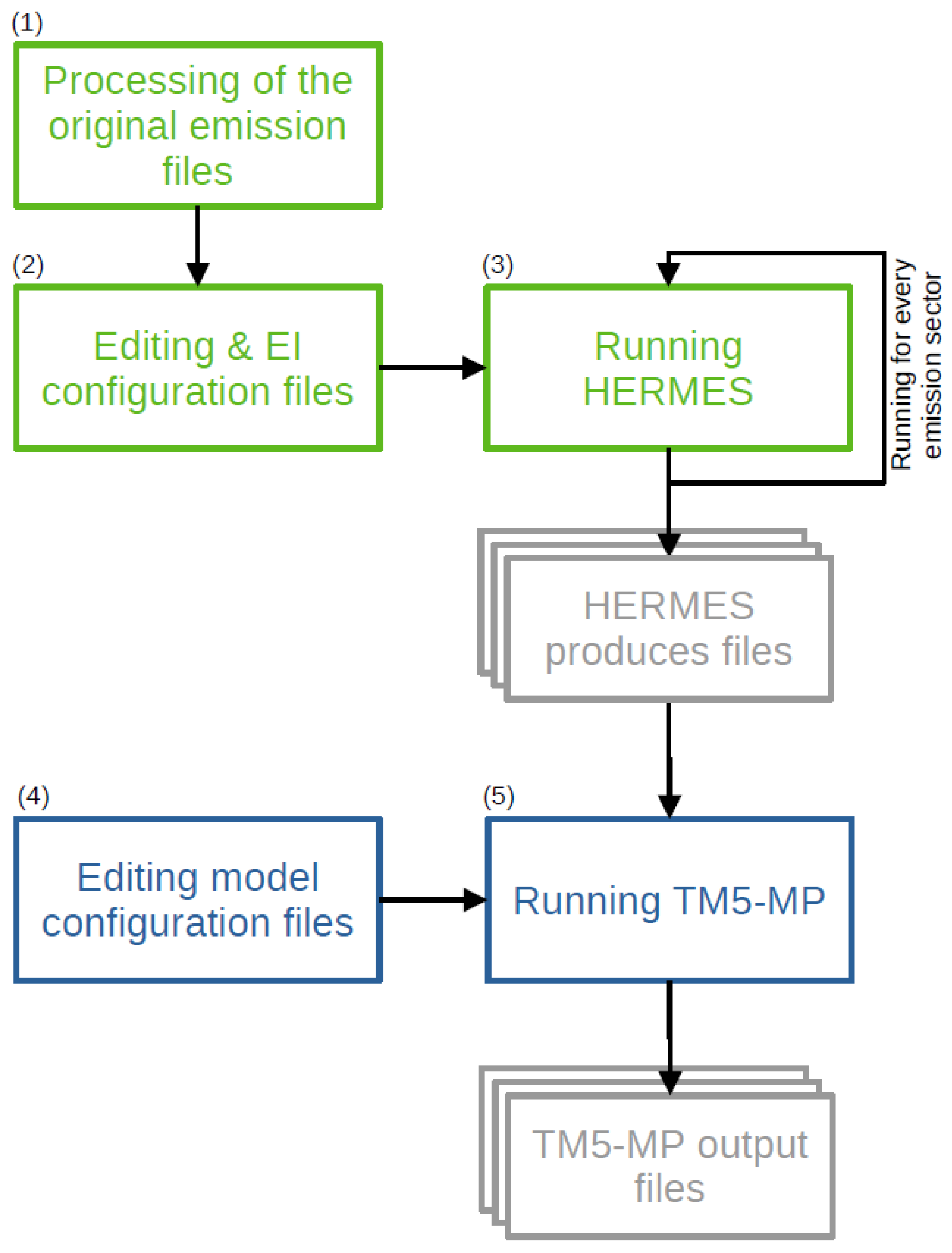
With these developments, HERMES and TM5-MP can now be used together. For the user this results in the workflow shown in Figure 1. Steps 1–3 were already explained in detail in Section 2.2 and summarized as follows:
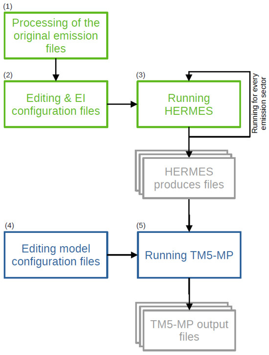
Figure 1.
Schematic representation of the workflow of HERMES (green) together with TM5-MP (blue) and the output files (gray). The numbers 1–5 indicate the five steps performed (compare Section 3.2).
- Processing original EI files;
- Preparing the EI configuration file and the HERMES configuration file;
- Running HERMES for each emission sector.
And expanded by the steps to be conducted in TM5-MP, namely the following:
- 4.
- Prepare model configuration files including newly added HERMES section;
- 5.
- Running TM5-MP.
3.3. Comparison to Old Workflow
3.3.1. Validation of Emission Amounts
To verify the quantities of pollutant emissions used in the newly developed TM5-MP-HERMES workflow, they were compared with the emissions used in the old workflow. For this comparison, the so-called emission budgets were used, which provide the emissions used during the simulation period. Both workflows should ideally generate identical pollutant emissions, resulting in equivalent emission budgets. Such a comparison allows the identification of any disparities in how the TM5-MP-HERMES system quantifies emissions of pollutants. Here, we utilize the relative difference, as defined by Equation (1) to assess any disparities. Emissions quantified through the old workflow are labeled ‘original’, while those processed through the new workflow are labeled ‘HERMES’.
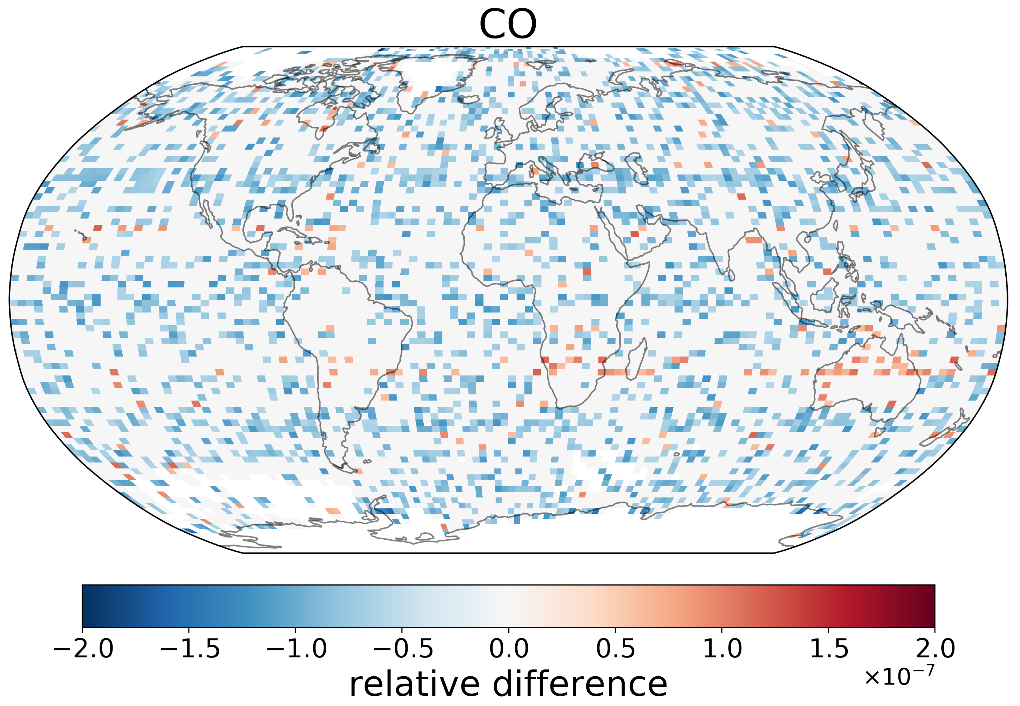
For the validation of emissions the first day of January 2016 was simulated. Anthropogenic emission data from CEDS, biomass burning data from GFED3, and natural emission data from MEGAN-MACC, LPJ_WHyMe and HYMN were used. Discrepancies were examined for all available species and are shown as examples for carbon monoxide (CO) in Figure 2. Figure 2 illustrates the relative differences between near-ground CO emissions in the two modeling results.
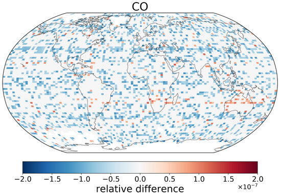
Figure 2.
Relative differences between carbon monoxide (CO) emissions quantified through the TM5-MP-HERMES system and the original workflow (without HERMES).
The comparison indicates an overall negligible difference typically on the order of 10−7, without significant spatial patterns. The noise-like variations in relative difference likely stem from the intermediate file-saving process at a resolution of 1° × 1° (longitude × latitude), the finest resolution at which TM5-MP can run. The regridding to a resolution of 3° × 2° or 6° × 4° is performed later in TM5-MP itself. In the original workflow, both regridding steps are performed during runtime, without intermediate saving. This intermediate saving step may contribute to the observed noise-like differences.
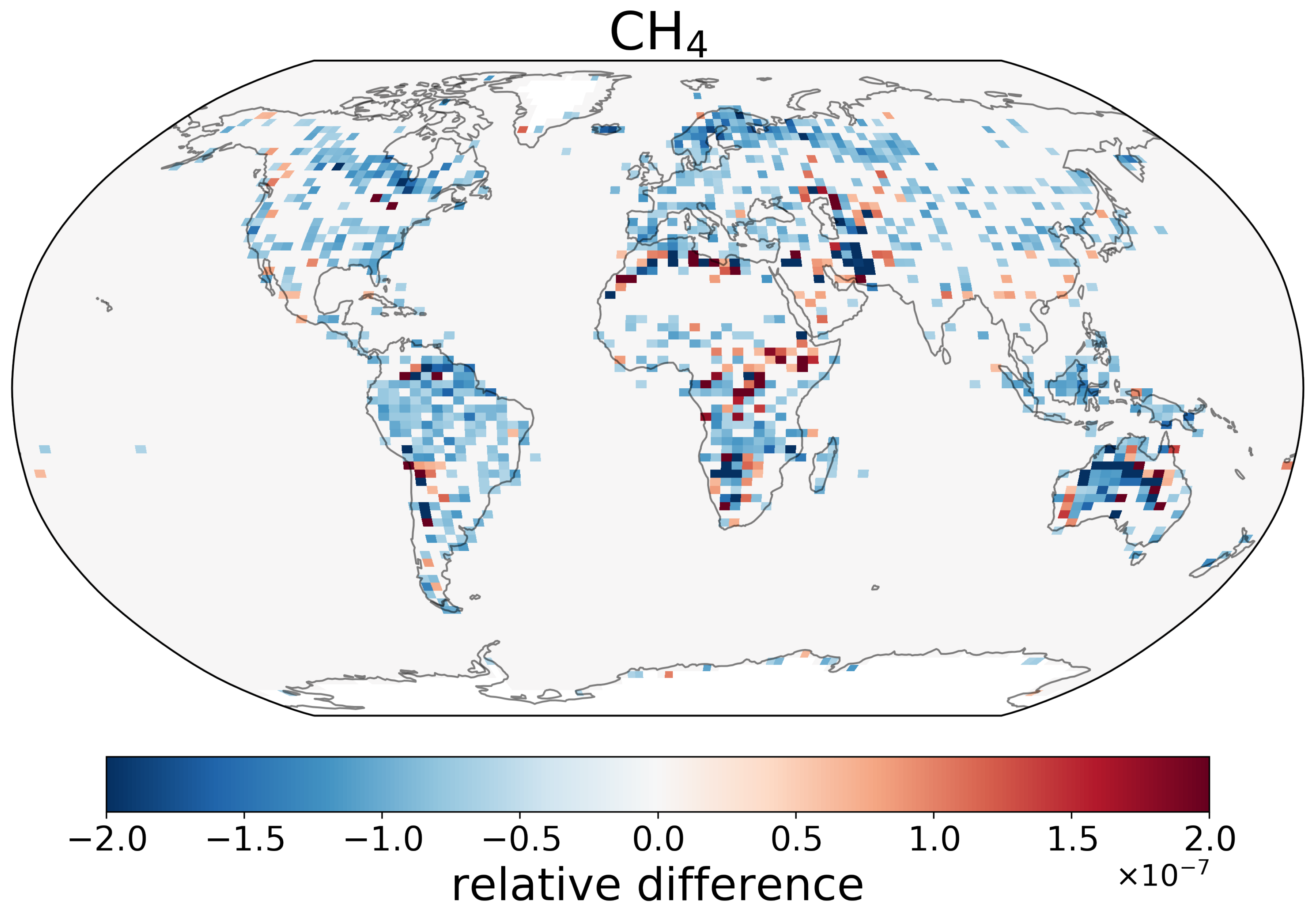
The patterns of relative differences for emissions of most other species are similar to those of CO, appearing as noise-like variations (see Figures S4–S7 for ethane, propane, and nitrogen oxide). The only exception is methane (CH4), as illustrated in Figure 3. For CH4, these patterns occur exclusively over land. The absence of these patterns over oceans can be attributed to the usage of HYMN data for ocean emissions. The HYMN dataset, which is available in 1° × 1° resolution, does not undergo resolution changes in HERMES, thus avoiding differences due to intermediate file-saving or slight discrepancies in regridding.
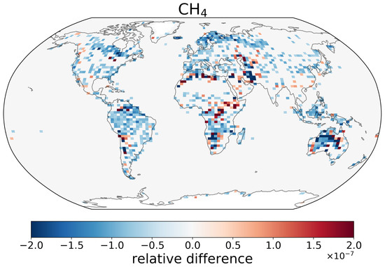
Figure 3.
Differences between the resulting CH4 budgets using the ‘original’ workflow (without the use of HERMES) and ‘HERMES’ workflow (with emission prepared through HERMES) relative to the results of the ‘original’ workflow.
3.3.2. Comparison of Computational Costs
To assess the computational costs of the newly implemented modifications, we analyzed the run times of two simulations: one with HERMES-produced data and one without. Both simulations utilized the setups described in Section 3.3.1, with the only difference being the extension of the simulation period to the full year of 2016. The simulations were conducted on the same system with identical settings.
In total, the run using HERMES took around 28 CPU minutes longer (corresponding to 0.5% of the total CPU run time) than the run without HERMES. Using 225 CPUs, which is the recommended amount of CPUs used for this resolution (3° × 2°) on this system (Aether HPC, details shown in S2 in the Supplementary Material), this leads to an increase of roughly 8 s per CPU and per month. However, it should be noted that additional time is needed for preprocessing the emission files through HERMES. This preprocessing adds approximately 30 min to the runtime for 1 year of data. This runtime of this process is highly dependent on factors such as the number of species and inventories prepared for the simulation, and the original horizontal resolution of the emission inventory. For example, preparing one year of LPJ data, which involves only one species (CH4), takes less than two minutes, whereas preparing 3D aircraft emission data from CEDS takes up to three hours per year.
Since the emission file preparation is separate from the main model run, running HERMES is necessary only once per case study. The emission files produced can then be reused in multiple simulations, offering an efficient and reusable workflow.
4. Case Study: EI Integration Using TM5-MP-HERMES and Model Setups
As mentioned earlier, emission preprocessors like HERMES offer a user-friendly and flexible platform for generating required EI files without extensive coding efforts. Therefore, it also enables easy integration of regional EIs into global ones, potentially leading to improved modeling performance over pollutant levels, as discussed in Section 1. In this study, we utilized the TM5-MP-HERMES system to integrate the REAS inventory into CEDS. We then compared the performance driven by this integrated anthropogenic EI with that of the initial CEDS inventory. This section provides the details of this case study, including the initial emission datasets and sectoral mapping between them, the creation of speciation profiles of non-methane volatile organic compounds (NMVOCs) emissions, and the setup of TM5-MP simulations and measurement data used for validation.
4.1. Initial Emission Datasets
In this case study, we utilized both the global EI CEDS and the regional EI REAS. CEDS provides historical emissions for the years 1750–2014, while REAS covers the years 1950–2015. Therefore, emission data from January 2012 until December 2014 were employed for both datasets. While all necessary steps for utilizing CEDS with HERMES have been completed beforehand (see Steps 1 and 2 in Section 2.2), these steps still need to be performed for REAS.
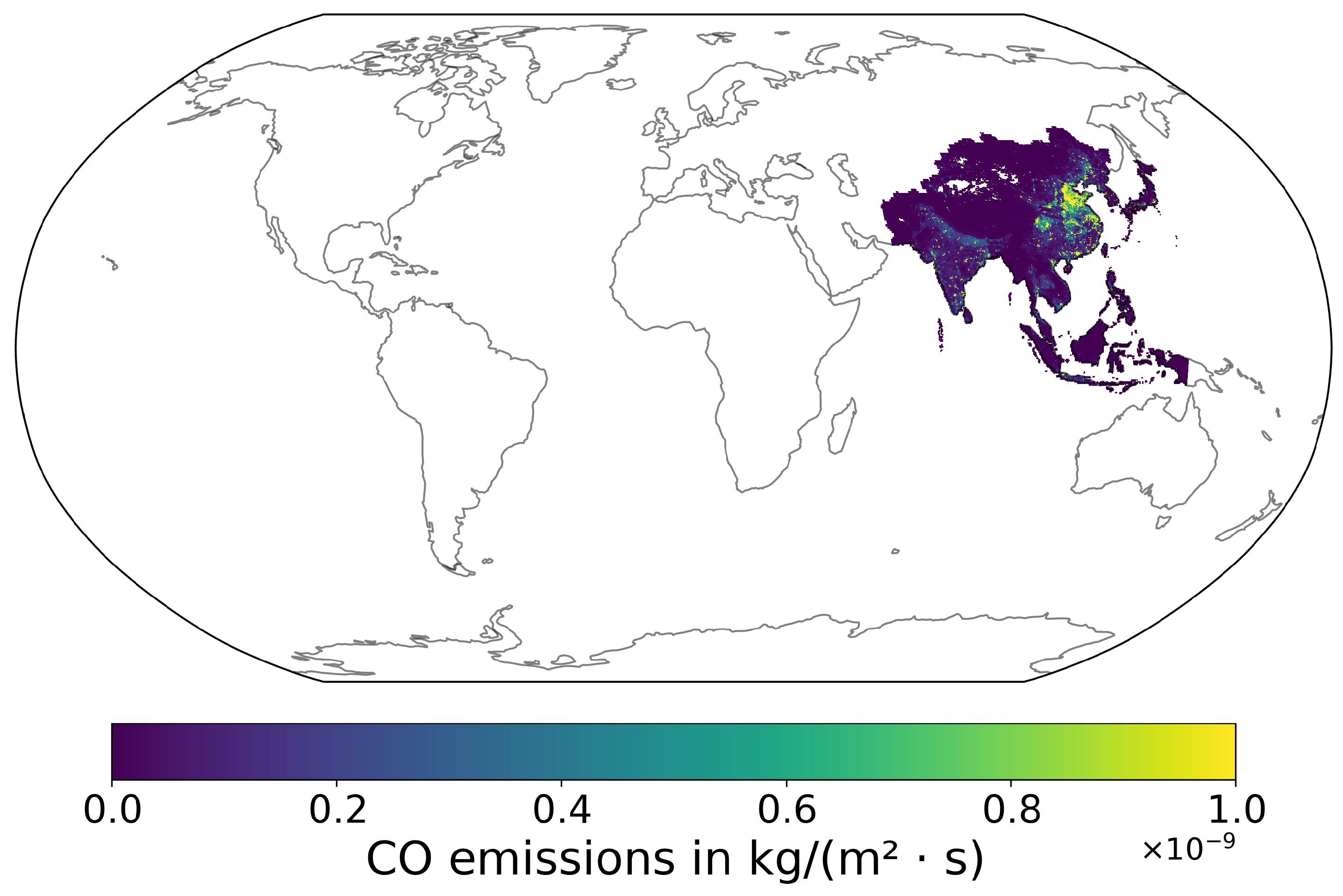
For this study, REASv3.2.1 data in gridded form were used. As a regional EI, it only contains emissions from countries within South, East- and Southeast Asia. To enable its use with HERMES, the EI is first introduced into an empty global grid. An example is shown for CO emissions from the industry sector in January 2012 in Figure 4. This step is part of Step 1, described in Section 2.2.

Figure 4.
Carbon monoxide (CO) emissions () from REAS in the industry sector for January 2012.
The unit transformation, mentioned in Step 1, is also applied to the REAS EI. To convert the provided data from units of to , knowledge of the grid cell area is required. However, the grid cell area of the REAS EI is not provided with the data. To address this, and considering that the REAS data are on a regular latitude–longitude grid with 0.5° × 0.5°, the grid cell area from the similarly gridded CMIP6 biomass burning data was used.
During the processing from HERMES into EIs usable in TM5-MP, another unit transformation into is performed (Step 2 in Section 2.2). Since the same grid cell areas are used in both transformations, the grid cell area cancels out.
With this methodology, the prepared emission data from REAS can now be used in HERMES for TM5-MP.
4.2. Sectoral Mapping between Two Inventories
The proper integration of REAS into CEDS using HERMES is controlled through its EI_configuation file, which specifies the emission sectors and species from both datasets that should be processed. To avoid double-counting of emissions in locations where data from both datasets are available, the ‘regrid mask’ option is employed. By using alpha-3 country codes, the emissions of a country can be enabled or disabled per inventory–sector combination. This way, during the construction of the EI_configuration file a double counting of emission can be prevented.
REAS and CEDS have different types of emission sectors. In order to integrate these two EIs, sectoral mapping is needed based on a standard definition of emission sector used in CMIP6 (same as that in CEDS). For each REAS sector the corresponding CMIP6 (sub-)sector was identified. When needed, multiple sub-sectors were added into the corresponding parent-sector, which is also used in TM5-MP. In cases were the CMIP6 parent-sector was not able to be reconstructed from REAS data alone due to missing sub-sectors or missing emissions in general. The CEDS emission sector was used instead. An example of this is the energy sector, where it could not be ensured that the REAS sector ‘Power Plant’ is equivalent to the CMIP6 energy sector. Since the provided sectors for REAS are dependent on the species, the sector mapping is dependent on this, too. The complete used sector mapping is shown in Table 1.

Table 1.
CMIP6 and REAS sector mapping.
4.3. Speciation Profile
The speciation profile set in the EI-configuration file serves as an indicator for HERMES, dictating which profile to use for transferring the provided species from the initial EI into pollutants used in the CTM. This process depends on the chemical mechanism employed. For datasets like CEDS and other datasets used previously, the speciation was translated from internal source files of TM5-MP into speciation profiles compatible with HERMES. The speciation profile is also used to select which pollutants should be provided from which inventory–sector combination, enabling the use of different inventories per sector and region depending on the pollutant. This way, the agriculture sector can use REAS data for ammonia in the REAS-regions, while using CEDS data for all other pollutants.
For REAS, only the speciation of NMVOCs is needed for the use with the mCB05 chemical mechanism of the TM5-MP model. However, REAS pollutants were not provided in the commonly used 25 different VOCs defined by the Global Emission InitiAtive (GEIA), for which a mapping into CB05 species already exists in the TM5-MP model, aligning with the speciation used for CEDS data. Additionally, conversion factors or molecular weights for the REAS species were not provided.
Therefore, a third dataset, the emission mosaic of the ‘Task Force on Hemispheric Transport of Air Pollution’, the HTAPv3 [28], was used to create a speciation profile. HTAPv3 is an emission mosaic that also utilizes the REAS dataset for the corresponding region of East, South and Southeast Asia. HTAPv3 provides a speciation profile for the aforementioned 25 GEIA VOCs. With the assistance of this speciation profile, the NMVOC pollutants provided in REAS were converted into 25 GEIA VOCs for the relevant sectors. For final mapping into pollutants needed in TM5-MP, the same conversion as for the CEDS dataset is used.
4.4. Experimental Setup
To investigate the effect of integrating a regional EI into a global one, the newly developed TM5-MP-HERMES system was used. Anthropogenic emissions from REAS were integrated into CEDS with the help of HERMES (referred to as ‘with REAS’ from now on), and CEDS alone (referred to as ‘without REAS’ from now on) was also prepared through HERMES, and then used in the TM5-MP CTM. For biomass-burning and natural emissions, the ‘old’ workflow was used using the same emissions, as described in Section 3.3, expanded by data from MACC. For the simulations of TM5-MP, the CTM was driven by ERA-Interim meteorology and using the mCB05 chemical mechanism on a horizontal resolution of 3° × 2° degrees (longitude × latitude) and 25 hybrid vertical levels. The relatively coarse resolution is a compromise between computational time needed for the simulation and the horizontal resolution necessary to be able to observe the effect of the usage of different emission inventories. Both simulations were used to produce monthly mean output concentrations from January 2012 to December 2014, with the first year used as spin-up.
The updated TM5-MP, along with the modified HERMES codes used in this work, can be accessed online [29]. Additionally, the emission files produced by HERMES for this study, aggregated over all sectors, are also available online for specified species (CO, NOx, C2H6, and C3H8) [30]. Per-sector files for all species can be provided upon request.
4.5. Measurement Data Used in Validations
In order to validate the model results, ground-based measurements of pollutant mixing ratios at multiple sites all over the world were used. Specifically, measurements for carbon monoxide (CO), ozone (O3), ethane (C2H6), propane (C3H8), and nitrogen dioxide (NO2) were used. The sources of the measurement data are mostly regional and national air quality monitoring networks, of which the details can be found in Section S3.1 of the Supplementary Materials. The locations of the measurement sites for each species are displayed in Supplementary Figures S7–S10.
For comparison with the model, monthly mean data are needed. For this purpose, it is required to calculate their monthly average of the measurements data that were provided in either hourly or daily temporal resolution. The hourly initial data were averaged first to daily, then to monthly. From the daily initial data, the corresponding monthly data was directly calculated. If over one-third of the hourly data in a day or over one-third of the daily data in a month are missing, these data would be discarded from the comparisons.
5. Case Study: Results and Discussion
To evaluate the model performance driven by the integrated EIs and the initial CEDS, we compared the simulated mixing ratios of CO, C2H6, C3H8, NO2 and O3, in both simulations with and without REAS to near-ground measurements. These species were selected to assess the changes in concentrations resulting either directly from the replacement of CEDS by REAS in part of Asia (CO and NO2), or indirectly (O3). Additionally, we examined whether the use of REAS data could improve the agreement of the simulated concentrations of two VOCs (C2H6 and C3H8) that were underestimated in the past [7].
5.1. Carbon Monoxide
CO is a primary pollutant with emissions as its main sources in the atmosphere. For its emissions in South, East and Southeast Asia, REAS exhibits, averaged over the years 2012–2014, were around 0.03% higher CO emissions than CEDS for the same region. Figure S11(left) in the Supplementary Materials shows that the relative differences in CO emissions between CEDS and REAS are not evenly distributed. Specifically, CEDS gives higher emissions for western China, whereas REAS gives significantly higher emissions for Mongolia. REAS also shows mainly higher emissions in eastern China. Furthermore, single grid cells scattered all over Southeast Asia show significantly higher emissions in REAS. Integrating REAS into CEDS changes both the amount and spatial distribution of CO emissions in Asia. Thereby, the simulations by TM5-MP are likely to produce different CO fields not only within Asia, but also globally. The resulting concentrations from the two simulations were validated, and it was assessed whether the usage of REAS leads to an improvement in model performance. The simulated CO mixing ratios were compared to the measurements from (a) remote areas with flasks measurements from the National Oceanic and Atmospheric Administration (NOAA) and (b) measurements from various data sources mostly located at urban/suburban places. A map of the stations’ location, divided into remote stations and urban stations inside Asia (specifically, the REAS area) and outside of Asia, is shown in Figure S7 in the Supplementary Materials with an overview of the utilized data sources. The processing is described in Section 4.5.
5.1.1. Model Performance at Remote Stations
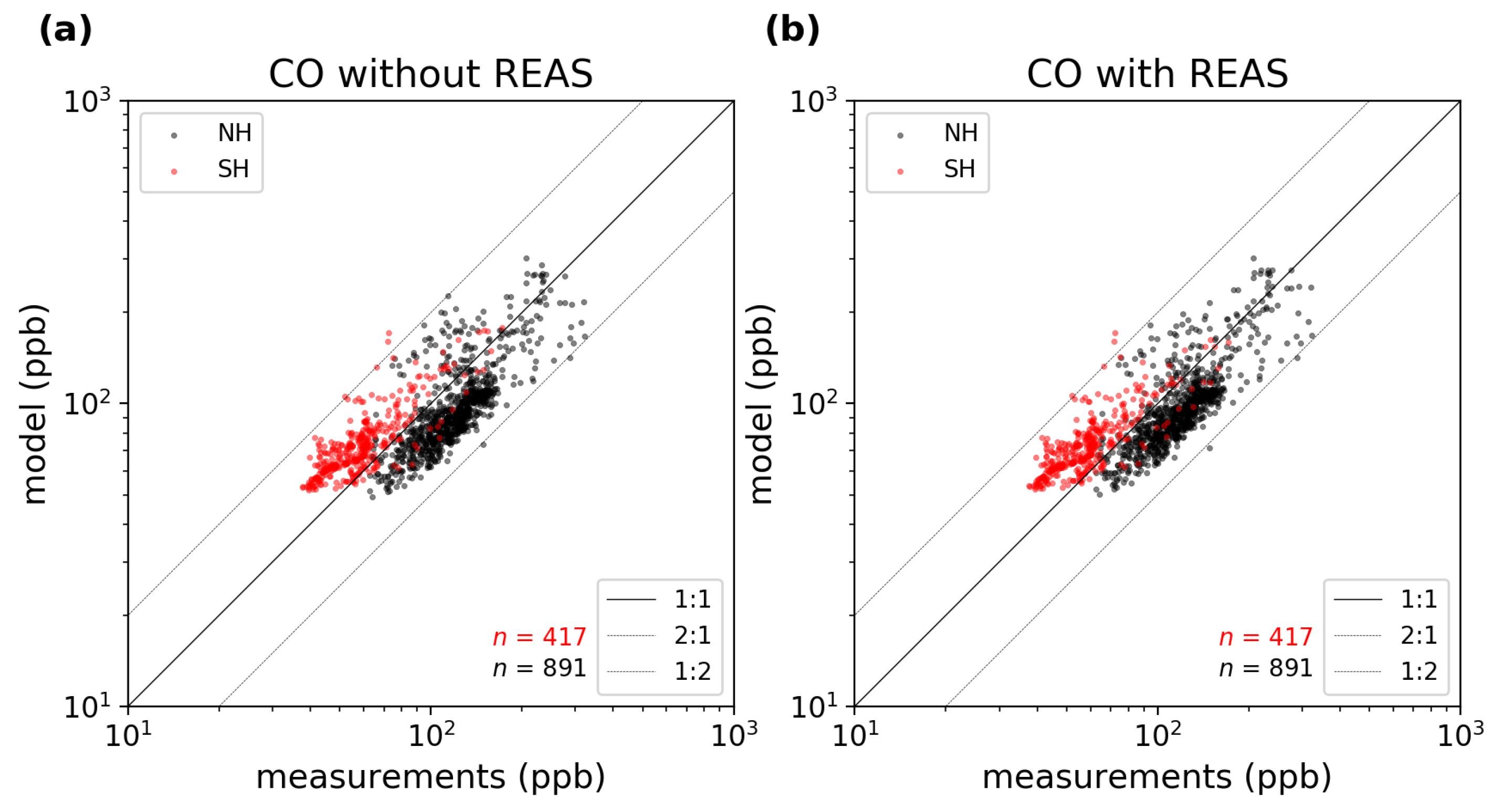
Figure 5 shows the comparison between the model results and the corresponding measurements at remote stations. Since remote areas are less influenced by human activities, comparisons with measurements at remote stations aim to indicate the performance of our model in simulating the background levels of CO. The stations are split into those in the Southern Hemisphere (SH, in red) and the Northern Hemisphere (NH, in black). Overall, CO mixing ratios are underestimated in the NH and overestimated in the SH. The inclusion of REAS data results in a slight increase in the modeled global mixing ratio of CO in the NH. To quantify and compare model performance with and without REAS, four statistical metrics were used, which include mean bias (MB), normalized mean bias (NMB), the slope, and correlation factors between model results and observations. The formulas to quantify these metrics can be found in Section S5.1 in the Supplementary Materials.
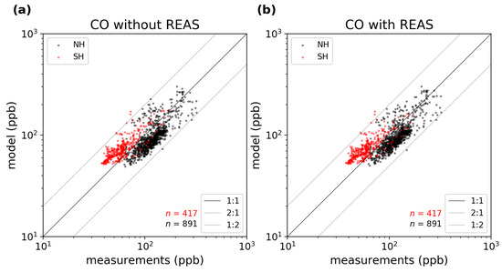
Figure 5.
Comparison between monthly mean near-surface CO observations with corresponding model results. The comparisons are separately made for stations in the Northern (NH, in black) and Southern Hemisphere (SH, in red). The results in the simulation without and with REAS are shown in the panel (a) and (b), respectively. In both plots, the solid black line is the 1:1 line, while the dashed lines are the 1:2 and 2:1 lines.
The statistics in Table 2 suggest slight reductions in the MB and NMB values in the NH, along with increasing correlations between observational and modeled CO. In detail, the MB decreases from −22 ppb(−18%) to −20 ppb(−17%). The slope is improving from 0.76 to 0.78 with the integration of REAS into CEDS and the correlation improves from 0.74 to 0.78. Thus, integrating REAS into CEDS results in a slight improvement in the model performance for CO in the NH, particularly in remote regions. However, the mean bias and normalized mean bias indicate that the agreement between model and measurements remains unchanged with the implementation of REAS for the SH. Since most changes for REAS are applied in the NH. This result meets the expectations.
Table 2.
Statistics for the model performance of CO in comparison to measurements at remote stations.
5.1.2. Model Performance at Urban Stations
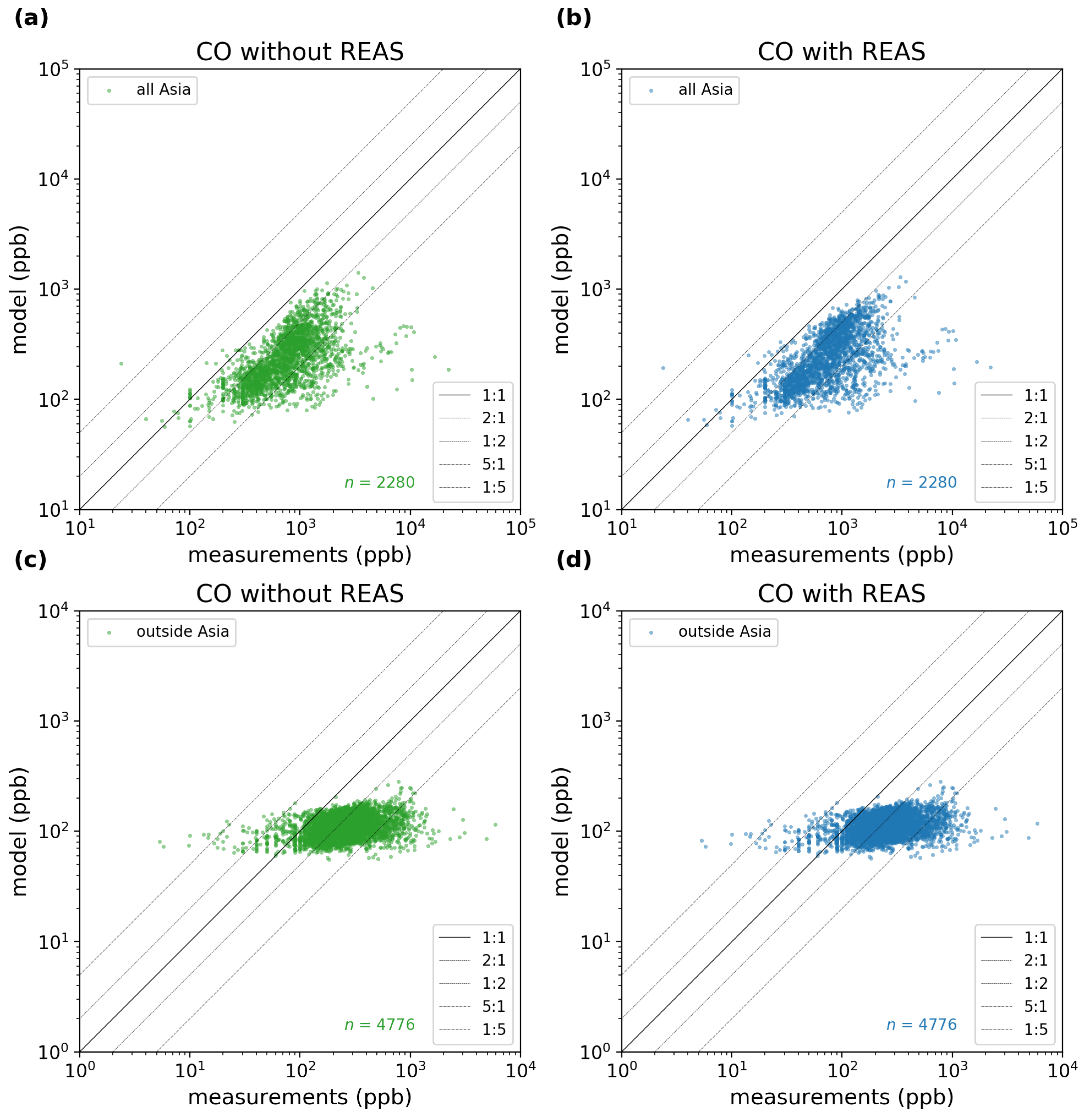
In addition to the evaluation of model performance at remote stations, we also conducted comparisons between simulated CO mixing ratios with measurements in urban areas. Since urban CO is mainly due to high local emissions, model performance at urban stations could directly indicate the accuracy of CO emissions in EIs. To investigate the influence of EI integration, we separately evaluated the model performance of CO in and outside of Asia. The results are presented in Figure 6 while the statistics are listed in Table 3.
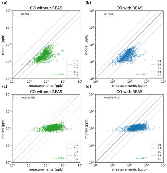
Figure 6.
Comparison between modeled and measured surface CO mixing ratio. The four panels present the comparisons inside (a,b) and outside (c,d) Asia for model runs with (b,d) and without (a,c) REAS. In all plots, the solid black line is the 1:1 line, while the dashed lines are the 1:5, 1:2, 2:1, and 5:1 lines.
Table 3.
Statistics for the model performance of CO in comparison to measurements at mostly urban stations.
Results show that the TM5-MP model underestimates CO mixing ratios in urban regions both within and outside of Asia by over 50%. It should be noted that the spatial resolution selected for these simulations is only 3° × 2°, which is too coarse to properly describe the urban scale emission activities, transport, and other atmospheric processes. Hence, in order to improve model performance of CO at urban stations, spatially finer simulations are needed. Regardless of this limitation, the difference in model performance for urban CO in the two cases suggests improvement by using the integrated EIs, especially in the highly populated areas of Asia. The reduced underestimation of CO in urban regions is also represented by the improved MB and NMB. With REAS, the bias (NMB) changes from −684 ppb (−72%) to −678 ppb (−71%) at urban sites within Asia, and from −184 ppb (−62%) to −183 ppb (−62%) outside of Asia.
Overall, it is evident that the agreement between the model and measurements of CO is poor at urban stations both inside and outside Asia. The correlation between model results and measurements of CO at urban stations is noticeably worse compared to the one at remote stations. While the MB improves slightly with the use of REAS data, the correlation slightly worsens (r2 = 0.30 compared to r2 = 0.28 in Asia and r2 = 0.23 compared to r2 = 0.22 outside Asia). The slope is in all cases already very close to zero (0.03–0.05) so that any changes, if present, are not significant.
The model produced CO mixing ratio, both at remote and urban stations, is slightly affected by the integration of REAS data. The bias in all cases outside of the SH is improving; however, these improvements are still within the uncertainties. Nonetheless, it appears that the inclusion of a regional dataset as REAS can improve the model performance for CO.
5.2. Ethane and Propane
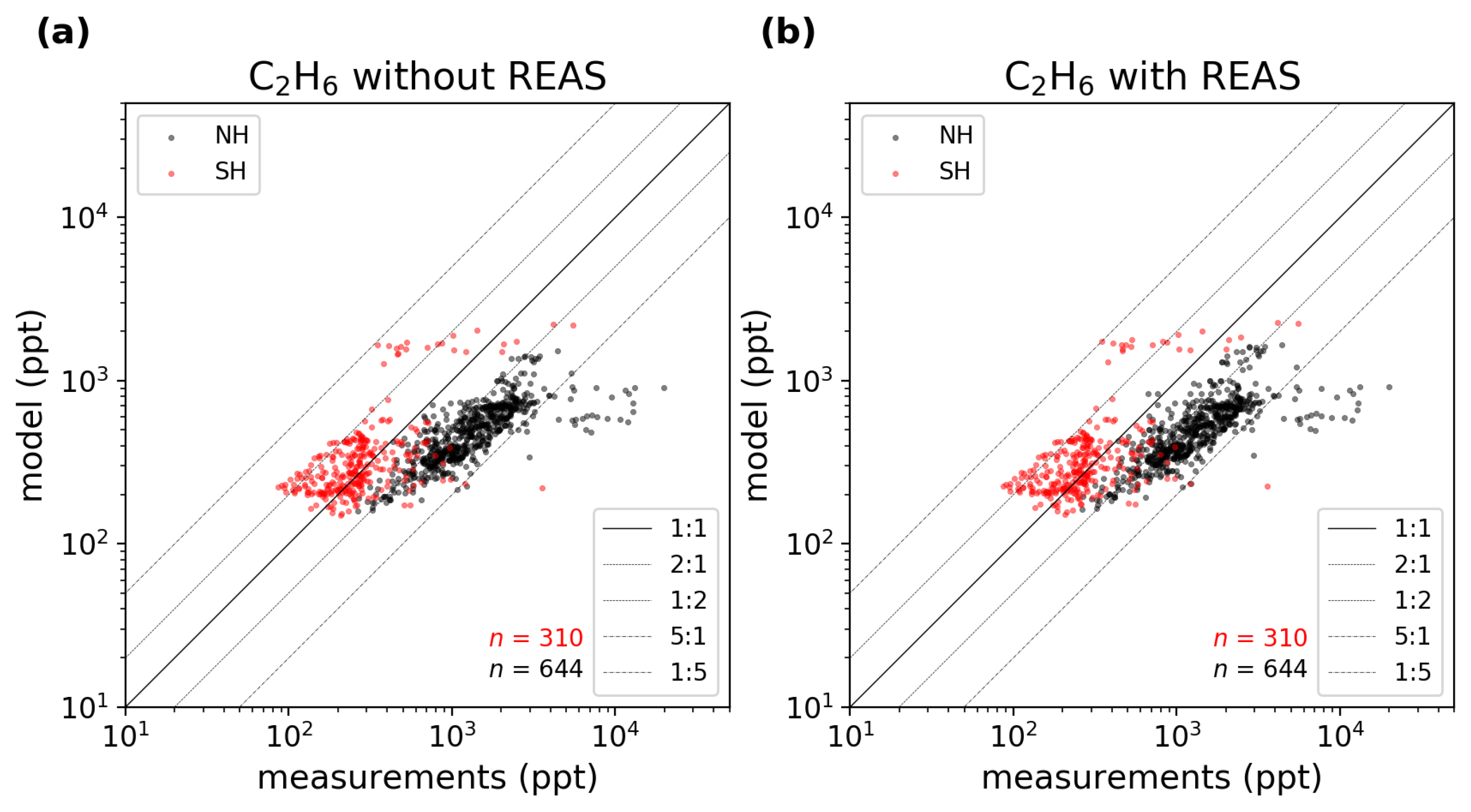
The same analysis as for CO was performed for ethane (C2H6) and propane (C3H8). The levels of these two VOCs were largely underestimated in previous modeling studies using TM5-MP [7]. Since both VOCs are introduced in the atmosphere primarily due to direct emissions, we investigated if an increase in VOC emissions in East Asia improves the agreement between observed and modeled C2H6 and C3H8. We used flask measurements of C2H6 and C3H8 by NOAA for the comparisons. The locations of the used stations are shown in Figure S8 in the Supplementary Materials.
Figure 7 shows the comparison between measured and simulated monthly-mean surface concentrations of C2H6 at remote stations. When driven by the initial CEDS EI, a clear underestimation of C2H6 levels can be found in the NH, while the simulated results in the SH are overall acceptable (Figure 7a). The integration of REAS into CEDS leads to slightly higher C2H6 concentrations in the NH in the simulations, indicating an improvement in the model’s overall performance for simulating C2H6 (Figure 7b). Statistics listed in Table 4 indicate that after integration of REAS, the mean bias of C2H6 mixing ratios in the NH decreases from −1151 ppt to −1140 ppt, or from −69% to −68% expressed as a percentage. In the SH, higher C2H6 emissions by the integration of REAS leads to increasing mixing ratios of C2H6 and thereby higher overestimation of C2H6 (30 ppb (8%) compared to 37 ppb (10%)). The correlation decreases for the NH (0.48 to 0.44) and does not change at all for the SH (0.60) with the inclusion of REAS data into CEDS. The slope in the NH is the same in both cases (0.06), with and without REAS, while a marginal improvement for the SH is visible (0.45 to 0.46).
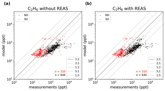
Figure 7.
Comparison between the measured and modeled monthly-mean near-surface concentrations of ethane (C2H6). The results were split in stations in the Northern Hemisphere (NH, in black), and the Southern Hemisphere (SH, in red). The results in the simulation without and with REAS are shown in the panel (a) and (b), respectively. The solid black line is the 1:1 line, while the dashed lines are the 1:5, 1:2, 2:1, and 5:1 lines.
Table 4.
Statistics for C2H6 with and without REAS for the SH and NH.
The slope estimated for the NH is highly impacted by model results of C2H6 in the Southern Great Plains, USA. The modeled mixing ratios at this station are strongly underestimated compared to observations by almost one order of magnitude. High values of C2H6 mixing ratios indicate strong nearby emissions, not being resolved in either the coarse modeling resolution of 3° × 2° or already the anthropogenic EI files. A further analysis with higher horizontal resolution combined with more spatially spread measurements in that region would give more insight.
For C3H8, a similar improvement of model performance by integrating REAS as C2H6 can also be found (Figure S13 and Table S1). The bias of C3H8 mixing ratios reduces from −1543 ± 1672 ppt to −1464 ± 1676 ppt in the NH. In the SH, the slope improves from 0.14 to 0.25 with the use of REAS.
Overall, these results show that the inclusion of REAS yields, as observed for CO, only small changes of the model performance of C2H6 and C3H8 at remote stations. As for CO the main reason for this is the large distance of the introduced changes in Asia to the positions of the remote stations.
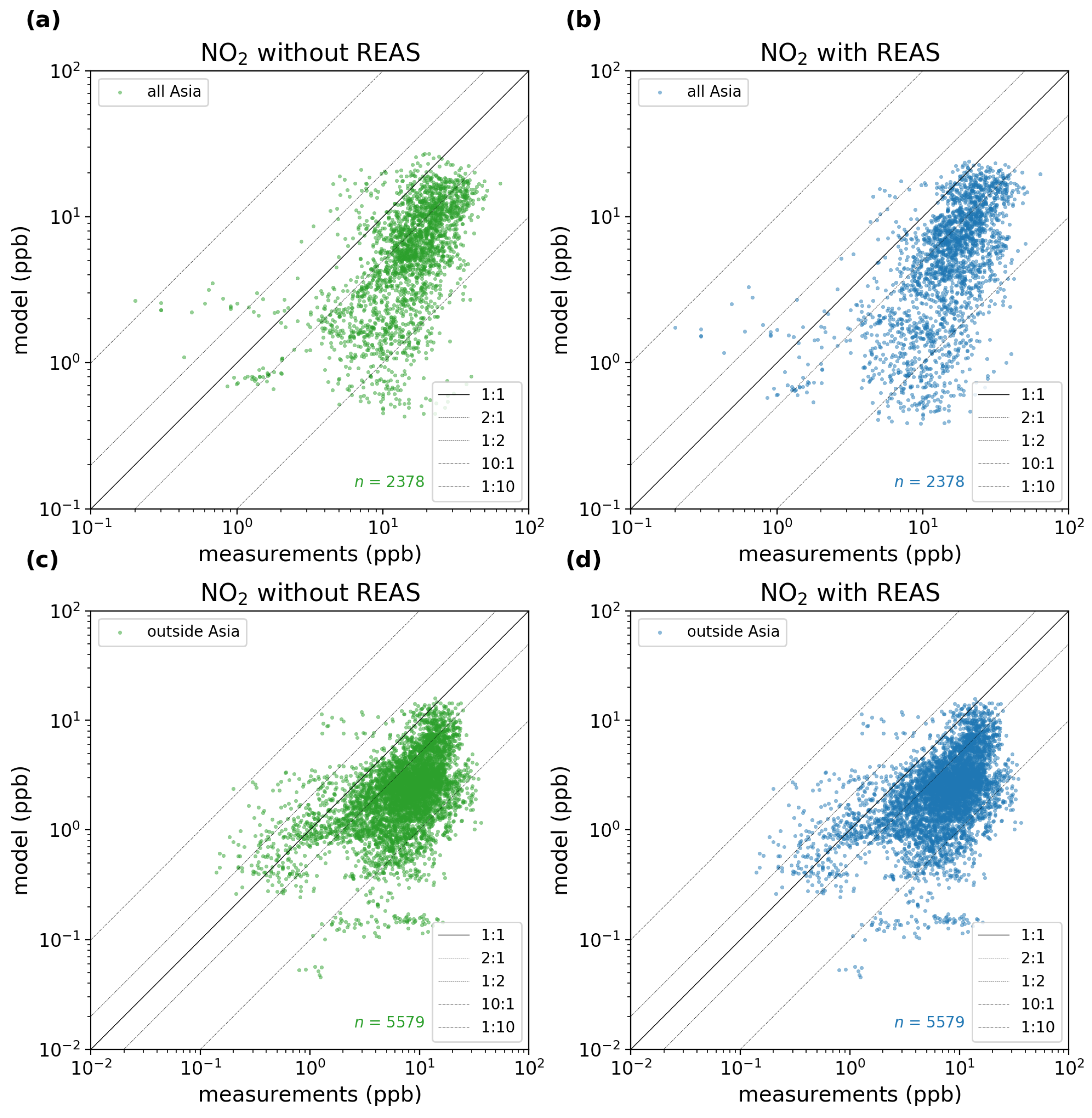
5.3. Nitrogen Dioxide
Another important pollutant in terms of air quality is nitrogen dioxide (NO2). Similar to previous evaluations of model performance, modeled NO2 was also compared to measurements at various urban stations worldwide. The location of these stations and the dataset sources are presented in the Supplementary Materials, Section S3. NO2 atmospheric levels are closely linked to nearby emissions due to the short lifetime of 2 to 8 h for NOx [31]. Therefore, to examine the influence of EI integration on NO2 simulations, model performance at sites within and outside of Asia is separately discussed in this section.
Figure 8 shows the comparison between measured and modeled surface mixing ratios of NO2. We found that overall, our model underestimates NO2. At some sites, the simulated levels of NO2 are underestimated by up to one order of magnitude. This underestimation can be explained mainly by the coarse model resolution in combination with often very localized NOx sources. This also leads to comparable small impacts of the integrated EI on global, monthly NO2 mixing ratios.
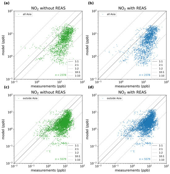
Figure 8.
Comparison between modeled at measured surface NO2 mixing ratio. Shown are comparisons inside (a,b) and outside (c,d) Asia for model runs with (b,d) and without (a,c) REAS. In all plots, the solid black line is the 1:1 line, while the dashed lines are the 1:5, 1:2, 2:1 and 5:1 lines.
For stations within Asia, the analysis reveals that locations having a higher mixing ratio of NO2 are better represented by the model compared to those with lower mixing ratios. With the use of REAS data, the scatter plot reveals a division into two distinct clusters, indicating that some stations are affected more by changes in emissions than others. Contrary to what was observed for CO, the existing underestimation is slightly amplified for NO2. This stems from the fact that the NOx emissions provided from REAS are, averaged over the REAS region from 2012 to 2014, lower by −0.43% than those provided by CEDS. This can be seen in the relative differences between REAS and CEDS, discussed in Section S4 of the Supplementary Materials.
The reduction in NOx input emissions may contribute to a further decrease in modeled NO2 when using REAS instead of CEDS. Additionally, the split observed in the scatter plot upon the introduction of REAS data can be attributed to the relative difference in emissions between REAS and CEDS. Specifically, while emissions in China appear to be mostly higher in REAS, in India NO2 emissions from REAS are smaller.
Overall, using REAS data enhances the model’s underestimation at stations in Asia by 2%, while the model performance remains consistent with and without REAS for stations outside Asia, which is expected due to the short lifetime of NOx. Moreover, the slope and correlation metrics do only show minimal improvement with the use of REAS. The summarized statistics can be found in the Supplementary Materials, Table S2.
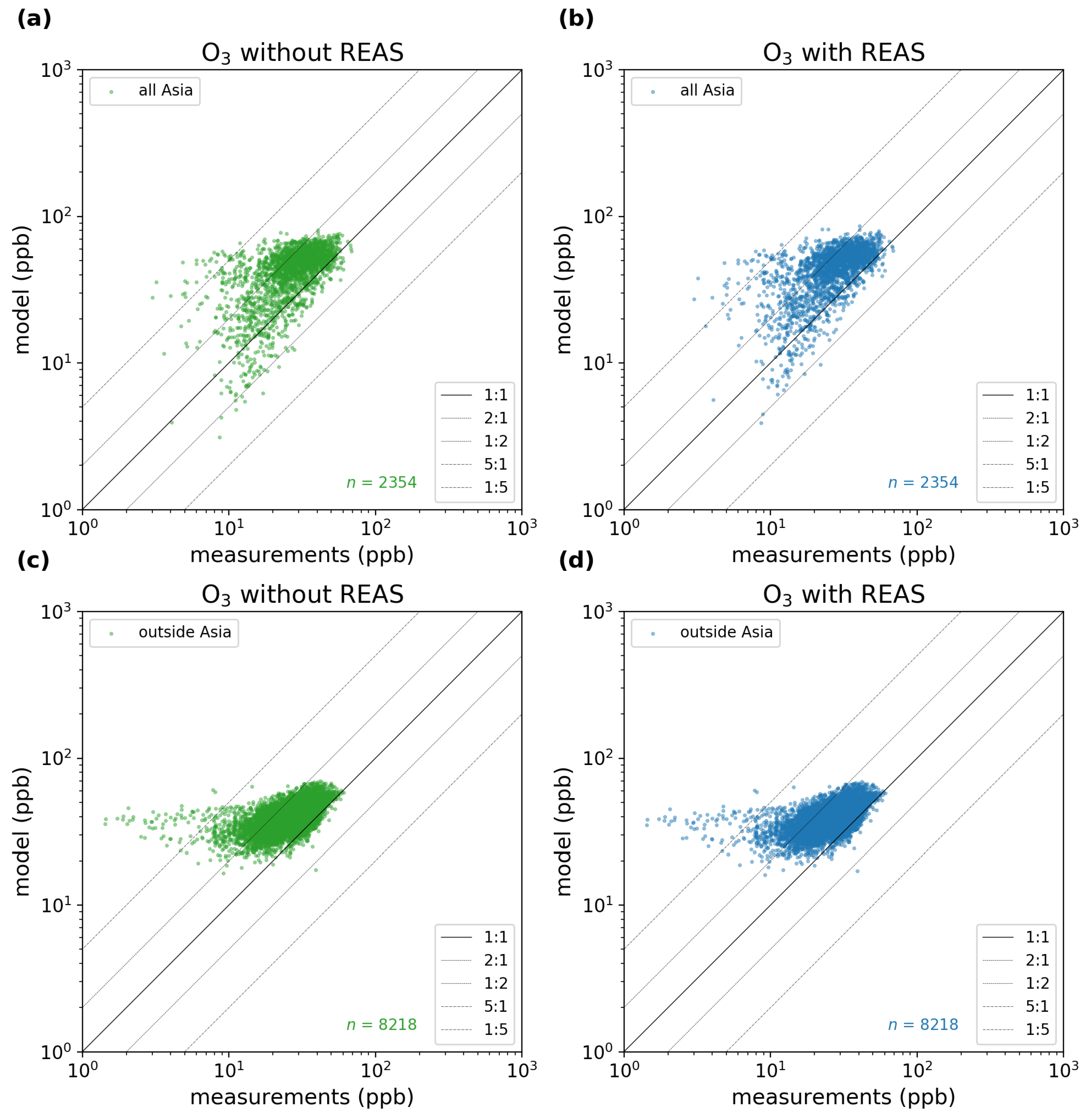
5.4. Ozone
The last species evaluated against measurements in this study is ozone (O3). In contrast to the other species examined earlier, which are primary pollutants directly emitted into the atmosphere, ozone is a secondary pollutant, produced from its precursors (mainly NOx, VOCs and CO) through complex non-linear photochemistry in the troposphere. Therefore, changes in emissions due to the integration of REAS can also lead to changes in the simulated ozone quantities.
Figure 9 illustrates the comparison between modeled and measured surface-level ozone mixing ratios at urban stations. The locations of the stations are shown in Figure S10 in the Supplementary Materials. Stations were categorized into those inside Asia and, therefore, close to the introduced changes, and those outside Asia. The use of REAS leads to increased overestimation of O3 in the model, that can be attributed to the amplified underestimation of NO2. Past observations have shown that China’s Clean Air Action Plan, aimed at effectively mitigating NOx emissions, led to an increase in ozone pollution when VOCs emissions were not concurrently reduced [32,33]. This was also observed during COVID-19 lockdowns in China [34]. This increase in ozone is also noticeable for stations outside Asia, although to a lesser extent.

Figure 9.
Comparison between modeled and measured surface O3 mixing ratio. The four panels present the comparisons inside (a,b) and outside (c,d) Asia for model runs with (b,d) and without (a,c) REAS. In all plots, the solid black line is the 1:1 line, while the dashed lines are the 1:5, 1:2, 2:1, and 5:1 lines.
Inside Asia, the MB of the levels of ozone changed from 15 ppb (54%) to 17 ppb (59%) with the integration of REAS into CEDS. For stations outside Asia and, therefore, more distant to the introduced changes, a decrease from 14 ppb (50%) to 13 ppb (48%) is observed. Furthermore, the slope and correlation in all cases is only affected slightly. The detailed statistics can be found in Table S3 in the Supplementary Materials.
6. Conclusions and Outlook
In this paper, we introduced the coupling of the TM5-MP CTM to the emission preprocessor HERMES, offering enhanced capabilities for users to manipulate emission datasets. The integration of HERMES facilitates the seamless substitution of global emission data with regional datasets, opening avenues for diverse emission scenarios. We demonstrated this capability by combining the global dataset CEDS with the regional emission dataset for Asia, REAS.
To achieve this integration, we developed a preprocessor for HERMES compatible with the REAS dataset, established speciation profiles for each sector and dataset, and configured an integrated EI using spatial masks in a simple CSV file. The combined emission data were then used to run TM5-MP from 1 January 2012 until 31 December 2014, excluding the first year as spin-up. Subsequent comparisons with measurements aimed to discern changes in global air quality resulting from the updated input emissions.
For carbon monoxide, we observed an slight improvement in the modeled mixing ratios at remote stations with the use of REAS. However, for stations closer to densely populated areas, a marginal decrease in bias was observed, while the slope and Pearson correlation of the linear fit were slightly worsened. This can be attributed to the relatively coarse model resolution of 3° × 2°.
The underestimation of ethane was mitigated for remote stations in the Northern Hemisphere with the implementation of REAS data, while the Southern Hemisphere experienced an augmentation to the existing overestimation.
Nitrogen dioxide analysis revealed a contrary pattern, where the existing underestimation at urban stations in Asia decreased with REAS data due to lower NOx emissions compared to CEDS. The reduction in NO2 in the Asian region led to an increase in the overestimation of ozone, aligning with observations of ozone rise during NOx reductions in China, such as those observed during COVID19 lockdowns.
In summary, our findings highlight the slight positive impact of REAS data on model performance, particularly for remote stations. The resolution of 3° × 2°, however, proved insufficient to capture small, highly polluted areas in urban settings.
Supplementary Materials
The following supporting information can be downloaded at https://www.mdpi.com/article/10.3390/atmos15040469/s1, Figure S1: Flowchart for TM5-MP; Figure S2: Flowchart for HERMES; Figure S3: Flowchart for TM5-MP with new workflow; Figure S4: Differences between the resulting C2H6 budgets using the ‘original’ workflow (without the use of HERMES) and ‘HERMES’ workflow (with emission prepared through HERMES) relative to the results of the ‘original’ workflow; Figure S5: Differences between the resulting C3H8 budgets using the ‘original’ workflow (without the use of HERMES) and ‘HERMES’ workflow (with emission prepared through HERMES) relative to the results of the ‘original’ workflow; Figure S6: Differences between the resulting NOx budgets using the ‘original’ workflow (without the use of HERMES) and ‘HERMES’ workflow (with emission prepared through HERMES) relative to the results of the ‘original’ workflow; Figure S7: Location of CO measurement stations used for validation. Orange dots are representing NOAA stations (‘remote’), while blue dots are showing stations closer to polluted regions; Figure S8: Location of C2H6 and C3H8 NOAA measurement stations used for validation; Figure S9: Location of stations used for validation with NO2 measurement data; Figure S10: Location of stations used for validation with O3 measurements; Figure S11: Relative difference between REAS and CEDS for CO and NO2, averaged over the year 2012–2014; Figure S12: Relative difference between REAS and CEDS for C2H6 and C3H8, averaged over the year 2012–2014; Figure S13: Comparison between the measured and modeled monthly-mean near-surface concentrations of ethane (C3H8); Table S1: Sources of Measurements used; Table S2: Statistics for the model performance of C3H8 in comparison to measurements at remote stations; Table S3: Statistics for the model performance of NO2 in comparison to measurements at urban stations; Table S4: Statistics for the model performance of O3 in comparison to measurements at urban stations.
Author Contributions
Conceptualization, M.V., N.D. and S.-L.S.; methodology, N.D. and S.-L.S.; software, S.-L.S.; validation, S.-L.S. and K.Q.; formal analysis, S.-L.S.; investigation, S.-L.S.; resources, K.Q.; data curation, K.Q. and S.-L.S.; writing—original draft preparation, S.-L.S.; writing—review and editing, M.V. and N.D.; visualization, S.-L.S.; supervision, M.V. and N.D. All authors have read and agreed to the published version of the manuscript.
Funding
N.D. and S.-L.S. are funded by the DFG, German Research Foundation under Germany’s Excellence Strategy (University Allowance, EXC 2077), S.-L.S. was funded by the University of Bremen. K.Q. was funded by the University of Bremen. K.Q. was funded by the DFG-NSFC Sino-German AirChanges project (grant No. 448720203).
Institutional Review Board Statement
Not applicable.
Informed Consent Statement
Not applicable.
Data Availability Statement
The analysis was conducted using python. The Jupyter Notebooks are available at https://dx.doi.org/10.5281/zenodo.10731412, accessed on 8 April 2024. The model and emission data used here are available at https://dx.doi.org/10.5281/zenodo.10731633, accessed on 8 April 2024. The version of TM5-MP that uses HERMES produced emission files can be found at https://dx.doi.org/10.5281/zenodo.10731687, accessed on 8 April 2024. The updated HERMESv3_gr emission preprocessor for producing emission files for TM5-MP is available here: https://dx.doi.org/10.5281/zenodo.10732245, accessed on 8 April 2024.
Acknowledgments
The simulations and analyses were performed on the HPC cluster Aether at the University of Bremen, financed by DFG within the scope of the Excellence Initiative. MV acknowledges support by the DFG, German Research Foundation under Germany’s Excellence Strategy (University Allowance, EXC 2077).
Conflicts of Interest
The authors declare no conflicts of interest.
References
- Brasseur, G.P.; Jacob, D.J. Modeling of Atmospheric Chemistry; Cambridge University Press: Cambridge, UK, 2017. [Google Scholar] [CrossRef]
- Madrazo, J.; Clappier, A.; Belalcazar, L.C.; Cuesta, O.; Contreras, H.; Golay, F. Screening differences between a local inventory and the Emissions Database for Global Atmospheric Research (EDGAR). Sci. Total Environ. 2018, 631–632, 934–941. [Google Scholar] [CrossRef] [PubMed]
- Guevara, M.; Tena, C.; Porquet, M.; Jorba, O.; García-Pando, C.P. HERMESv3, a stand-alone multi-scale atmospheric emission modelling framework—Part 1: Global and regional module. Geosci. Model Dev. 2019, 12, 1885–1907. [Google Scholar] [CrossRef]
- Krol, M.; Houweling, S.; Bregman, B.; van den Broek, M.; Segers, A.; van Velthoven, P.; Peters, W.; Dentener, F.; Bergamaschi, P. The two-way nested global chemistry-transport zoom model TM5: Algorithm and applications. Atmos. Chem. Phys. 2005, 5, 417–432. [Google Scholar] [CrossRef]
- Huijnen, V.; Williams, J.; van Weele, M.; van Noije, T.; Krol, M.; Dentener, F.; Segers, A.; Houweling, S.; Peters, W.; de Laat, J.; et al. The global chemistry transport model TM5: Description and evaluation of the tropospheric chemistry version 3.0. Geosci. Model Dev. 2010, 3, 445–473. [Google Scholar] [CrossRef]
- Williams, J.E.; Boersma, K.F.; Sager, P.L.; Verstraeten, W.W. The high-resolution version of TM5-MP for optimized satellite retrievals: Description and validation. Geosci. Model Dev. 2017, 10, 721–750. [Google Scholar] [CrossRef]
- Myriokefalitakis, S.; Daskalakis, N.; Gkouvousis, A.; Hilboll, A.; van Noije, T.; Williams, J.E.; Sager, P.L.; Huijnen, V.; Houweling, S.; Bergman, T.; et al. Description and evaluation of a detailed gas-phase chemistry scheme in the TM5-MP global chemistry transport model (r112). Geosci. Model Dev. 2020, 13, 5507–5548. [Google Scholar] [CrossRef]
- Döscher, R.; Acosta, M.; Alessandri, A.; Anthoni, P.; Arsouze, T.; Bergman, T.; Bernardello, R.; Boussetta, S.; Caron, L.P.; Carver, G.; et al. The EC-Earth3 Earth system model for the Coupled Model Intercomparison Project 6. Geosci. Model Dev. 2022, 15, 2973–3020. [Google Scholar] [CrossRef]
- Tang, J.; Zhou, P.; Miller, P.A.; Schurgers, G.; Gustafson, A.; Makkonen, R.; Fu, Y.H.; Rinnan, R. High-latitude vegetation changes will determine future plant volatile impacts on atmospheric organic aerosols. NPJ Clim. Atmos. Sci. 2023, 6, 147. [Google Scholar] [CrossRef]
- Zhou, P.; Lu, Z.; Keskinen, J.P.; Zhang, Q.; Lento, J.; Bian, J.; van Noije, T.; Le Sager, P.; Kerminen, V.M.; Kulmala, M.; et al. Simulating dust emissions and secondary organic aerosol formation over northern Africa during the mid-Holocene Green Sahara period. Clim. Past 2023, 19, 2445–2462. [Google Scholar] [CrossRef]
- Kurokawa, J.; Ohara, T. Long-term historical trends in air pollutant emissions in Asia: Regional Emission inventory in ASia (REAS) version three. Atmos. Chem. Phys. 2020, 20, 12761–12793. [Google Scholar] [CrossRef]
- Ohara, T.; Akimoto, H.; Kurokawa, J.; Horii, N.; Yamaji, K.; Yan, X.; Hayasaka, T. An Asian emission inventory of anthropogenic emission sources for the period 1980–2020. Atmos. Chem. Phys. 2007, 7, 4419–4444. [Google Scholar] [CrossRef]
- Hoesly, R.M.; Smith, S.J.; Feng, L.; Klimont, Z.; Janssens-Maenhout, G.; Pitkanen, T.; Seibert, J.J.; Vu, L.; Andres, R.J.; Bolt, R.M.; et al. Historical (1750–2014) anthropogenic emissions of reactive gases and aerosols from the Community Emissions Data System (CEDS). Geosci. Model Dev. 2018, 11, 369–408. [Google Scholar] [CrossRef]
- Dee, D.P.; Uppala, S.M.; Simmons, A.J.; Berrisford, P.; Poli, P.; Kobayashi, S.; Andrae, U.; Balmaseda, M.A.; Balsamo, G.; Bauer, P.; et al. The ERA-Interim reanalysis: Configuration and performance of the data assimilation system. Q. J. R. Meteorol. Soc. 2011, 137, 553–597. [Google Scholar] [CrossRef]
- Hersbach, H.; Bell, B.; Berrisford, P.; Hirahara, S.; Horányi, A.; Muñoz-Sabater, J.; Nicolas, J.; Peubey, C.; Radu, R.; Schepers, D.; et al. The ERA5 global reanalysis. Q. J. R. Meteorol. Soc. 2020, 146, 1999–2049. [Google Scholar] [CrossRef]
- Janssens-Maenhout, G. EDGARv4.2 Emission Maps. Dataset, European Commission, Joint Research Centre (JRC). 2011. Available online: http://data.europa.eu/89h/jrc-edgar-emissionmapsv42 (accessed on 8 April 2024).
- van der Werf, G.R.; Randerson, J.T.; Giglio, L.; Collatz, G.J.; Mu, M.; Kasibhatla, P.S.; Morton, D.C.; DeFries, R.S.; Jin, Y.; van Leeuwen, T.T. Global fire emissions and the contribution of deforestation, savanna, forest, agricultural, and peat fires (1997–2009). Atmos. Chem. Phys. 2010, 10, 11707–11735. [Google Scholar] [CrossRef]
- van Marle, M.J.E.; Kloster, S.; Magi, B.I.; Marlon, J.R.; Daniau, A.L.; Field, R.D.; Arneth, A.; Forrest, M.; Hantson, S.; Kehrwald, N.M.; et al. Historic global biomass burning emissions for CMIP6 (BB4CMIP) based on merging satellite observations with proxies and fire models (1750–2015). Geosci. Model Dev. 2017, 10, 3329–3357. [Google Scholar] [CrossRef]
- Guenther, A.B.; Jiang, X.; Heald, C.L.; Sakulyanontvittaya, T.; Duhl, T.; Emmons, L.K.; Wang, X. The Model of Emissions of Gases and Aerosols from Nature version 2.1 (MEGAN2.1): An extended and updated framework for modeling biogenic emissions. Geosci. Model Dev. 2012, 5, 1471–1492. [Google Scholar] [CrossRef]
- Sindelarova, K.; Granier, C.; Bouarar, I.; Guenther, A.; Tilmes, S.; Stavrakou, T.; Müller, J.F.; Kuhn, U.; Stefani, P.; Knorr, W. Global data set of biogenic VOC emissions calculated by the MEGAN model over the last 30 years. Atmos. Chem. Phys. 2014, 14, 9317–9341. [Google Scholar] [CrossRef]
- Wania, R.; Ross, I.; Prentice, I.C. Implementation and evaluation of a new methane model within a dynamic global vegetation model: LPJ-WHyMe v1.3.1. Geosci. Model Dev. 2010, 3, 565–584. [Google Scholar] [CrossRef]
- Sanderson, M.G. Biomass of termites and their emissions of methane and carbon dioxide: A global database. Glob. Biogeochem. Cycles 1996, 10, 543–557. [Google Scholar] [CrossRef]
- Lambert, G.; Schmidt, S. Reevaluation of the oceanic flux of methane: Uncertainties and long term variations. Chemosphere 1993, 26, 579–589. [Google Scholar] [CrossRef]
- Houweling, S.; Kaminski, T.; Dentener, F.; Lelieveld, J.; Heimann, M. Inverse modeling of methane sources and sinks using the adjoint of a global transport model. J. Geophys. Res. Atmos. 1999, 104, 26137–26160. [Google Scholar] [CrossRef]
- Skamarock, W.C.; Klemp, J.B.; Dudhia, J.; Gill, D.O.; Liu, Z.; Berner, J.; Wang, W.; Powers, J.G.; Duda, M.G.; Barker, D.M.; et al. A Description of the Advanced Research WRF Model Version 4; Technical Report; University Corporation for Atmospheric Research (UCAR), National Center for Atmospheric Research (NCAR): Boulder, CO, USA, 2019. [Google Scholar] [CrossRef]
- Appel, K.W.; Napelenok, S.L.; Foley, K.M.; Pye, H.O.T.; Hogrefe, C.; Luecken, D.J.; Bash, J.O.; Roselle, S.J.; Pleim, J.E.; Foroutan, H.; et al. Description and evaluation of the Community Multiscale Air Quality (CMAQ) modeling system version 5.1. Geosci. Model Dev. 2017, 10, 1703–1732. [Google Scholar] [CrossRef] [PubMed]
- Badia, A.; Jorba, O.; Voulgarakis, A.; Dabdub, D.; García-Pando, C.P.; Hilboll, A.; Gonçalves, M.; Janjic, Z. Description and evaluation of the Multiscale Online Nonhydrostatic AtmospheRe CHemistry model (NMMB-MONARCH) version 1.0: Gas-phase chemistry at global scale. Geosci. Model Dev. 2017, 10, 609–638. [Google Scholar] [CrossRef]
- Crippa, M.; Guizzardi, D.; Butler, T.; Keating, T.; Wu, R.; Kaminski, J.; Kuenen, J.; Kurokawa, J.; Chatani, S.; Morikawa, T.; et al. The HTAP_v3 emission mosaic: Merging regional and global monthly emissions (2000–2018) to support air quality modelling and policies. Earth Syst. Sci. Data 2023, 15, 2667–2694. [Google Scholar] [CrossRef]
- Seemann, S.L.; Daskalakis, N. TM5-MP model used in ‘Combining The Emission Preprocessor HERMES with The Chemical Transport Model TM5-MP‘. Zenodo [code]. 2024. [Google Scholar] [CrossRef]
- Seemann, S.L.; Daskalakis, N. Model and emission data for paper ‘Combining The Emission Preprocessor HERMES with The Chemical Transport Model TM5-MP’. Zenodo [code]. 2024. [Google Scholar] [CrossRef]
- Lange, K.; Richter, A.; Burrows, J.P. Variability of nitrogen oxide emission fluxes and lifetimes estimated from Sentinel-5P TROPOMI observations. Atmos. Chem. Phys. 2022, 22, 2745–2767. [Google Scholar] [CrossRef]
- Ren, J.; Guo, F.; Xie, S. Diagnosing ozone–NOx–VOC sensitivity and revealing causes of ozone increases in China based on 2013–2021 satellite retrievals. Atmos. Chem. Phys. 2022, 22, 15035–15047. [Google Scholar] [CrossRef]
- Dai, J.; Brasseur, G.P.; Vrekoussis, M.; Kanakidou, M.; Qu, K.; Zhang, Y.; Zhang, H.; Wang, T. The atmospheric oxidizing capacity in China—Part 1: Roles of different photochemical processes. Atmos. Chem. Phys. 2023, 23, 14127–14158. [Google Scholar] [CrossRef]
- Lu, B.; Zhang, Z.; Jiang, J.; Meng, X.; Liu, C.; Herrmann, H.; Chen, J.; Xue, L.; Li, X. Unraveling the O3-NOX-VOCs relationships induced by anomalous ozone in industrial regions during COVID-19 in Shanghai. Atmos. Environ. 2023, 308, 119864. [Google Scholar] [CrossRef] [PubMed]
Disclaimer/Publisher’s Note: The statements, opinions and data contained in all publications are solely those of the individual author(s) and contributor(s) and not of MDPI and/or the editor(s). MDPI and/or the editor(s) disclaim responsibility for any injury to people or property resulting from any ideas, methods, instructions or products referred to in the content. |
© 2024 by the authors. Licensee MDPI, Basel, Switzerland. This article is an open access article distributed under the terms and conditions of the Creative Commons Attribution (CC BY) license (https://creativecommons.org/licenses/by/4.0/).