Abstract
Our study and analysis of the distribution differences in raindrop spectra in a Guizhou precipitation prediction model were of great significance for understanding precipitation microphysical processes and improving radar quantitative precipitation prediction. This article selected the Dafang, Majiang, and Luodian stations at different altitudes in Guizhou and analyzed the distribution characteristics of precipitation particles at different altitudes. This article used precipitation data from the new-generation Doppler weather radar, OTT-Parsivel laser raindrop spectrometer, and automatic meteorological observation stations in Guiyang via M-P and GAMMA and established methods to fit the particle size of raindrop spectrum precipitation. Based on the LSTM neural network method, we constructed a precipitation prediction model for Guizhou and conducted performance testing. The results show that (1) the precipitation particles at the three stations are all concentrated in small particle size areas, with a peak value of 0.312 mm and a final falling velocity of 1–5 m/s, and the particle size increases with a decreasing altitude. The contribution rate to the density of particles with a precipitation particle size of less than 1 mm exceeds 80% and decreases with a decreasing altitude. The average volume diameter of precipitation particles has the highest correlation with the precipitation intensity. (2) In the fitting of the raindrop spectrum distribution, the GAMMA distribution fitted by the three stations has a better effect and the fitting effect gradually improves with an increasing altitude. (3) In precipitation prediction for convective clouds and stratiform clouds, the 60 min prediction results are the most consistent with the actual precipitation, with correlation coefficients of 0.9287 and 0.9257, respectively, indicating that the prediction has high reliability.
1. Introduction
Precipitation is closely related to human life and impacts crop production, transportation, and the natural environment. Therefore, quantitative precipitation estimation (QPE) has always been a focus in meteorological and hydrological fields [1]. The uneven and unstable spatiotemporal distribution of precipitation are important causes of natural disasters such as floods. Large-scale macroscopic climate conditions and small-scale microscopic physical processes are important factors determining the formation of precipitation [2,3]. From 20,00 on 9 August 2019 to 20,00 on 13 August 2019, heavy precipitation hit Shandong Province. Shen Gaohang et al. (2021) used RSD data and double-polarized Doppler radar data to analyze minute precipitation at Zhangqiu Station during this time [4]. These data have played a key role in forecasting. Therefore, as an important indicator reflecting the changing process and internal mechanism of precipitation, RSD plays a significant role in evaluating the effects of weather modification and improving the accuracy of radar quantitative prediction. In addition, frequent precipitation leads to frequent natural disasters, such as flash floods, landslides, and mudslides, meaning that making nearby precipitation forecasts for the Guizhou region is of great significance.
The study of RSD has a long history. Since the 1960s, research has been carried out at home and abroad, and a series of important results has been achieved. In recent years, many meteorologists have studied the application of RSD and Doppler weather radar products. The results show that the most-frequently occurring size of raindrops is about 0.5 mm in diameter [5]. Zeng Guangyu et al. (2021) established the CSU-LPA algorithm based on the data from an S-band dual polarization radar, a rain gauge, and laser RSD measurements [6]. Rivelli Zea Lina et al. (2021) analyzed the RSD at watersheds in America, using the covariability between the physical parameters of vertical raindrop size distributions to suggest that the precipitation observed in Córdoba may confuse existing methods using droplet size distributions to determine rain types [7]. François Mercier et al. (2016) proposed a new framework for retrieving vertical raindrop size distribution and wind vertical profiles during light rain events to better characterize the microphysical processes of rainfall [8]. Small-scale microphysical processes are important factors determining the formation of precipitation. Laser raindrop spectrometers are a new generation of ground-based particle measurement devices that can detect the distribution of ground precipitation droplet spectra and describe the microphysical processes of precipitation in detail. The distribution characteristics of raindrop spectra have a profound impact on the causes of precipitation formation, precipitation process evolution, and the weather radar prediction of precipitation. Adding observation data from raindrop spectrometers can gradually improve the simple precipitation prediction model based on single weather radar data, to create a multi-source complex model. Many previous studies to improve precipitation prediction accuracy have mainly depended on improving the quality of measurement data or seeking combinations of physical variables that have a strong correlation with the predicted results.
At present, precipitation forecasting methods mainly include the weather radar detection echo extrapolation method, the conceptual model forecasting method, the numerical model forecasting method, etc. Zhu Ping et al. (2008) used the ground-based volume measurements of the scanning Doppler weather radar to extrapolate the echo data from its intensity data [9]. Liu Guozhong et al. (2009), through mathematical statistics and climate analysis methods, obtained the distribution characteristics of the significant increases and drops in 24 h maximum and minimum temperatures over the Baise weather station and obtained its interval division and categories [10]. Cheng Conglan et al. (2013) integrated radar extrapolation proximity forecasting and mesoscale numerical model forecasting technology, and they conducted nowcasting experiments on lightning, heavy rain, and precipitation, respectively. Through experimental analysis, it is concluded that these three methods have large errors in forecasting. To solve this problem, we propose a novel method based on the neural networks [11].
With the development of machine learning (ML), more and more technologies in this field are being applied to the meteorology field. Many scholars at home and abroad have achieved outstanding work using machine learning to forecast weather. Since a neural network is a method with strong nonlinear adaptive information processing ability, it can extract the feature information from the input training samples and store the conversion relationship between the input and the output inside the network to achieve the goals of recognition and prediction [12]. For example, Suhail Sharadqah et al. (2021) tested rainfall data using NAR models [13]. Gunathilake Miyuru B et al. (2021) used artificial neural network combined with remote sensing information for precipitation estimation [14]. Zhang Shuai et al. (2017) compared prediction results by building long short-term memory network models, feed-forward neural network models, integrated moving average autoregressive models, and wavelet neural network models. All reflected the superiority of artificial neural networks in predicting precipitation [15].
At present, most meteorological precipitation forecasts are performed using a single detection data source, and there is a strong dependence on the reliability of the single detection data. Therefore, this paper aims to establish a multi-source data fusion precipitation prediction model based on weather radar RSD and automatic rain gauge data, in order to reduce the impact of single data quality on precipitation calculation and improve the accuracy of precipitation prediction.
This article selected the new generation Doppler weather radar (CINRAD/CD type) data with a time resolution of 6 min from March to September in 2020 at Guiyang, as well as the OTT- Parsivel raindrop spectrum and rain gauge data with a time resolution of 1 min from Dafang, Majiang, and Luodian stations to analyze the characteristics of Guizhou and precipitation drop spectra. The LSTM neural network method is used to study the prediction of nearby precipitation in Guizhou. Except for the introduction in the first section, the main contents of the other parts of the article are as follows: The first part introduces the detection instrument information and multi-source data quality control methods used in the experiment; The second part introduces some research methods used in the research process; The third part evaluates the fitting of precipitation particle parameters and raindrop spectral distribution within the study area; The fourth part is to build an LSTM neural network to verify the effectiveness of prediction models for convective and layered cloud precipitation processes; The fifth part summarizes the experimental results of this article.
2. Data Sources
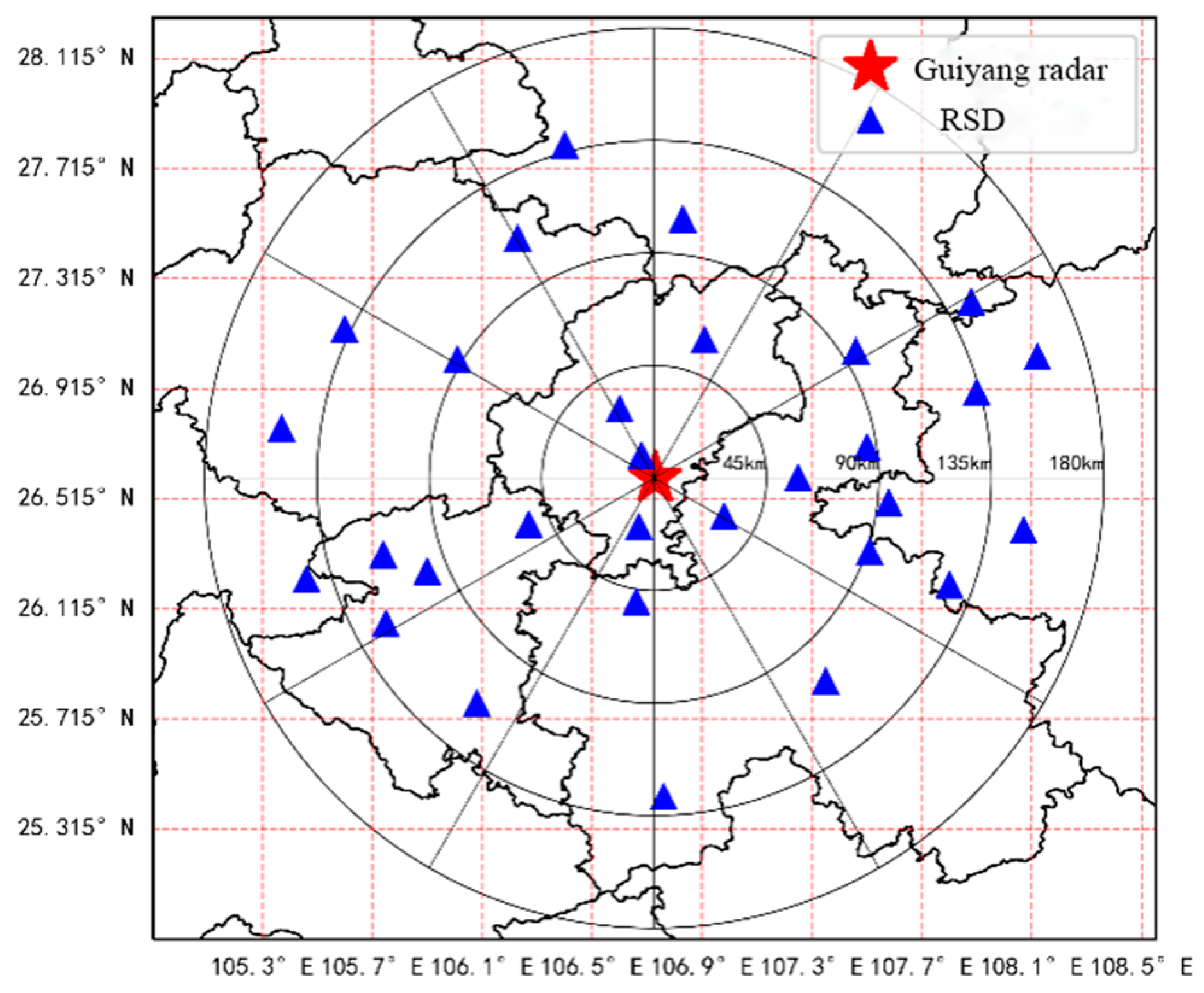
Guizhou Province is located in the east of the Yunnan-Guizhou Plateau in southwest China. The terrain in Guizhou Province is high in the west and low in the east, which slopes from the middle to the east, south and north, with an average altitude of about 1100 m. Its landforms are mainly of plateau mountains, hills, and basins, of which the mountain and hilly types account for 92.5% of the total area. It is reflecting the complex geomorphology of Guizhou Province and high-frequency precipitation characteristics. Therefore, this paper selects the circle research area centered at Guiyang radar with the radius of 150 km, where the radar detection data quality in this range is high and the RSD site is evenly distributed. The OTT-Parsivel disdrometer is used in this paper, which is an instrument for optical measurement of RSD based on modern laser technology, and the weather radar is a new generation of Doppler weather radar (CINRADCD). The topographic map and the distribution of RSD stations and radar stations in the study area are shown in Figure 1.
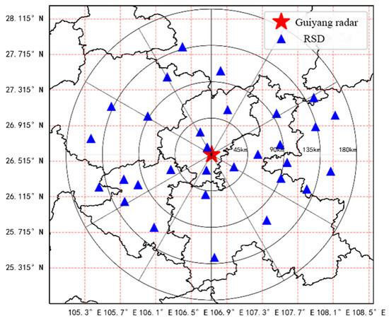
Figure 1.
Study area radar and RSD site distribution.
The OTT-Parsivel disdrometer measures particle sizes from 0.2 mm to 5 mm for liquid precipitation types and 0.2 mm to 25 mm solid precipitation types, and can measure precipitation particles at speeds from 0.2 to 20 m/s. It classifies the measured particles in two dimensions of diameter (D) and velocity (V), with 32 intervals set in each, resulting in a total of 32 × 32 = 1024 particle types. In addition, the disdrometer stores the retrieved precipitation intensity, retrieved radar reflectance sensor status, and original particle species data as binary data files every 5 min.
CINRAD/CD type new generation Doppler weather radar has the following specifications, wavelength range 1.5–3.75 m, frequency range 4000–8000 MHz, beam width of about 1 °, reflectivity factor distance resolution of 250 m, maximum detection distance of 250 km. The radar common body sweep mode is VCP21, that is, a body scan can scan 9 elevation angles in 6 min, the elevation angles are 0.5°, 1.5°, 2.4°, 3.4°, 4.3°, 6.0°, 9.9°, 14.6°, and 19.5°. 2 Analysis of raindrop spectrum characteristics of precipitation 2.0 Sketch out
Raindrop size distribution plays a crucial role in the study of microphysical precipitation processes because it has a profound impact on precipitation formation, the evolution of precipitation processes, and the quantitative estimation of precipitation by weather radar. In this paper, the data of RSD in Guizhou Province from March to September in 2020 are used to analyze the difference of RSD under different geographical situation, and to provide basis of data selection for the subsequent precipitation prediction with the use of the neural networks. Table 1 shows the basic information of the selected RSD stations. All three stations characterize by the subtropical monsoon humid climate, and the mountainous topography and landforms. Three stations with different altitudes are selected to study the influence of altitude on precipitation particle spectrum distribution through statistical analysis of data samples.

Table 1.
Basic information of RSD site.
In order to study the differences in the distribution of raindrop spectra in different geographical backgrounds, analyze the influence of altitude on the distribution of precipitation particle spectra, and provide data selection basis for neural network prediction of precipitation models. This study selected observation data from three different altitude raindrop spectrometer stations, namely Dafang, Majiang, and Luodian. Table 1 shows the basic information of the selected raindrop spectrometer stations.
Selecting the new generation Doppler weather radar (CINRAD/CD type) with a time resolution of 6 min from March to September 2020 in Guiyang, as well as the OTT Parsivel raindrop spectrum and rain gauge with a time resolution of 1 min from Dafang, Majiang, and Luodian stations. The three-sources data mainly considered the matching of weather radar and raindrop spectrometer in space. There is a strong correlation between weather radar detection data and precipitation data from the first 6 min in terms of time. Based on the radar data with the lowest time resolution, the raindrop spectrometer and automatic rain gauge data are reorganized according to the first 6 min of radar time to ensure that each sample of the three-sources data contains the same time to complete time matching.
2.1. Spectral Parameter Calculation
2.1.1. Data Quality and Methods
Particle density N(D) represents the total number of raindrop particles per unit volume, with the unit m−3 mm−1, and is calculated as follows,
where nij represents the number of particles in i-th diameter bin and the number of particles in the j-th velocity bin; A is the sampling base area of RSD, equalling to 5400 mm2; is the sampling time 60 s; Vj is the velocity value of the sampled particle in m/s.
2.1.2. Radar Reflectivity Factor
The radar reflectance factor, in mm6/m3, is calculated as follows,
2.1.3. Precipitation Intensity
The precipitation intensity is the precipitation per unit time, with the unit mm/h. The calculation formula is as follows,
where Di represents the diameter of the sampled particle, N(Di) is the number of particles at the current particle diameter and particle velocity [16].
2.1.4. Average Diameter
The average diameter is the sum of the diameters of all raindrops divided by the total number of raindrops, which is calculated as follows,
2.1.5. Mass-Weighted Average Diameter
The mass-weighted average diameter is the average diameter of the diameter weighted mass of all particles in a unit volume relative to the total mass of particles, in mm, and the calculation formula is as follows,
2.1.6. Average Volume Diameter
The average volume diameter represents the diameter of an equivalent raindrop whose volume is equal to the average raindrop volume, in mm, and is calculated as follows,
2.1.7. M-P Distribution and GAMMA Distribution
M-P distribution, which can be used to describe the spectral distribution of raindrops using an exponential function, is calculated as follows,
where the particle number density parameter N0 is in mm−1 m−3, and the particle scale parameter is in mm−1 [17].
In order to describe the RSD more accurately, Ulbrich proposed a method based on the M-P distribution to treat the RSD as a GAMMA distribution, and the calculation formula is as follows,
where the form factor is a dimensionless parameter. The function curve is curved upwards when . The function curve is curved downwards when [18]. The formula becomes an M-P distribution when .
2.2. Raindrop Size Distribution Analysis
2.2.1. Particles Are Distributed and Proportion
In Figure 2, the x-axis represents the particle size, with the unit mm. The y-axis represents the final falling velocity of the particle, in m/s. The color scale represents the particle number density in units. And it is arranged from top to bottom in descending order of site altitude, and the results shown are the average data of RSD inversion from March to August in 2020. The following conclusions are drawn from the figure, first, the particle distributions of three stations are similar, showing that the particles are concentrated in the smaller particle size range with the peak value being 0.312 mm. Second, the final falling velocity of raindrops is almost the same and its mainly distributed in the range of 1–5 m/s; Third, the particle number density spectrum width increases with the decrease of altitude.
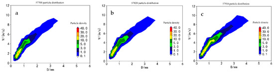
Figure 2.
Particle distribution (a) Dafang (57708) Station, (b) Majiang (57828) Station, (c) Luodian (57916) Station.
2.2.2. Particle Number Density and Proportion of Precipitation Intensity
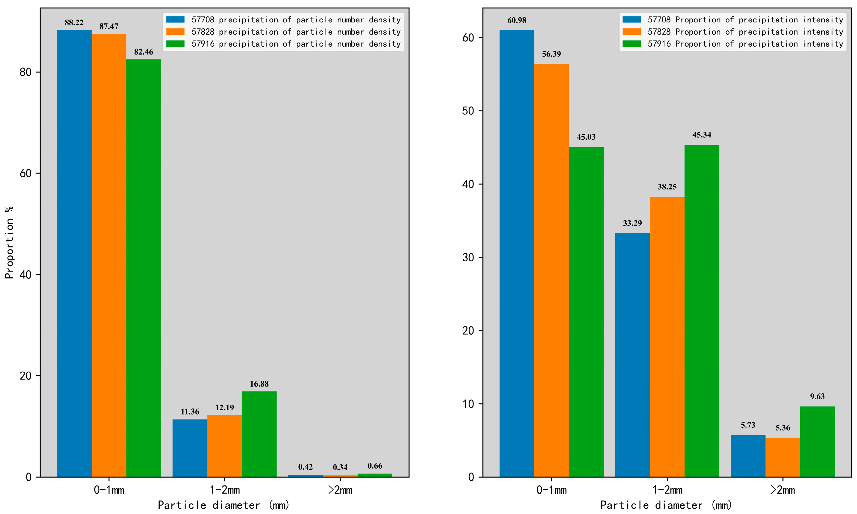
Here, the sample of RSD is divided in to three ranges (D < 1 mm, 1 < D < 2 mm, D > 2 mm) according to the particle size, then Statistical analyses are performed separately. As shown in Figure 3, small raindrops are an important component of the size spectrum in the three stations. With the decrease of altitude, the ratioproportion of small particle over total particles decreases, while the number of large size particles increases. The key reason may be that the collision and growth process of raindrops during the falling process. consumes those small-sized particles and increases the concentration of those large-sized particles. Moreover, in terms of precipitation contribution rate, in Dafang (57708) station and Majang (57828) station, the precipitation intensity are mainly provided by small size particles. While particles larger than 1 mm particle size can provide a higher precipitation intensity with need to only a lower particle number density, which is caused by the sensitivity of precipitation.
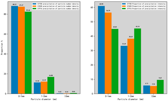
Figure 3.
Particle density and intensity proportion precipitation intensity.
2.2.3. Z-I Relationship
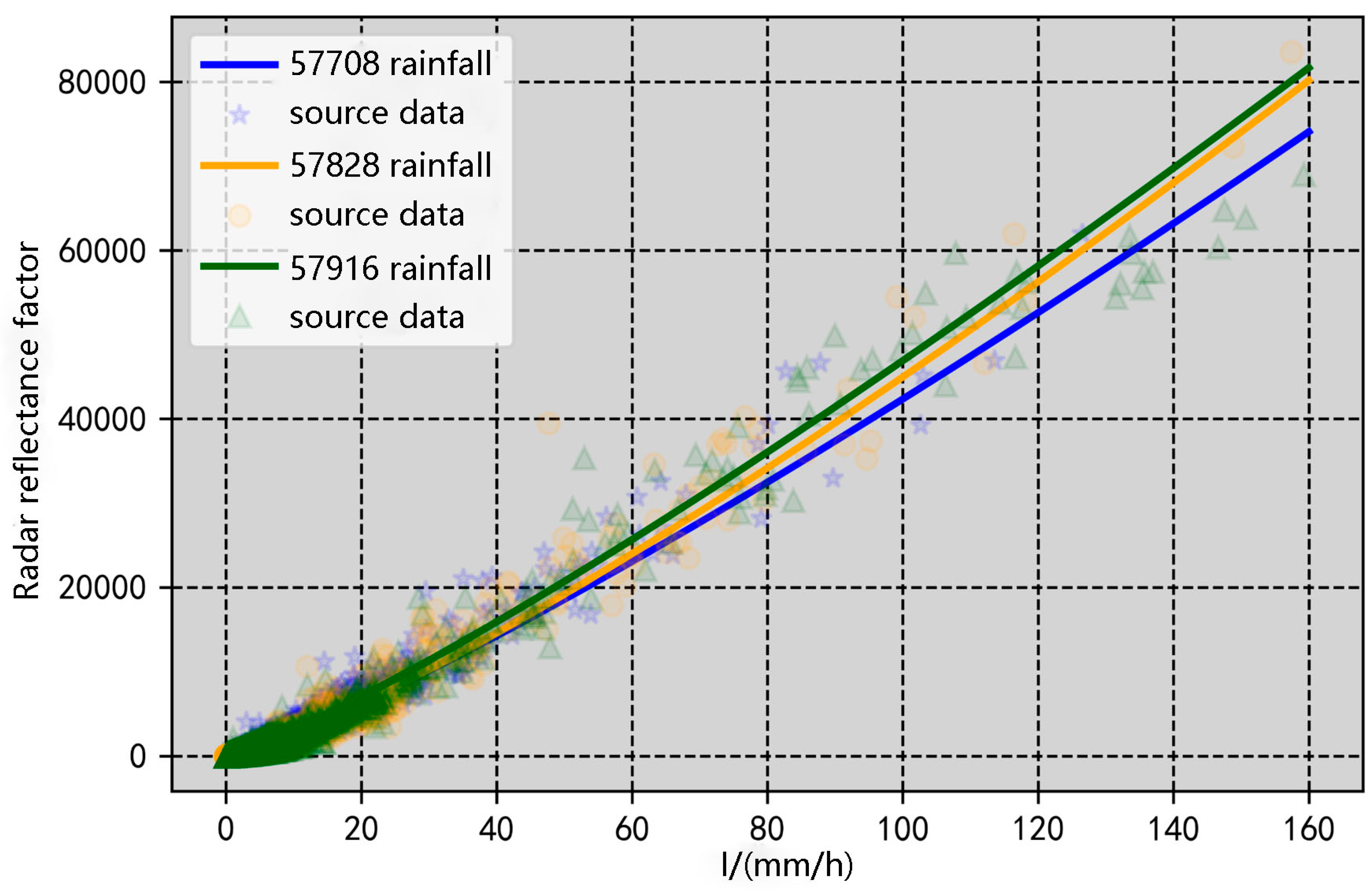
The source data shown in Figure 4 are the precipitation samples from March to September in 2020 at the three stations, and the curve is the fitting result of source data using the least square method. The site fitting curve of Dafang (57708) is , the fitting curve of Majiang (57828) station is , and the fitting curve of Luodian (57916) station is . Compared with the classical radar quantitative precipitation estimation curve , the coefficient values are quite different. If the classical Z-I curve is used for precipitation estimation, the precipitation will be underestimated to a certain extent under the same radar reflectance factor.

Figure 4.
Z-I diagram intensity to particle diameter.
2.2.4. Raindrop Size Distribution Fitting
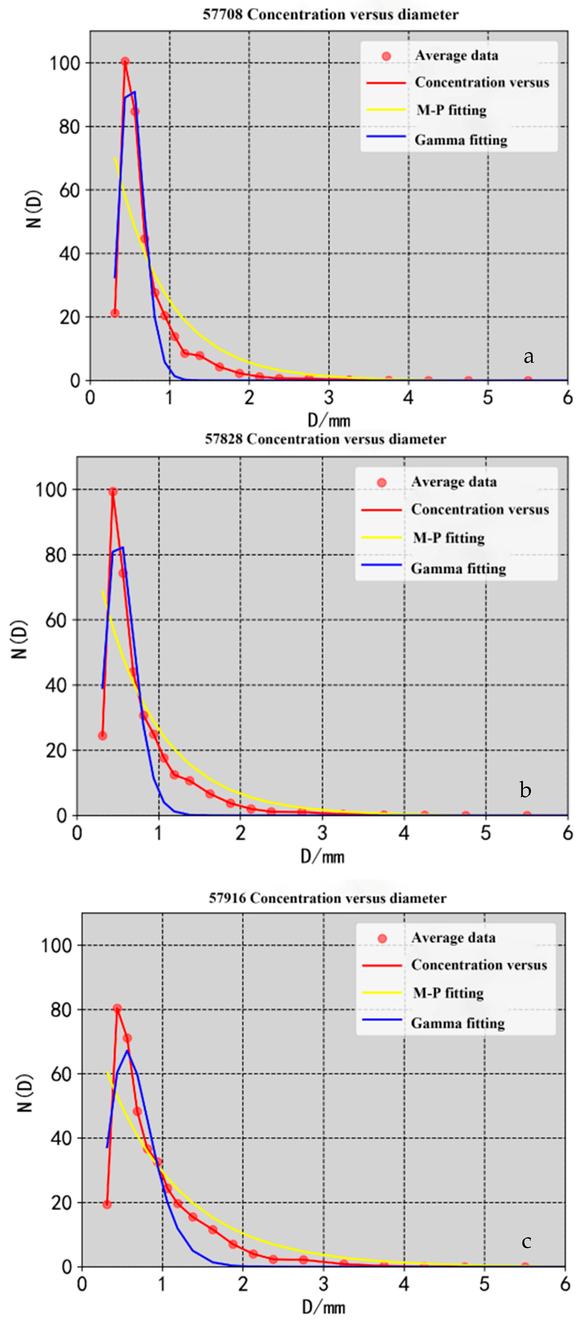
Figure 5 are the fitting curves of the M-P and GAMMA distribution by using the least squares method, in which the x-axis represents the particle diameter and the y-axis represents the particle number density. Furthermore, the data sample is the precipitation base data of the three stations from March to September in 2020, and the distribution of precipitation particles in the rainfall process of the three places is analyzed by the average particle density spectrum. It can be seen from Figure 5 that the precipitation particle spectra of the three places are unimodal, with a peak of 0.312 mm. In addition, the raindrop spectra of Dafang (57708) station with a higher altitude have a higher particle concentration of small particle size (D < 1 mm), while Luodian (57916) station with a lower altitude occupies a higher particle concentration in a different size bin (1 < D < 3 mm).

Figure 5.
Average RSD, M-P distribution and Gamma distribution fitting ((a) Dafang (57708) Station (b) Majiang (57828) Station (c) Luodian (57916) Station).
2.2.5. Particle Diameter Fitting
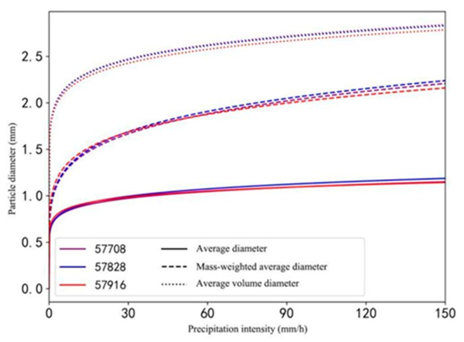
In Figure 6, the x-axis represents the precipitation intensity (PI), the y-axis represents the precipitation particle diameter, and the simulated value of PI ranges from 0 to 150 mm/h. The following conclusions are drawn from the figure, first, the fitting curve of the average diameter of rainfall in the three stations in 2020 has a small variation with the increase in rain intensity. And only has significant changes when the PI is low, and basically maintains around 1 mm without much fluctuation in the area with large PI. Second, the average diameter is the lowest of the three diameters in the range of the simulated value of PI; the mass-weighted average diameter and average volume diameter fit curve amplitude are larger, where the average of the latter is relatively larger than that of the former.
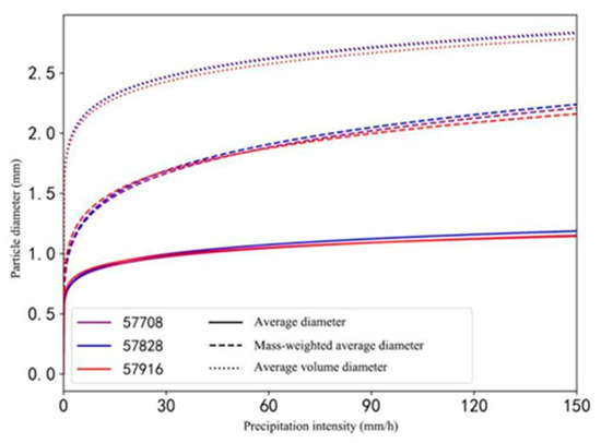
Figure 6.
Fitting relation of particle diameter (57708, 57828, 57916).
Figure 7 shows a precipitation process in June at Dafang (57708) station. During the early and late precipitation periods where the precipitation intensity remains low, the two curves coincide with each other. But when the precipitation intensity is high, the performance of the average volume diameter is significantly stronger than that of the mass-weighted average diameter. According to the calculation, the correlation coefficients between the mass-weighted average diameter, and the average volume diameter and the precipitation intensity are 54.84% and 69.15%, respectively, indicating that the average volume diameter has a stronger correlation with the precipitation intensity.
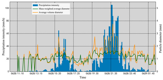
Figure 7.
Mass-weighted average diameter and average volume diameter change with precipitation intensity.
Based on the comparative analysis of the particle distribution and microphysical characteristic parameters of the rainfall process mentioned above, it can be concluded that in the precipitation process of the three stations, first, the particle landing velocity distribution is very similar. Second, the particle size less than 1 mm contributes the most to the particle density and decreases with the descending altitude. Third, the GAMMA distribution fit effect is better in the two distribution fittings, and average volume diameter than mass-weighted average diameter fit better with variation in precipitation intensity.
3. Neural Networks Predict Precipitation
3.1. Predicting Neural Network Configuration
3.1.1. Prediction Network Structure
Based on the data of Guiyang weather radar, Dafang station raindrop spectrometer, and automatic rain gauge, an LSTM neural network method was applied to construct a precipitation prediction model for Guizhou. The start and end times of the data are shown in Table 2.
Table 2.
Data Overview.
The prediction model adopts two independent LSTM neural networks, in which the predicted values of precipitation and benchmark are given by prediction and benchmark network. The actual prediction value is obtained by subtracting the output value of the prediction network and the benchmark network, which the basic structure of the network is shown in Figure 8.
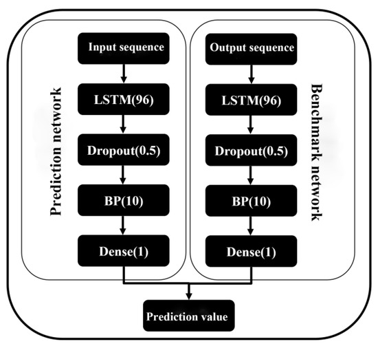
Figure 8.
The basic structure of prediction neural network.
Firstly, the source data are fed into the LSTM layer for training. Then the Dropout layer randomly discards half of the connected neurons to increase the network generalization ability. Finally, output the training results through the BP layer and the single neuron Dense layer without activation function.
3.1.2. Prediction Dataset Construction
Neural network training requires feature values and prediction values, where the former is the input that the neural network needs to learn and the latter is the output that calculated by the neural network after a series of changes in the weight coefficients. In this experiment, the selection of features first takes into account the physical quantities with a strong correlation with precipitation intensity in the inversion parameters of the RSD, which can be obtained from Equation (3). The particle diameter, particle fall velocity and particle number density parameters are selected here as the input values due to the usage in the precipitation intensity inversion of the RSD. In terms of radar reflectance intensity, considering the distance between the RSD site and the radar station, the data in the 1–3 layers body sweep are selected as the feature input. Since the data of the rain gauge are usually regarded as the true values from the precipitation measuring, they are selected as the true value here. The parameters used in our research are shown in Table 3, and the prediction values are measured by rain gauges.
Table 3.
Estimation of neural network inputs.
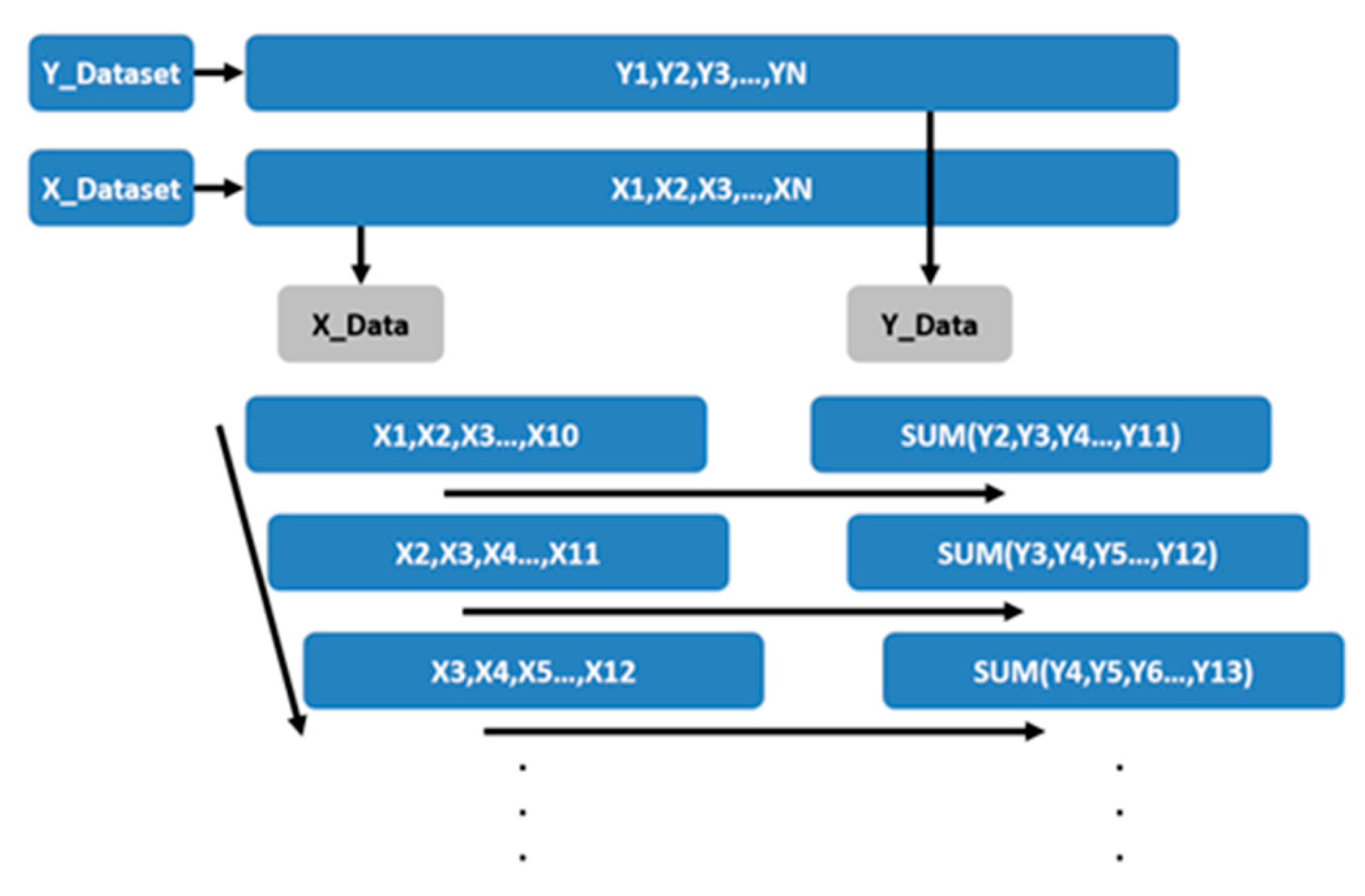
If the prediction values were ahead time of the feature values, the neural network is for precipitation prediction. After the data of the tipping bucket rain gauge, RSD and weather radar are matched in time and space, their projections on the ground coincide. The start time and end time of the corresponding samples are the same, of which the RSD and weather radar data are used as feature values, with the tipping bucket rain gauge data as the predictive value. The prediction dataset is constructed as shown in Figure 9.

Figure 9.
Predictive dataset construction.
In Figure 9 X-Dataset represents the sequences set of the feature values, and Y-Dataset represents the sequences set of the prediction values, in which X1, X2, X3…XN corresponds to Y1, Y2, Y3…YN. And the input dataset of the neural network is constructed based on two datasets above. Since precipitation is a continuous process in time and the intensity is also continuously changed. When constructing the dataset need to consider the input feature values to form a continuous time series. However, the prediction value considering the convergence speed and training accuracy of the neural network uses the accumulation of the time series as the input.
In Figure 9, X-Data and Y-Data are the input data sets of the neural network. Firstly, in the first row of the first column of data, X-Data takes X1 to X10 as the features. In the second column of the first row, Y-Data takes the sum of Y2 to Y11 as the prediction value. The starting time of prediction value accumulation intervals is ahead of the feature value for one radar body sweep time. Therefore, this set of data is the input of the first 10 radar sweep time to predict the rainfall after 1 radar sweep time. Similarly, for the purpose of prediction after N radar body sweep times, X-Data remains unchanged and Y-Data only need to move the starting point for N times. Secondly, taking the sample count into account, it can be seen in the vertical direction of the block diagram that the starting point of each group is shifted back one sample time in turn, so that the time resolution of the constructed sample will be a single radar body sweep time. The dataset constructed by sliding at this time resolution can not only maximize the use of samples, but also improve the ability of neural networks to calculate the start and stop of precipitation. Although the two neural network structures are the same, there are differences in the input sequence. Where the X-Data of the input are the same, but the input Y-Data are different, as shown in Figure 10.
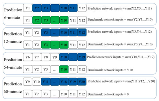
Figure 10.
Prediction network and benchmark network inputs.
In Figure 10, the prediction input of the prediction network keeps the accumulation of the 10-time body scan data unchanged, and slides for one body scan time sequentially along the time axis according to the prediction time. The prediction value of the benchmark network remains unchanged at the last one Y10, and the starting time is moved back along the time axis by 1 time according to the prediction time. The method of subtracting the training results from the prediction network and the benchmark network has the following advantages over the method of direct prediction, (1) The use of dual network training can reduce the systematic error in the training process. (2) Compared with direct prediction, the dual network is more accurate in predicting within 60 min. (3) Parameter configuration.
Neural network training is a very complex process. With the increase of network depth, neurons, feature values and other factors, activation function, network hyperparameters to the neural network convergence speed and training accuracy is crucial. And some of the parameters in the LSTM network as shown in Table 4.
Table 4.
LSTM network parameters.
3.2. Prediction Result Evaluation
3.2.1. Prediction of Convective Cloud Precipitation Process
A convective cloud precipitation event is selected on July 18, and the precipitation forecasts of 6 min, 18 min, 30 min, 60 min, 90 min and 120 min are carried out at the Dafang (57708) station, with the precipitation process began at 21,05 on 18 July 2020 lasting about 7 h from that time on. In this case the precipitation is 37.3 mm, the precipitation intensity inverted by RSD peaked with the value being 26.78 mm/h.
Table 5 was the evaluation index of neural network precipitation prediction, and it can be seen from the table that the real-time correlation coefficient and the optimal average relative error of the prediction 60-min network in the prediction time point reaches 0.9287 and 0.3897, respectively. The real-time prediction with time resolution more than 60 min is the same. Besides, the 60-min prediction index is better than the 90-min and 120-min forecast as a whole. In the 60-min prediction the good performance of the real-time correlation coefficient and the mean relative error indicates that it has a better performance in predicting the precipitation trend and the precipitation intensity consistency compared with other times.
Table 5.
Prediction and evaluation index of neural network of convective cloud precipitation process.
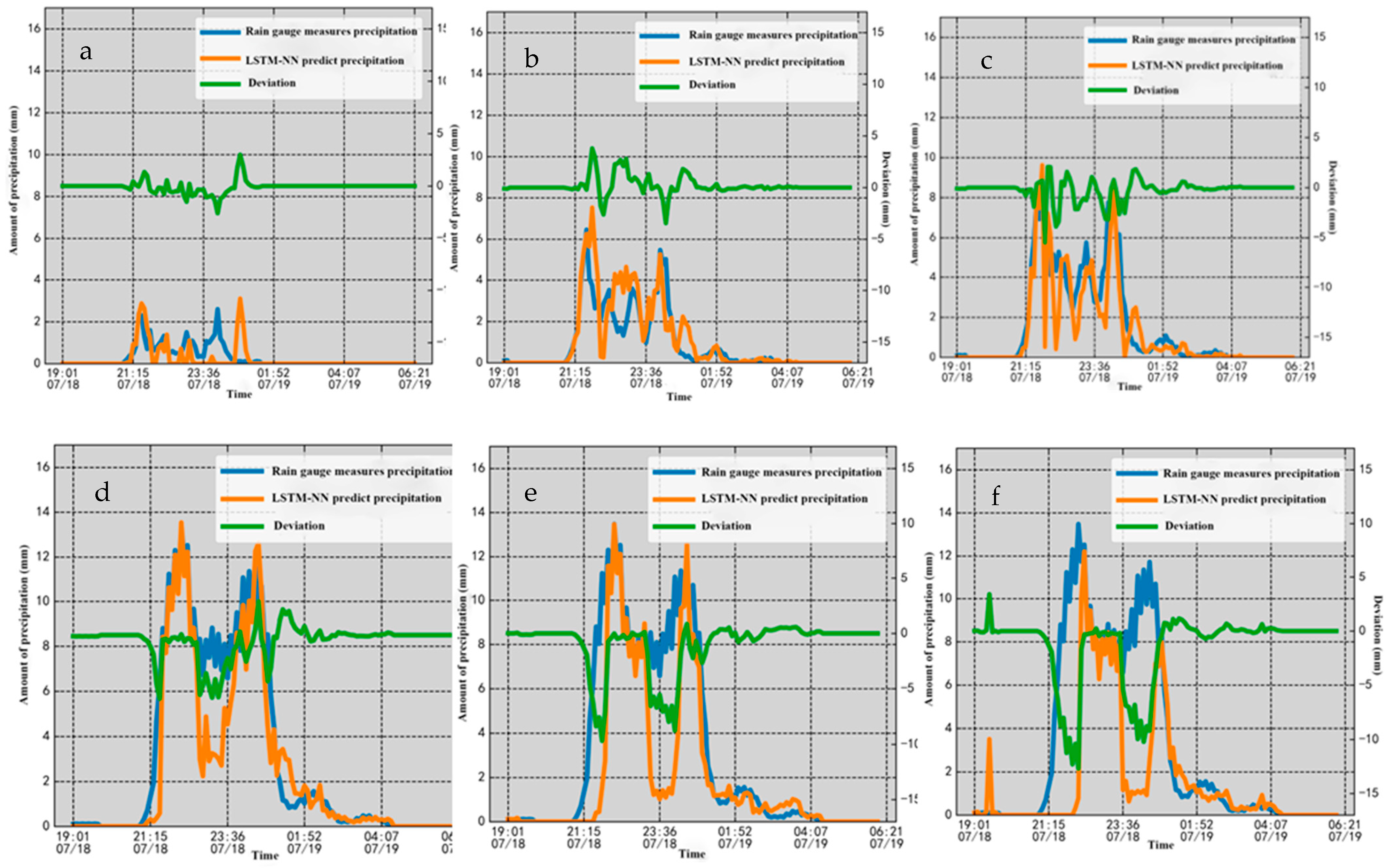
Figure 11 shows that the deviation at the beginning of the two precipitations always tends to be negative, indicating that the prediction value is underestimated compared to the rain gauge detection value. That is, the rain gauge detects precipitation earlier than the neural network. Due to the principle and characteristics of the detection instrument, the neural network input feature parameter can capture the precipitation information of the priority rain gauge, but sometimes the rain doesn’t exist near the measurement area at all. That’s because the neural network input can only determine the occurrence of precipitation when there is enough precipitation information. If the actual raining time is short, the neural network can ignore the precipitation process easily.

Figure 11.
Real-time prediction of convective cloud precipitation process by neural network ((a) 6 min, (b)18 min, (c) 30 min, (d) 60 min, (e) 90 min, (f) 120 min).
There is a significant difference between the rain gauge and the neural network prediction of rainfall during the precipitation process. The real-time correlation coefficient reflects the gap between the neural network’s real-time rainfall prediction and the rain gauge detection result, which can be reflected in the time mismatch and numerical gap. Since the prediction is using the data of the first 1 h to predict the future time. When the precipitation intensity changes drastically and the input feature value of the neural network has not yet received the change, but the ground rain gauge detection data will be reflected anyway, which causes a time mismatch, and it becomes more obvious as the predicted time increases. In order to find the cause of the numerical difference, the relationship between the features of the network model and the prediction values is found after controlling the variables, (1) Radar reflectance is mainly used to determine the start and end time of precipitation, and auxiliary revision of predicted precipitation intensity. (2) The average velocity mainly plays an auxiliary role in revising the predicted precipitation intensity and has little influence on the results. (3) The predicted precipitation intensity is mainly affected by the combined effect of average volume diameter and particle number density. The average volume diameter has a high weight on the amplitude of predicted precipitation intensity, and particle number density has a great influence on the fluctuation of predicted precipitation, so single value cannot predict precipitation well. Although the rain gauge and the RSD are geographically similar coincident, it can be seen that the prediction values have a strong correlation with the current precipitation structure. However, the surface measurement data of the two instruments does not coincide with each other, the time series of the data cannot be completely consistent, which is also an important reason for the difference of real-time numerical prediction.
Although the neural network on the real-time precipitation is different from the rain gauge, this error will be compensated before and after the time point. If the time series is stretched or predicted the total rainfall process, the predicted result of the neural network will be closer to the actual precipitation.
3.2.2. Prediction of Stratiform Cloud Precipitation Process
A continuous stratiform cloud precipitation weather on July 19 is also selected, and the precipitation forecasts of 6 min, 18 min, 30 min, 60 min, 90 min and 120 min are carried out at the Dafang (57708) station. The precipitation began at 17,36 on July 19, 2020 lasting about 7 h. The precipitation is 6.7 mm and the RSD inverted precipitation intensity comes with a peak of 4.98 mm/h.
Table 6 was the neural network precipitation evaluation prediction index. From the Table 5 it can be obtained that the characteristics of the stratiform cloud precipitation evaluation index are basically the same as the convective cloud precipitation. Besides, the real-time correlation coefficient and the average relative error are the best prediction results of 60 min, reaching 0.9357 and 0.3312 respectively. It can be concluded that the prediction 60 min neural networks have strong predictive ability for weak precipitation process. It can also be seen from Figure 12 that as the forecast time increases, the rain gauge detection data tends to smooth out, and the neural network prediction effect continues to improve. This is due to the fact that the rain gauge detection process in the weak precipitation process is greatly affected by the tipping bucket residual error, which itself has a certain deviation from the actual weather phenomenon, and the increase in the predicted time of the neural network can weaken this deviation to a certain extent. And we see that there is no lag error in stratiform precipitation as there is in convective precipitation. After checking the data set, it is found that the weather radar and RSD detected from the precipitation information long before the rain gauge, because the echo was developed over the area. If the precipitation due to echo motion occurs during the convective cloud precipitation process, the weather radar will detect the echo of the earlier rain gauge at one or two individual sweep time, and the phenomenon of prediction lag will be easy to occur when the it is detected by time. Finally, in terms of the RSD, the relatively weak precipitation information can be captured by the higher detection accuracy, and the more complete precipitation process can be obtained for the precipitation with stable development.
Table 6.
Prediction and evaluation index of neural network of stratiform cloud precipitation process.
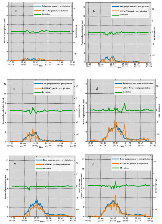
Figure 12.
Real-time prediction of stratiform cloud precipitation process by neural network ((a) 6 min (b) 18 min (c) 30 min (d) 60 min (e) 90 min (f) 120 min).
4. Conclusions
In this paper, the base data of the new generation Doppler weather radar (C-band) in Guizhou Province, the raw data of the OTT-Parsivel laser RSD and the precipitation data of the automatic meteorological observation station are used. Three RSD stations are selected for RSD analysis according to the difference in altitude, then the three-source data are used to predict the precipitation through the LSTM neural network. The conclusions of the study are as follows,
(1) From the distribution characteristics of RSD in Dafang (57708) station, Majang (57828) station, and Luodian (57916) station (with an altitude of 1722.7 m, 985.0 m, and 441.5 m, respectively) in Guizhou, we can conclude that the particle size of less than 1 mm contributes the highest to the density of particle numbers, reaching 88.22% and decrease with the descending altitude. In addition, in the fitting of RSD, the GAMMA distribution fit has more advantages than the M-P distribution fit in the small particle size region (D1 mm), while the M-P distribution fit is more accurate in the large particle size region. In general, the GAMMA distribution fit effect is better, and increases with the ascending altitude. Finally, in terms of the correlation between particle size and precipitation intensity, the mass-weighted average diameter is not sensitive enough to the response to the change of precipitation intensity, but the correlation between the average volume diameter and the precipitation intensity is higher, with correlation coefficients being 54.84% and 69.15%, respectively.
(2) In terms of precipitation prediction, in the process of convective cloud precipitation the 60 min forecast index is better than the 90, 120 min forecast. Although the real-time precipitation neural network has an obvious difference from the rain gauge, this error will be compensated before and after the time point. If the time series is elongated or predict the total rainfall of a process, the prediction results of the neural network will be closer to the actual precipitation. Similarly, in the process of stratiform cloud precipitation, it is shown that the prediction 60-min neural network has behaves better for the weak precipitation prediction. The detection data tends to be smooth and the predicted effect of the neural network continues to improve with the increase of prediction time. In conclusion, in the prediction of convective cloud and stratiform cloud precipitation process the 60-min prediction results have the highest consistency with the actual precipitation, and the correlation coefficients can reach 0.9287 and 0.9257, respectively.
Author Contributions
Methodology, X.A.; software, X.A.; validation, Q.W.; investigation, F.W.; resources, F.W.; data curation, Z.L. and L.H.; supervision, D.S.; funding acquisition, D.S. All authors have read and agreed to the published version of the manuscript.
Funding
This work was supported by the Sichuan Provincial Natural Science Foundation (2022NSFSC0208) and the Open Fund Project of the Key Laboratory of Land Surface Processes and Climate Change in Cold and Arid Regions, Chinese Academy of Sciences (LPCC2020009) and Project of Introducing Talents for Scientific Research, KYTZ2023034. The National Science Foundation of Sichuan Province (No. 2022NSFSC1006).
Institutional Review Board Statement
Not applicable.
Informed Consent Statement
Not applicable.
Data Availability Statement
The data presented in this study are available on request from the corresponding author. The data are not publicly available due to privacy.
Conflicts of Interest
The authors declare no conflicts of interest.
References
- Wu, J.-S.; Jin, L.; Nong, J.-F. Forecast Research and Applying of BP Neural Network Based on Genetic Algorithms. Math. Pract. Theory 2021, 47, 843–853. [Google Scholar]
- Huang, X.; Yin, J.; Ma, L.; Huang, Z. Comprehensive Statistical Analysis of Rain Drop Size Distribution Parameters and Their Application to Weather Radar Measurement in Nanjing. Atmos. Sci. 2019, 43, 691–704. [Google Scholar]
- Lin, H.-B.; You, Q.-L.; Jiao, Y.; Min, J.-Z. Spatial and Temporal Characteristics of the Precipitation over the Tibetan Plateau from 1961 to 2010 Based on High Resolution Grid-observation Dataset. J. Nat. Resour. 2015, 30, 271–281. [Google Scholar]
- Shen, G.; Gao, A.; Li, J. Application of Raindrop Spectrum and Dual Polarization Radar Data to a Heavy Rain Process. Meteorological 2021, 47, 737–745. [Google Scholar]
- Cai, Z.; Liu, J.; Liao, A.; Liao, M.; Liu, H.; Wang, H.; Ma, T.; Zhuo, P. Analysis of characteristics of raindrops based on distrometers. J. Adv. Sci. Technol. Water Resour. 2021, 41, 93–98. [Google Scholar]
- Zeng, G.; Guo, Z.; Zhou, Q.; Zhang, H.; Chen, X.; Guo, J. Application evaluation of dual polarization radar quantitative precipitation estimation algorithm based on laser raindrop spectrum. Meteorol. Res. Appl. 2021, 42, 95–100. [Google Scholar]
- Zea, L.R.; Nesbitt, S.W.; Ladino, A.; Hardin, J.C.; Varble, A. Raindrop Size Spectrum in Deep Convective Regions of the Americas. Atmosphere 2021, 12, 979. [Google Scholar] [CrossRef]
- Mercier, F.; Chazottes, A.; Barthès, L.; Mallet, C. 4-D-VAR assimilation of disdrometer data and radar spectral reflectivities for raindrop size distribution and vertical wind retrievals. Atmos. Meas. Tech. 2016, 9, 3145–3163. [Google Scholar] [CrossRef]
- Zhu, P.; Li, S.; Xiao, J.; Xu, L.; Jin, S. Study on Extrapolation Technique of Weather Radar Echo and lts Application to Nowcasting. Meteorological 2008, 34, 3–9. [Google Scholar]
- Liu, G.; Tang, Y.; Ban, R.; Lu, X.; Deng, R.; Huang, F.; Yang, Y. Brief Discuss on the conceptual model forecasting tool of the Maximum and minimum temperatures Sudden change. Meteorol. Res. Appl. 2009, 30, 22–24+108. [Google Scholar]
- Cheng, C.; Chen, M.; Wang, J.; Cao, F.; Yang, H. Short-term quantitative precipitation forecastexperiments based on blending of nowcasting with numerical weather prediction. Acta Meteorol. Sin. 2013, 71, 397–415. [Google Scholar]
- Elshaboury, N.; Elshourbagy, M.; Al-Sakkaf, A.; Abdelkader, E.M. Rainfall forecasting in arid regions using an ensemble of artificial neural networks. J. Phys. Conf. Ser. 2021, 1900, 012015. [Google Scholar] [CrossRef]
- Sharadqah, S.; Mansour, A.M.; Obeidat, M.A.; Marbello, R.; Perez, S.M. Nonlinear Rainfall Yearly Prediction based on Autoregressive Artificial Neural Networks Model in Central Jordan using Data Records, 1938–2018. Int. J. Adv. Comput. Sci. Appl. 2021, 12, 240–247. [Google Scholar] [CrossRef]
- Gunathilake, M.B.; Senerath, T.; Rathnayake, U. Artificial neural network based PERSIANN data sets in evaluation of hydrologic utility of precipitation estimations in a tropical watershed of Sri Lanka. AIMS Geosci. 2021, 7, 478–489. [Google Scholar] [CrossRef]
- Zhang, S.; Wei, Z.-Y.; Zhang, Y.-B. Forecasting Rainfall with Recurrent Neural Network. Water-Sav. Irrig. 2017, 5, 63–66+71. [Google Scholar]
- Pruppacher, H.R.; Klett, J.D.; Wang, P.K. Microphysics of Clouds and Precipitation; Springer: Berlin/Heidelberg, Germany, 1998. [Google Scholar]
- Marshall, J.S.; Palmer, W.M.K. The Distribution of Raindrops with Size. J. Atmos. Sci. 1948, 5, 165–166. [Google Scholar] [CrossRef]
- Ulbrich, C.W. Natural variations in the analytical form of the raindrop size distribution. J. Clim. Appl. Meteorol. 1983, 22, 1764–1775. [Google Scholar] [CrossRef]


Disclaimer/Publisher’s Note: The statements, opinions and data contained in all publications are solely those of the individual author(s) and contributor(s) and not of MDPI and/or the editor(s). MDPI and/or the editor(s) disclaim responsibility for any injury to people or property resulting from any ideas, methods, instructions or products referred to in the content. |
© 2024 by the authors. Licensee MDPI, Basel, Switzerland. This article is an open access article distributed under the terms and conditions of the Creative Commons Attribution (CC BY) license (https://creativecommons.org/licenses/by/4.0/).