Review

Some Early Studies of Isotropic Turbulence: A Review

by
John Z. Shi
State Key Laboratory of Ocean Engineering, School of Ocean and Civil Engineering, Shanghai Jiao Tong University, 1954 Hua Shan Road, Shanghai 200030, China
Atmosphere 2024, 15(4), 494; https://doi.org/10.3390/atmos15040494
Submission received: 20 February 2024 / Revised: 11 April 2024 / Accepted: 14 April 2024 / Published: 17 April 2024
(This article belongs to the Special Issue Isotropic Turbulence: Recent Advances and Current Challenges)

Abstract

:
A re-examination of some early classic turbulence literature, mainly of isotropic turbulence, is given in this selective review. Some early studies, including original concepts and points, are reviewed or highlighted. Two earliest studies and six major original concepts are found: (i) Lord Kelvin’s pioneering elementary studies of homogeneous, isotropic turbulence; (ii) Kelvin’s early introduction of Fourier Principles into turbulence studies; (iii) the Kelvin elementary concept of the direct energy cascade; (iv) the Kelvin early concept of the symmetry of turbulence; (v) the Taylor concept of the coefficient of eddy viscosity; (vi) the Taylor concept of the ‘age’ of the eddy; (vii) the Taylor–Fage–Townend concept of small eddies or microturbulence or small scale turbulence; and (viii) the Obukhov concept of a function of the inner Reynolds number (i.e., R e dependent coefficient) in both the balance equation and the energy distribution equation (the two-thirds law). Both Kelvin and Taylor should be regarded as the co-founders of the statistical theory of homogeneous, isotropic turbulence. The notion, ‘the Maxwell–Reynolds decomposition of turbulent flow velocity’, should be used. The Kolmogorov–Obukhov scaling laws are reviewed in detail. Heisenberg’s inverse seventh power spectrum is briefly reviewed. The implications or significances of these early studies, original concepts and points are briefly discussed, with special reference to their possible links with modern approaches and theories.

1. Introduction

Great classics, when revisited in the light of new developments, may reveal hidden pearls,… (Frisch [1] 1995, page xi, Preface, lines 2–3).
What is turbulence? When did the scientific study of turbulence start? Is turbulence the same at different temporal and spatial scales or different? Does turbulence have any different types? Perhaps it is not so easy to give satisfactory answers to these questions. In the present author’s view, studies of turbulence can return to Saint-Venant [2] (1843) and Helmholtz’s [3] (1868) On discontinuous movements of fluids. Prandtl [4] (1938, page 340, paragraph 1, bottom) outlines four types of turbulence: (a) wall turbulence; (b) free turbulence; (c) turbulence in stratified flows; and (d) decaying isotropic turbulence. In some way, Prandtl might have stimulated Hinze’s [5] (1959, vii–viii) classification of turbulence as (i) isotropic turbulence; (ii) nonisotropic turbulence; (iii) nonisotropic free turbulence; and (iv) nonisotropic “wall” turbulence. Gence [6] (1983, page 202) discusses the general features of the following three types of homogeneous turbulence: (1) homogeneous and isotropic turbulence; (2) homogeneous and anisotropic turbulence without a mean velocity gradient; (3) homogeneous turbulence with a constant mean velocity gradient. Despite some developments having been made within the general field of turbulence, some of the simplest problems involving isotropic turbulence have still defied a full solution.
What is isotropic turbulence? As a simple example, Figure 1 shows the generation of isotropic turbulence by oscillating grids (5 cm × 5 cm) within a mixing box.
In the spirit of Osborne Reynolds’ experimental investigation, general early investigations or statistical measurements of (isotropic) turbulence were made by Taylor [7,8] (1914/1915, 1927e), Dryden and Kuethe [9] (1929), Mock and Dryden [10] (1932), Fage and Townend [11] (1932), and Townend [12] (1934). The statistical theory of isotropic turbulence, however, is generally thought to be initiated by Taylor [13,14,15,16,17,18,19] (1921, 1935c, 1935d, 1935e, 1935f, 1936d, 1937), experimentally investigated or verified by Simmons and Salter [20] (1934), Townend [12] (1934), Dryden [21] (1937), Dryden et al. [22] (1937), Prandtl [4] (1938), Simmons and Salter [23] (1938), Dryden [24] (1939), and further extended by others, e.g., von Kármán [25] (1937), de Kármán and Howarth [26] (1938), Robertson [27] (1940), Kolmogorov [28,29] (1941a, c), Millionschikov [30] (1941), Heisenberg [31,32] (1948a, b), Lin [33] (1948), and Chandrasekhar [34,35,36] (1949a, b, c). Extensive reviews of isotropic turbulence can be found in the literature (e.g., Dryden [37] 1943, Chandrasekhar [38] 1949d, Agostini and Bass [39] 1950, Batchelor [40] 1953, Chapter 3 in Hinze [5] 1959, Leslie [41] 1973, Monin and Yaglom [42,43] 1971, 1975, Gence [5] 1983, McComb [44,45] 1990, 1995, Sreenivasan and Antonia [46] 1997, Moffatt [47] 2012, McComb [48] 2014, Shi [49,50] 2021a, b). Recently, Panickacheril et al. [51] (2022) presented a review of numerical simulations that considers the collection of past studies of the decay of homogeneous and isotropic turbulence.
Considering the extensive studies and reviews of isotropic turbulence available in the literature, are there any more points left that can make a review worthwhile? What is it that motivates the present author to write this review? On a personal note, after the publications of his own two reviews (Shi [49,50] 2021a, b), the present author found that some original concepts and points were missing in those reviews. It may be the appropriate time to present them in this Special Issue. It is hoped that this selective review can be complementary to Professor David McComb’s Editorial in this Special Issue on isotropic turbulence.
The general motivation for writing the article is to show how the idea of turbulence developed from a simple laminar flow to a rather complex spectral analysis of energy density. This article attempts to provide an overview, starting with the early work of Lord Kelvin and ending with the work of Kolmogorov, Obukhov, Heisenberg, and Chandrasekhar, and some insight into the evolution of the concept of homogeneous isotropic turbulence.
The primary objective of this review is to re-examine some selective classical literature about isotropic turbulence in order to further the details of some early concepts and points which might be missing in the literature. Focus is also placed on their possible links with modern approaches and theories. The overall structures of the remainder of this review are as follows: Section 2 highlights the gradient transport hypothesis or eddy viscosity by Saint-Venant and Boussinesq. Section 3 briefly reviews James Thomson’s laminar theory of the flow in rivers and other open channels. Section 4 gives a detailed account of Kelvin’s contributions to the mathematical and physical studies of homogeneous, isotropic turbulence. Section 5 highlights the Maxwell–Reynolds decomposition of turbulent flow velocity. Section 6 re-examines the early ideas of the Taylor statistical theory of isotropic turbulence. Section 7 presents a revisit to the Kolmogorov–Obukhov scaling laws. Section 8 discusses the Heisenberg statistical theory of homogeneous, isotropic turbulence. Section 9 discusses the implications or significance of those early studies, original concepts, and points. Finally, the Conclusions are presented in Section 10.

2. The Remarkable Work of Saint-Venant and Boussinesq on Turbulence

On the one hand, to place this review within the general context of a brief history of turbulence as much as possible; on the other hand, to provide a possible historical background to James Thomson’s Laminar Theory in Section 3, this section gives a short historical account of Saint-Venant’s [2] (1843) and Boussinesq’s [52] (1877) early contributions to the notion of gradient transport hypothesis or eddy viscosity. Although their remarkable work on turbulence is already presented in Frisch [1] (1995), the present author feels that some further details can still be added. To be consistent with Frisch’s [1] review, the title of this section is taken from Frisch [1] (1995). Note that Saint-Venant [2] (1843) and Boussinesq [52] (1877) can be easily found online but are generally not so easy to understand since they are old French writings/presentations.
The concept of eddy viscosity has been attributed to Saint-Venant and Boussinesq, as highlighted in Frisch [1] (1995). In the meantime, the notion of gradient transport hypothesis or eddy viscosity is evident in Saint-Venant [2] (1843) and Boussinesq [52] (1877). In addition, the mathematical expression of gradient transport or eddy viscosity is presented in Saint-Venant [2] (1843) and Boussinesq [52] (1877). As shown in Figure 2, Equation (3) in Saint-Venant [2] (1843, page 1243) and Equation (11) in Boussinesq [52] (1877, page 45) are mathematically the same.
It is evident that Equation (11) in Boussinesq [52] (1877, page 45) can be cautiously interpreted as the turbulent shear stresses, which are represented by the symbols T 1 , T 2 , and T 3 . Despite the different symbols ( p y z , p z x , and p x y ) used in Equation (3) in Saint-Venant [2] (1843, page 1234), it can also be believed that the former equation may be inspired by the latter one since Saint-Venant was Boussinesq’s Professor. It is unclear what Equation (3) in Saint-Venant [2] (1843) really means. It could be the corresponding stress in elasticity theory (he alludes to Cauchy and Poisson).
However, in the present author’s view, this equation and Equation (11) in Boussinesq [52] (1877) have anticipated the notions and symbols of turbulent shear stress ( τ ) and eddy viscosity ( ε ). From a historical perspective, the unknown eddy viscosity ( ε ), Boussinesq’s [52] (1877) formula for the turbulent shear stress stimulates Prandtl’s [53] (1925) basic idea, i.e., replacing the unknown eddy viscosity ( ε ) by an expression that was amenable to plausible assumptions (dimensional reasonings) and could be tested by experiments. Prandtl [53] (1925, page 138, Equation (9)) proposed an alternative model for the turbulent shear stress on the basis of a questionable analogy with the kinetic theory of gases, namely the following:
τ = ρ l 2 d u d y · d u d y
where l is a mixing length; l 2 d u d y is the turbulent eddy viscosity ( ν t ).

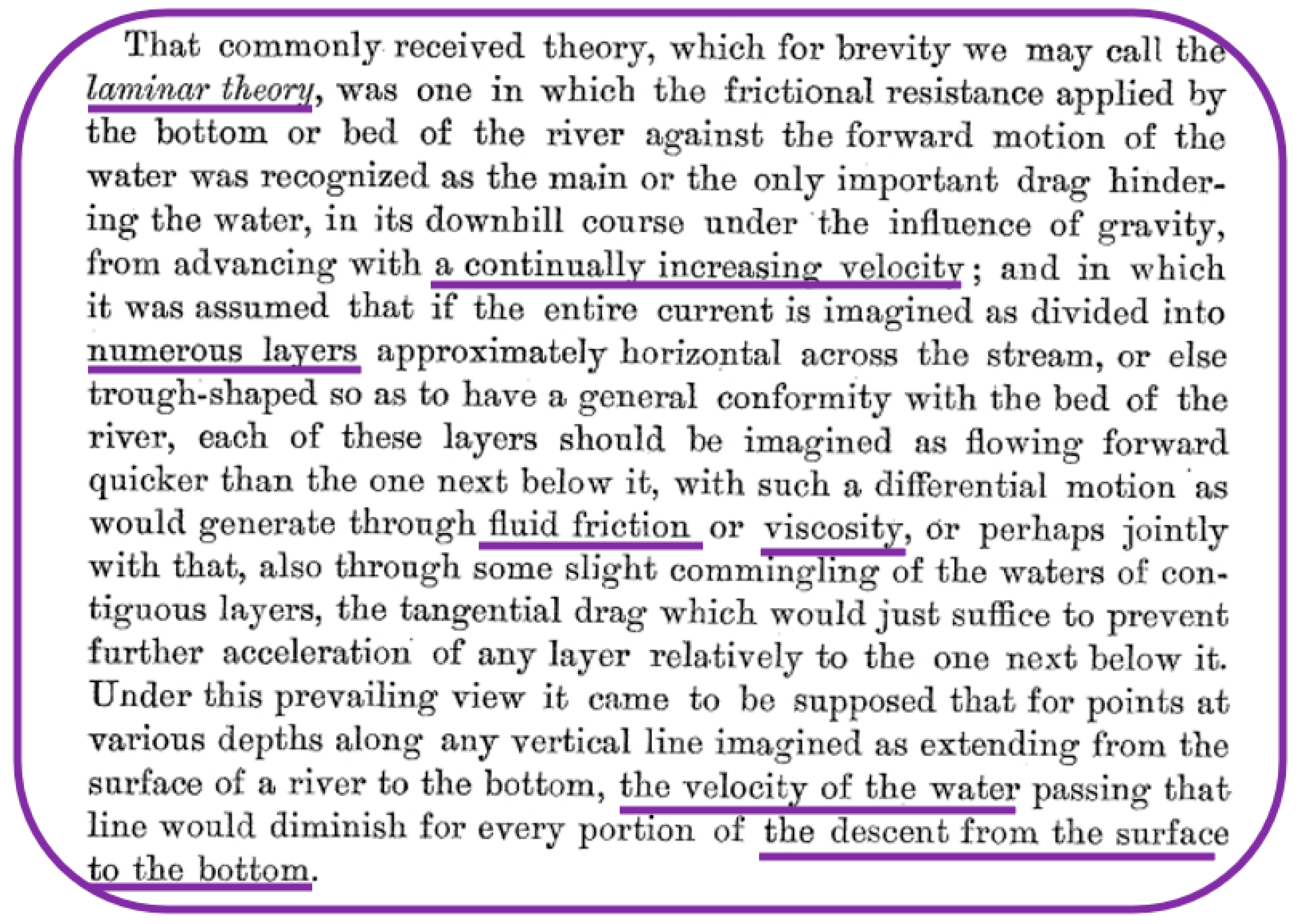
3. James Thomson’s Laminar Theory of the Flow in Rivers and Other Open Channels

Before we proceed to Kelvin’s elementary studies of turbulence, laminar and turbulent motion, and homogeneous, isotropic turbulence, it would be interesting to know whether or not he derived any inspiration from others. James Thomson (1822–1892) was a Professor of Civil Engineering and Mechanics at the University of Glasgow [54] (J.T.B. 1893). He was the two years older brother of William Thomson (Thomson [55] 1887e, page 348, paragraph 2, lines 7–8).
As shown in Figure 3, the definition, causes, and characteristics of the laminar theory are given in (James) Thomson [56] (1878, page 114, paragraph 2, lines 2–5). Key words in Figure 3 are underlined in Purple. Laminar theory is characterized by ‘a continually increasing velocity’ and ‘numerous layers’. It is caused by ‘fluid friction’ or ‘viscosity’, or ‘perhaps jointly with that’, and ‘tangential drag’. It is noted that the ‘velocity of the water’ should decrease ‘from the surface to the bottom’ because of the effect of bottom friction.
(James) Thomson’s [56] (1878) quote of “some slight comingling of the waters of contiguous layers” is the exact notion of gradient transport hypothesis or eddy viscosity evident in many works, which could have its connection with Saint-Venant’s and Boussinesq’s remarkable work as presented in Section 2.
From a historical perspective, the significance of (James) Thomson’s [56] (1878) ‘laminar theory’ is twofold. On the one hand, it might have stimulated the development of Thomson’s [57] (1887d) notions of ‘laminar motion’ and ‘turbulent motion’. On the other hand, it seems to give an early elementary concept of the laminar boundary layer, which was mathematically described by Prandtl [58] (1905).

4. Kelvin’s Elementary Studies of Homogeneous, Isotropic Turbulence

William Thomson, 1st Baron Kelvin (later Lord Kelvin) (26 June 1824–17 December 1907) was a Scots Irish mathematical physicist and engineer (left in Figure 4). Before he entered the University of Cambridge, Thomson was already intrigued with Fourier’s [59] (1822) Theorie Analytique de la Chaleur.
From a historical perspective, in 1887, Kelvin published a series of five papers on the stability of fluid motion [55,57,60,61,62] (Thomson 1887a, b, c, d, and e). Kelvin’s studies of turbulence are conceptual, physical, and mathematical [55,57] (Thomson 1887d, e). Their significance has been gradually realized (e.g., Frisch [1] 1995, page 9, paragraph 1, lines 1–2; Ecke [63] 2005, page 128, 1st paragraph/right column; Frisch et al. [64] 2005, page 1, lines 1–3/right column; Craik [65] 2012, page 94; Schmitt [66] 2017; Shi [50] 2021b, page 4, Section B.; page 7, Section G.). It seems that Thomson [57] (1887e) takes the early elementary investigation of turbulent motion into a special subject and reveals the language and the concepts that future turbulence research must use. However, after having looked a little deeper into what the two papers contained, in particular, Thomson [57] (1887e), a more detailed account of Kelvin’s contributions to turbulence is still required. In fact, some new findings can be highlighted.

4.1. The Early Ideas of Turbulence and Laminar and Turbulent Motion

In his studies of river flow, Thomson [55] (1887d, page 272, paragraph 1, line 18; page 278, line 7) seems to first coin the English word ‘turbulence’ in the scientific literature. This is highlighted in Schmitt [66] (2017). In the meantime, however, ‘the laminar motion (or flow)’ and ‘the turbulent (or tumultuous) motion’, as two important ideas, also seem to first appear eight times in Thomson [55] (1887d, page 272, paragraph 1, lines 11 and 18; page 275, (b), line 2; page 276, 48., lines 18 and 22; page 277, 50., lines 2 and 9; page 278, line 5). This simple but important note seems to be neglected in the literature.

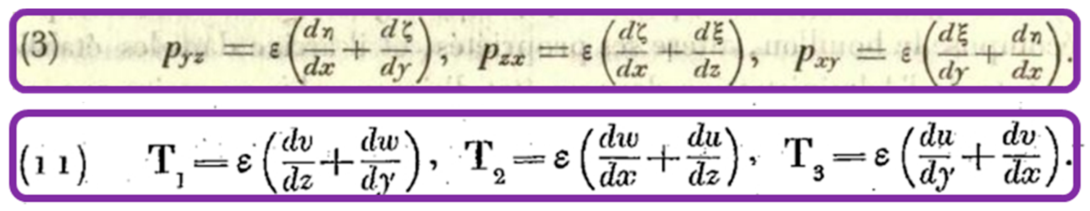
4.2. The ‘Reynolds Stresses’ Anticipated by Kelvin

In his paper On the Dynamical Theory of Gases, Maxwell [67] (1867, page 70, Equations (60)–(62)) develops the following mathematical expressions for the quantities of momentum transferred across the plane in the positive direction ( x ) and the directions of y and z across the same plane, respectively:
u u u ρ + ξ 2 ¯ ρ
u u v ρ + ξ η ¯ ρ
u u w ρ + ξ ζ ¯ ρ
where (2) is the whole momentum in the direction of x of the molecules projected from the negative to the positive side of the plane in units of time. (3) and (4) refer to a transference of momentum in the directions of y and z across the same plane. ξ 2 ¯ , ξ η ¯ , and ξ ζ ¯ represent the mean values of these products.
According to Maxwell [67] (1867, page 70, paragraph 4), if the plane moves with the mean velocity u of the fluid, the total force exerted on the medium on the positive side by the projection of molecules into it from the negative side will be as follows:
A normal pressure ξ 2 ¯ ρ in the direction of x ;
A tangential pressure ξ η ¯ ρ in the direction of y ;
A tangential pressure ξ ζ ¯ ρ in the direction of z .
According to Thomson [57] (1887e, page 345, 7., paragraph 2), the general expression for nullity of translational movement in large volumes may be written as follows:
0 = ave   u = ave   v = ave   w
where ‘ ave ’ denotes the average via any great length of a straight or curved line, or area of the plane or curved surface, or via any great volume of space.
Then, in terms of this generalized notation of averages, homogeneousness implies (Thomson [57] (1887e, 8., Equations (21) and (22)):
ave   u 2 = U 2 ,       ave   v 2 = V 2 ,       ave   w 2 = W 2
ave   v w = A 2 ,       ave   w u = B 2 ,         ave   u v = C 2
where U , V , W , A , B , and C are six velocities independent of the positions of the spaces in which the averages are taken. However, Equations (6) and (7) are infinitely short of implying, although implied, by homogeneousness.
Thomson himself does not realize the significance of the above equations. He emphasizes that ‘These equations are, however, infinitely short of implying, although implied by, homogeneous’. However, actually, he anticipates ‘Reynolds stresses’. If we make a comparison between Maxwell [67] (1867, page 70, Equations (60)–(62)) and Thomson [57] (1887e, page 345, 8., Equations (21) and (22)), it can be found that the terms, ξ 2 ¯ , ξ η ¯ and ξ ζ ¯ , are analogous to those in Equations (4) and (5). This is pointed out by Craik [65] (2012, page 94, paragraph 2 and footnote 15). However, a more detailed account of this point is given in this review. Other implications of Thomson [57] (1887e, page 345, 8., Equation (22)) will be discussed later.

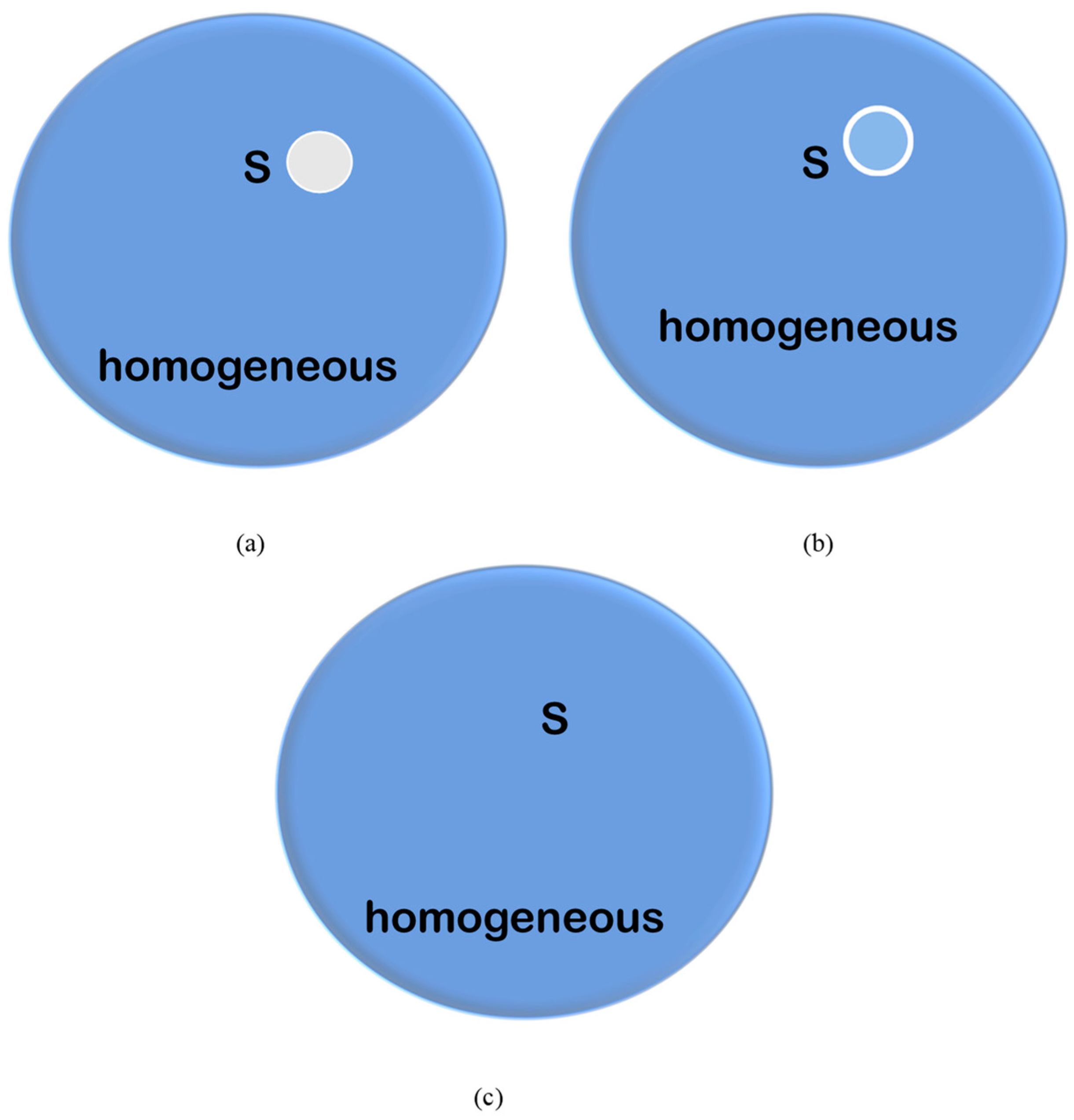
4.3. The Early Concepts of Homogeneous Isotropic Turbulence, Homogeneousness, and Isotropy

‘If an incompressible fluid which is homogeneous or…’ appears in Stokes [68] (1843, page 51, footnote*, line 1). ‘a homogeneous incompressible fluid’ appears in Stokes [69] (1845, page 310, paragraph 3, line 3). It can be believed that the word ‘homogeneous’ in ‘homogeneous isotropic turbulence’ may originate from the early mathematical studies of fluid motion, e.g., Stokes [68,69] (1843, 1845).
However, if we take another look at Thomson’s [57] (1887e) On the propagation of laminar motion through a turbulently moving inviscid liquid, we will be able to see that Thomson [57] (1887e) should be credited for the early concepts of homogeneous, isotropic turbulence and isotropy. Below are the details of the appearances of those notions in Thomson [57] (1887e):
  • homogeneously’ appears four times in Thomson [57] (1887e, page 345, 7. line 1, 8. lines 1, 2, and 8);
  • homogeneous’ eight times in Thomson [57] (1887e, page 346, lines 3, 4, 6, 7, 9, 11, 15; page 352, 24. line 13);
  • homogeneousness’ three times in Thomson [57] (1887e, page 350, line 7; page 352, 24. line 12; page 352, 24. line 12);
  • isotropic’ four times in Thomson [57] (1887e, page 345, 9. line 1; page 346, 13. line 3; page 348, line 19, 17. line 4);
  • isotropy’ seven times in Thomson [57] (1887e, page 348, lines 1–2; page 349, 18. line 9, 19. 8; page 350, 20. lines 8, 14, 16 and 18);
  • homogeneous and isotropic’ two times in Thomson [57] (1887e, page 346, 14. lines 1–2; page 347, 15. lines 2–3).
They are also given mathematical definitions (Thomson [57] 1887e, page 345, Equations (21)–(24)). In particular, Thomson [57] (1887e, page 345, 9.) supposes the distribution of motion to be isotropic and introduces a notion, R , to denote ‘THE AVERAGE VELOCITY of the turbulent motion’:
U 2 = V 2 = W 2 = 1 3 R 2

4.4. The Introduction of Fourier Principles into the Turbulent Flow

By the use of Fourier–Sturm–Liouville analysis, Thomson [55] (1887d, page 273, Equation (63)) gives the following expression:
v = e i ω t + m x + q z 𝒱
Unsurprisingly, in the analysis of turbulent motion, Thomson [57] (1887e, page 343, Section 3) uses Fourier’s principles. Thomson [57] (1887e, page 343, Section 3) formally introduces Fourier principles into the studies of turbulence literature. On Fourier’s principles, we have, as a perfectly comprehensive expression for the motion at any point (Thomson [57] (1887e, page 343, 3., Equations (6)–(9))),
u =   α m , n , q e , f , g sin ( m x + e ) cos n y + f cos ( q z + g )
v =   β m , n , q e , f , g cos ( m x + e ) sin n y + f cos ( q z + g )
w =   γ m , n , q e , f , g cos ( m x + e ) cos n y + f sin ( q z + g )
where α m , n , q e , f , g , β m , n , q e , f , g , γ m , n , q e , f , g are any three velocities satisfying the equation
0 = m α m , n , q e , f , g + n β m , n , q e , f , g + q γ m , n , q e , f , g
and summation (or integration) for different values of m ,   n ,   q ,   e ,   f ,   and   g .

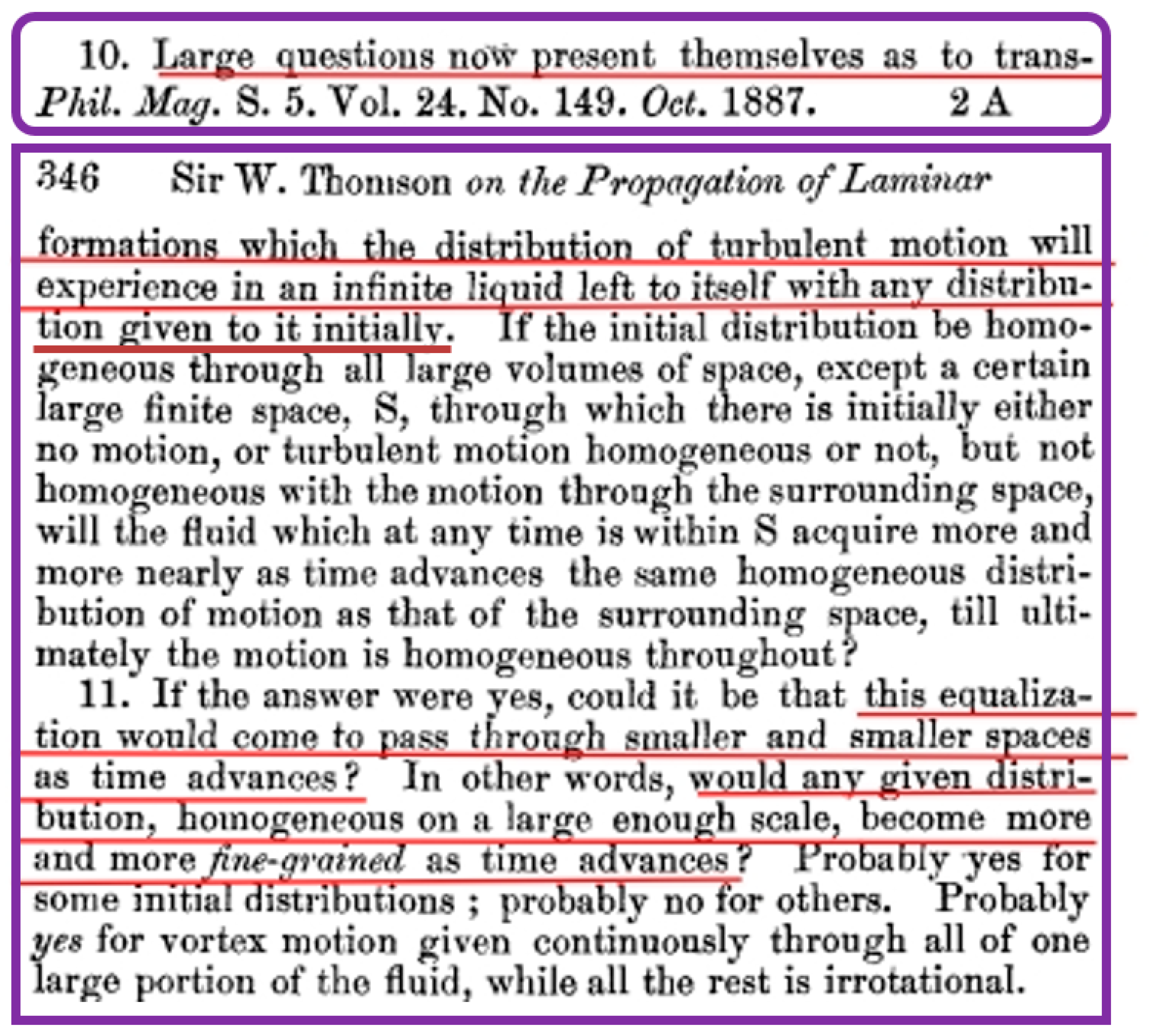
4.5. Transformations Which the Distribution of Turbulent Motion Will Experience

As shown in Figure 5, in Thomson [57] (1887e, page 345, 10.), firstly, Kelvin specifies ‘Large questions’ at the beginning. What does ‘Large’ really mean? In the present author’s view, it may mean: (i) ‘physically important’, which may be a key physical process/mechanism; (ii) ‘hard’, which implies interesting but complex; and (iii) ‘uncertain’, which requires further investigation. Secondly, Kelvin specifies ‘transformations’. Clearly, it should refer to ‘turbulence energy transformations’.
Based on Thomson [57] (1887e, pages 345–346, 10), as interpreted/shown in Figure 6, there are three possible non-uniform homogeneous cases for the initial condition: (a) no motion in space S, but homogeneous in the surrounding space; (b) turbulent motion homogeneous in space S, but not the same homogeneous with the surrounding space; (c) turbulent but not homogeneous motion in space S, but homogeneous in the surrounding space.

4.6. The Kelvin Elementary Concept of the Direct Energy Cascade

These lines underlined in red at the bottom of the bottom panel in Figure 7 can be rewritten as (Thomson [57] 1887e, page 346, 11):
‘…this equalization would come to pass through smaller and smaller spaces as time advances?… would any given distribution, homogeneous on a large enough scale, become more and more fine-grained as time advances?’
As shown in Figure 7, the present author interprets with caution ‘distribution of turbulent motion’ as turbulent eddy, ‘smaller and smaller space’ as the size of the turbulence eddy, and ‘fine-grained’ as the smaller turbulent eddy as well. It is clear that Kelvin has a physical picture of the ‘energy cascade’ even if he is not so sure about it. However, he did not explain what causes the energy cascade; in other words, he did NOT YET attribute ‘viscosity’ to the energy cascade. In the present author’s view, even if Kelvin’s thought is premature, he at least anticipates the elementary concept of direct energy cascade.

4.7. The Concept of the Symmetrical Motion of Vortex Rings

The notion of ‘Motion symmetrical about an ax is’ appears in Stokes [70] (1842). The notion of ‘a stable symmetrical distribution of vortex rings’ appears in Thomson [57] (1887e, page 351, 22., lines 1–2) while ‘the symmetrical arrangement is stable’ in Thomson [57] (1887e, page 351, 23., last line) and ‘symmetrical arrangement’ in Thomson [57] (1887e, page 351, 24., line 4). Furthermore, ‘the steady symmetrical motion’ appears in Thomson [57] (1887e, page 352, 24., lines 8–9) while ‘the symmetrical motion is unstable’ in Thomson [57] (1887e, page 352, 24., line 10). Although those are presented and discussed with reference to the distribution of vortex rings, in the present author’s view, they can be cautiously regarded as the early studies of symmetrical motion in homogeneous, isotropic turbulence. Kelvin’s ‘symmetrical motion’ may have stimulated symmetrical consideration in turbulence. For example, Frisch [71] (1985, page 76, 2.) highlights ‘intermittency as a broken symmetry’. ‘Symmetry consideration is indeed central to the study of both transition phenomena and fully developed turbulence’ (Frisch [1] 1995, page 2).

5. The Maxwell–Reynolds Decomposition of Turbulent Flow Velocity

The conceptual or pictorial decomposition of turbulent wake flow can return to Leonardo da Vinci’s (ca. 1510) drawing Sketch of turbulent wakes of cylinders. For details, see Piomelli [72] (2014). From a historical perspective, this generally anticipates Reynolds’ [73] (1895) decomposition. However, as a simple question, did the idea of the decomposition of turbulent flow velocity directly come into Reynolds’ mind? Is there any early study before Reynolds [73] (1895) which might have inspired his thinking? In his paper On The Dynamical Theory of Gases, Maxwell [67] (1867, page 68) presents the mathematical/physical decomposition of the mean velocity of all the molecules that are at a given instant in a given element of volume and the relative velocity of one of these molecules with respect to the mean velocity, i.e.,
u + ξ ,   v + η ,   w + ζ
where u , v , and w are the components of the mean velocity of all the molecules and ξ , η , and ζ are the components of the relative velocity of one of these molecules with respect to the mean velocity.
Reynolds [73] (1895) is generally viewed as the real start of theoretical studies of turbulence. Reynolds [73] (1895, page 125, paragraph 2 from bottom; page 128, paragraph 3) gives the following notions:
  • Mean-mean-motion: mean-molar u ¯   v ¯   w ¯ ;
  • Relative-mean-motion: relative-molar u   v   w .
Reynolds [73] (1895, page 140, relation (11)) presents the following mathematical equations showing the decomposition of turbulent flow velocity:
u = u ¯ + u ,   v = v ¯ + v ,   w = w ¯ + w
If we make a comparison between Maxwell’s [67] (1867) decomposition and Reynolds’ [73] (1895) decomposition, it can be easily found that they are mathematically/physically the same. In the present author’s view, as a revisionist aspect, it should be called the Maxwell–Reynolds decomposition of turbulent flow velocity. The decomposition or the separation of the velocity u can enable us to isolate the velocity component u x ,   t which is independent of the mean flow. This decomposition or the separation is significant in the definition of locally isotropic turbulence (see Monin and Yaglom [43] 1975, Section 21.2).

6. The Taylor Statistical Theory of Isotropic Turbulence: A Revisit

Geoffrey Ingram Taylor (1886–1975) (right in Figure 4) was a great mathematical physicist. Generally speaking, the early concept of ‘homogeneous, isotropic turbulence’ has been attributed to G.I. Taylor.
Taylor’s contributions to turbulence are best presented in Batchelor [74,75] (1976, 1996) and Sreenivasan [76] (2011). The present review can only be a small supplement to them. Two notes are made: (i) to be consistent with BIBLIOGRAPHY in Batchelor [74] (1976, pages 623–633), the letter after the publication year is adopted here; (ii) to highlight the possible historical significance in this review, however, the first ‘year’ refers to ‘Received or Read year’ while the second ‘year’ to ‘Publication year’.
What motivated Taylor to study turbulence? How did he gradually move on to the statistical studies of turbulence? Is there any connection between Thomson [56,57] (1887d, e) and Taylor’s work on turbulence? To understand the historical development of Taylor’s statistical theory of homogeneous, isotropic turbulence, it is helpful to take an overview of his early work related to the mathematical and physical aspects of turbulence as much as we can.

6.1. The Taylor Concepts of the Average Height and a Coefficient of Eddy Viscosity

In much the same way as for a solid possessing a large coefficient of conductivity, the equation for the propagation of heat by means of eddies in the air is written as (Taylor [7] 1914/1915, page 4, Equation (1)):
θ t = w ¯ d 2 2 θ z 2
where θ is the potential temperature; w ¯ the average vertical velocity of the air in places where it is moving upwards; d  the average height through which an eddy moves from the layer at which it was at the same temperature as its surroundings to the layer with which it mixes. This may be taken to be roughly equal to the diameter of a circular eddy (Taylor [77] 1918, page 137, bottom line).
Taylor [7] (1915, page 14, line 3) writes the following equation:
μ ρ = w ¯ d 2
where μ is the eddy (dynamical) viscosity; ρ the density of the air; w ¯ the average vertical velocity of the air; and d the average height through which an eddy moves from the layer at which it was at the same temperature as its surroundings to the layer with which it mixes.
Two interesting, important concepts in Taylor [7] (1914/1915) have been gradually discovered by the turbulence community:
(i) ‘the average height’: it is indeed physically analogously to Prandtl’s [53] (1925) concept of ‘the mixing length’. This seems to be found by Taylor [78] (1970, page 7, paragraph 4), although it was also pointed out in Frisch [1] (1995, page 222, bottom). Interestingly, however, there was a difference between Prandtl’s [53] (1925) conception and Taylor’s [7] (1914/1915). For details, please refer to Taylor [78] (1970, pages 7–8)
(ii) ‘a coefficient of eddy viscosity’: Taylor [7] (1915, page 13, paragraph 5, lines 7–8) defines ‘a coefficient of eddy viscosity’ equal to ρ × average value of w z z 0 .   w z z 0 is expressed in the form 1 2 w ¯ d , which is actually the turbulent eddy viscosity ( v t ).
This suggests that Taylor [7] (1915) made his attempt at the early mathematical modeling of turbulent motion via the turbulent eddy viscosity ( ρ w ¯ d 2 ), as already pointed out by Hanjalic and Launder [79] (2020, page 297, paragraph 2).
The term w ¯ d 2 appears 14 times in Taylor [7] (1915). Furthermore, K may roughly be taken as equal to 1 2 w d , and it has been discussed in detail in Taylor [77] (1918). K , which is the “eddy conductivity” (Taylor [7] 1915, page 4, paragraph 3, lines 6–7), is proportional to the velocity and to the scale of the turbulence (Taylor [77] 1918, page 137, paragraph 4, line 3). Clearly, we can infer that ‘the scale of the turbulence’ should refer to 1 2 d . This might be the early concept of the Taylor length scale of turbulence. ‘The divisor 2 is inserted because the air at any given point is equally likely to be in any portion of the path of an eddy so that the average value of z z 0 should be approximately equal to 1 2 d ’ (Taylor [7] 1915, page 4, paragraph 1).

6.2. The Taylor Concept of the “Age” of the Eddy

In his study of On the dissipation of eddies, Taylor [80] (1919, page 75, Equation (7)) derives the following:
R = 2 v t
where t evidently represents the time taken by the eddy to attain a radius R starting from the condition in which the dynamic viscosity v is infinite at time t   = 0. Taylor [80] (1919, page 75, line 13) suggests that ‘We may call this the “age” of the eddy.’ Equation (17) can be rewritten as follows:
t = R 2 2 v
This is the mathematical expression of the age of the eddy. That is to say, the age of the eddy ( t ) is a function of a radius ( R ) and the dynamic viscosity ( v ). In the present author’s view, it can be simply called ‘the Taylor age of the eddy’, which should be significant in our understanding of the physics of turbulence, including homogeneous, isotropic turbulence.

6.3. The Early Taylor Concept of the Integral Scale

To have a complete theoretical analogy between molecular and turbulent transfer, Taylor [7] (1914/1915) thought up some length connected with turbulence, which is analogous to the mean length of the paths of molecules.
However, the early concept of the ‘integral scale’ is developed in finding the average value of u(xa) over a large area of a plane perpendicular to the axis of x and integrating via time t (Taylor [13] 1921, page 197, line 9 from the bottom):
x a = 0 t u d t

6.4. How Was the Concept of the Correlation Coefficient Introduced into Turbulence?

According to Taylor [78] (1970, page 8, paragraph 4, lines 5–6), understanding the diffusion of a smoke plume led him to think of ways other than mixture theory to describe turbulent diffusion. In his own words, in the study as presented in Taylor [13] (1921), the idea of correlation was for the first time introduced into the subject.

6.5. The Application of the Discontinuous Motion

Where did Taylor derive the physical inspiration from? As presented in Taylor [81] (1910), it is from Stokes’s [82] (1848) On a Difficulty in the Theory of Sound, which begins with a physical interpretation of Poisson’s integral equation of the motion of a gas in one dimension.

6.6. Taylor’s Own Experimental Studies of the Isotropy of Turbulence

Taylor [7] (1914/1915, page 1, paragraph 3, lines 2–4) writes that the vertical component of wind velocity is very small compared with the horizontal velocity.
However, on 16 March 1927, G.I. Taylor delivered The G.J. Symons Memorial Lecture before the Royal Meteorological Society; in his published lecture entitled Turbulence, Taylor [8] (1927e, page 210, lines 2–5) writes that the average value of the component of eddy velocity in a vertical direction is equal to the average horizontal component in a direction at right angles to the mean wind.
This is shown in Taylor [8] (1927e, Face page 205/Figure 8) based on a record taken at a height of 25 ft. above grassland. Taylor did not interpret this phenomenon as the isotropy of turbulence until Taylor [14] (1935c, page 430, bottom; page 431, top). On a historical note, the isotropy of turbulence is also experimentally verified by Taylor’s graduate student, Donald Campbell MacPhail (1915–1999); for the details, see MacPhail [83] (1940).

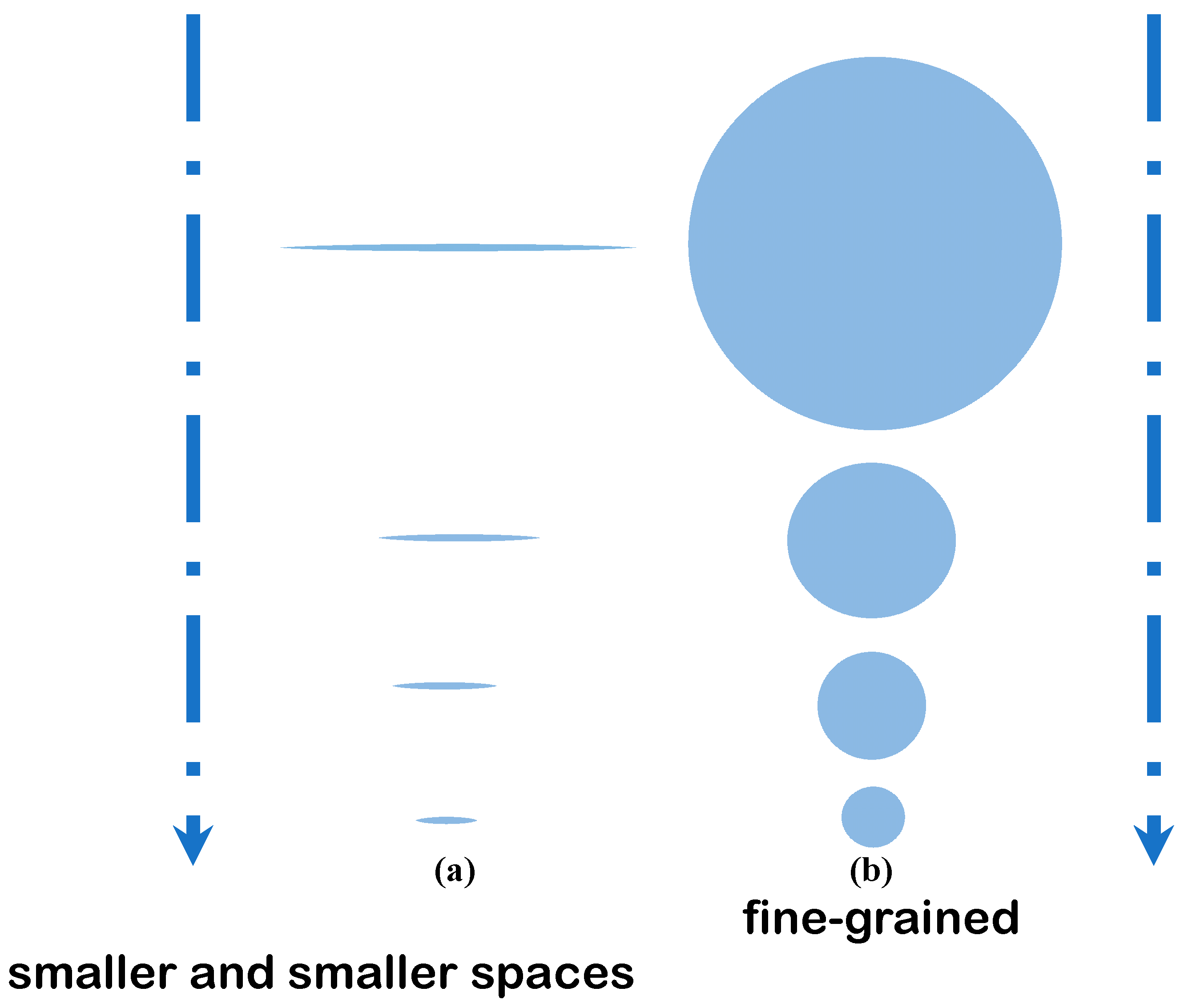
6.7. The Concept of Small Eddies or Microturbulence or Small-Scale Turbulence

The concept of small eddies or microturbulence or small-scale turbulence has been very useful and important throughout the studies of isotropic turbulence. Who introduced the original concept of small eddies or microturbulence or small-scale turbulence?
In his own words (Batchelor’s [84] (1975)), Taylor replied to Batchelor: “I did realize as far as back as 1917 that there must be something that gives small-scale turbulence a statistically isotropic character and this would be a result of some universal quality in the grinding-down process.”
The notion of ‘small eddies’ does appear in Taylor’s [80] (1918/1919, page 73, line 1; page 74, lines 1 and 9) ON THE DISSIPATION OF EDDIES. Taylor [80] (1918/1919) further specifies that…eddy here considered is the type which will arise from the dissipation of an eddy which was originally concentrated in a very small region near the axis.
Taylor [80] (1918/1919) also discusses whether viscosity alone was responsible for the dissipation of the eddies. However, the notion of ‘turbulence’ never appears in Taylor [80] (1918/1919).
The notion of ‘microturbulence’ can be found in Fage and Townend [11] (1932, page 656, line 6). It refers to turbulence, ‘especially near the boundary of the fluid where the scale of the turbulence is small’ (Fage and Townend [11] 1932, page 656, lines 6–7). The notion of ‘small-scale turbulence’ appears in Townend [12] (1934, page 188, paragraph 1, line 10). Simply because of Fage and Townend’s communication with Taylor, this notion does inspire Taylor’s thinking. The notions ‘microturbulence’ and ‘small-scale eddies’, which are highlighted in italics by the present author, appear in Taylor [14] (1935c, page 430, paragraph 2, lines 1–3):
Besides the motions that are chiefly responsible for the diffusive power of turbulence, the whole field may be in a state of microturbulence, i.e., there may exist very small-scale eddies which, although they play a very small part in diffusion, yet may be the principal agents in the dissipation of energy. They may also be the principal causes of the effects of turbulence on the boundary layer in wind tunnels because the absolute magnitude of the space rates of change in pressure may depend on them.
The notion of ‘microturbulence’ also appears in Taylor [14] (1935c, page 437, line 4). The ‘microturbulence’ of Fage and Townend [11] (1932, page 656, line 6) refers to the small scale of the turbulence, but the ‘microturbulence’ or ‘small-scale eddies’ of Taylor [14] (1935c, page 430, paragraph 2, lines 1–3) to the physical significance of the small scale of the turbulence, i.e., the dissipation of energy. The concept of microturbulence is twofold: on the one hand, it is geometrically small; on the other hand, it is physically the principal agent in the dissipation of energy and the principal cause of the effects of turbulence on the boundary layer.
Taylor [14] (1935c, page 437, Second Section) presents in detail the statistical representation of microturbulence. The following length scale, λ , as a measure of the diameters of the smallest eddies which are responsible for the dissipation of energy, is derived (Taylor [14] 1935c, page 437, Equation (48)):
1 λ 2 = Lt y 0 1 R y y 2
where R y is the coefficient of correlation; y is the coordinate in the horizontal direction; and Lt is the Limit.
In the present author’s view, the extensive ‘small-scale turbulence’ studies’ were likely stimulated by the early studies in Taylor’ [80] (1918/1919), Fage and Townend [11] (1934, page 656, lines 6–7) and Taylor [14] (1935c, page 430, paragraph 2, lines 1–3; page 437, line 4). Based on the above presentation, the present author suggests the notion of ‘the Taylor–Fage–Townend concept of small eddies or microturbulence or small-scale turbulence’. This important point regarding the early or original concept of small-scale turbulence is generally omitted in the review literature, including the present author’s own review article (Shi [50] 2021b).

7. The Kolmogorov–Obukhov Scaling Laws: A Revisit

The basis of Kolmogorov’s [28,29] (1941a, c) two hypotheses was the notion of kinetic energy ‘cascading’ from components of the fluctuating turbulent motion with large length scales to components with smaller length scales as a consequence of nonlinear inertial interaction of different components, a notion which was familiar from previous work of G.I. Taylor and L.F. Richardson in particular (Batchelor [85] 1990, page 47, paragraph 2/lines 1–5). Apparently, the basis of Kolmogorov’s [28,29] (1941a, c) two hypotheses was also familiar from Thomson [55] (1887e, page 346, Section 11) as shown in Figure 4 and Figure 6. However, details of the derivation of the Kolmogorov–Obukhov scaling laws and their different physical/mathematical approaches are not really available in the existing literature. The present author feels that there is still a need to revisit the Kolmogorov–Obukhov scaling laws.
As to the priority or order of precedence in Kolmogorov’s and Obukhov’s publications, Professor Katepalli R. Sreenivasan shared an interesting anecdote with the present author in an e-mail dated 6 February 2024: “On Kolmogorov and Obukhov, Yaglom told me once that Obukhov gave his draft paper to Kolmogorov who wrote his own paper very quickly after that. Kolmogorov had been examining wind velocity records and thinking of the problem for some time, and his ideas were independent and expressed quite differently, but the timing of the publication was motivated by Obukhov. I cannot directly verify it, of course”.

7.1. The k 5 / 3 Power Law for the Turbulence Energy Spectrum Function E k

To give the readers a clear timeline, the following short review is presented in chronological order. Kolmogorov [28,29] (1941a, page 13, Equation (23); 1941c, page 16, Equation (9)) derived the 2/3 power law for the second-order structure function within the inertial subrange:
B d d r ~ C ϵ ¯ 2 3 r   2 3
The k 5 / 3 power law for the turbulent energy spectrum function E k within the inertial subrange was explicitly included in Obukhov [86,87,88,89] (1941a, page 461, Equation (38); 1941b, page 466, Equation (14); 1941c, page 24, Equation (14); 1941d, page 21, Equation (14)). Note that Obukhov [86] (1941a) refers to a long version in Russian, Obukhov [87] (1941b) to a short version in German, Obukhov [88] (1941c) to a short version in Russian, and Obukhov [89] (1941d) to a short version in English translated by V. Levin. However, one more step is needed before the k 5 / 3 power law for the turbulent energy spectrum function E k can be fully obtained within the inertial subrange when k is large enough.
The following key derivations are made from the full version in Russian:
Obukhov [86] (1941a, page 457, Equation (16)) defines the following:
E p = M p v 2 2 = p φ k d k
where E p is the energy; φ k is the energy distribution.
Obukhov [86] (1941a, page 457, Equation (19)) forms the balance equation for the turbulent energy:
T p = D p + E p t
where T p is the transformation of energy from the macrofield in the unit of time; D p the dissipation of energy in the velocity field of the microcomponent due to viscosity forces; E p is the energy distribution.
Obukhov [86] (1941a, page 461, Equation (38)) obtains
E p 2 3 κ 2 3 D 0 2 3 p 2 3
where κ is a particular numerical constant; D 0 the initial dissipation of energy; and p the observation frequency.
The k 5 / 3 power law for the turbulence energy spectrum function E k seems to be explicitly included in Obukhov [86] (1941a, page 461, Equation (38)) since it can be obtained via differentiation from the above Equation (24).
To the best knowledge of the present author, the modern form of the k 5 / 3 power law for the turbulence energy spectrum function E k does not appear in the English literature until Batchelor and Townsend [90] (1949, page 240, Equation (2.1)):
E k = A ϵ 2 3 k 5 3
where A is an absolute constant; ϵ the turbulent dissipation rate; and k the wave number.

7.2. Obukhov’s [86] (1941a) Motivation of Studies of the Spectral Balance of Energy

What is Obukhov’s motivation for studies of the spectral balance of energy? There is an interesting footnote* on page 453 in Obukhov [86] (1941a). Professor Sergey Chefranov has kindly translated those lines into English:
The approach to the mathematical processing of the Richardson scheme adopted by use of the following presentation was proposed by A.N. Kolmogorov in a report read at the Institute of Theoretical Geophysics at the end of 1939. In this report, it was indicated that for the middle values of frequencies, the function E p introduced below should have the form E p = C p α . However, A.N. Kolmogorov failed to determine the value of the exponent α in 1939. We shall show that α = 2 3 based on the equation of the spectral balance of energy.
Clearly, in a way, Obukhov [86] (1941a, page 461, Equation (38)) was an extension of Kolmogorov’s unsolved frequency function in 1939.

7.3. The Obukhov Concept of a Function of the Inner Reynolds Number

Notably, there is another interesting footnote* for κ in Obukhov [89] (1941d, page 21):
Generally speaking, κ ought to be a function of the inner Reynolds’ number R e * = E 1 / 2 l ν , but for large R e * it is natural to assume that κ is constant.
Clearly, ‘the inner Reynolds’ number ( R e * ) used by Obukhov refers to the Taylor-microscale Reynolds number ( R e λ ).

7.4. The Relationship between Kolmogorov [28,29] (1941a, c) and Obukhov [86,87,88,89] (1941a, b, c, d)

What exactly is the relationship between Kolmogorov [28,29] (1941a, c) and Obukhov [86,87,88,89] (1941a, b, c, d)? Are they similar or the same work? Do they use a similar approach or the same approach? Did they interact with each other? Kolmogorov [28] (1941a) was received on 28 December 1940, Kolmogorov [29] (1941c) on 30 April 1941, and Obukhov [86] (1941a) on 28 April 1941, Obukhov [88] (1941c) on 4 May 1941. Yaglom [91] (1990, page vi, bottom line; page vii, lines 1–12) gives all the answers, but Kolmogorov himself often emphasized that only the statement of the problem is due to him while the main quantitative results were obtained independently by him and Obukhov during a period when they were separated. Therefore, it is not surprising that the approach used by the two authors was quite different. Kolmogorov’s study was based on general dimensional arguments combined with some physical ideas about the mechanism of developed turbulence, related to ideas stated during the twenties by L.F. Richardson, while Obukhov considered a model semiempirical equation for the spectrum of turbulence (it was the first two-point closure in the mechanics of turbulence) and demonstrated an amazing physical intuition by extracting from this equation only the consequences which are, in fact, universal and do not depend on the particular closure hypothesis used. The formulation of the main result by Kolmogorov and Obukhov was also quite different.
In Obukhov’s obituary, however, Yaglom [91] (1990, page vii, paragraph 1, lines 12–19) gives a nice summary:
Kolmogorov described the small-scale structure of turbulence by the so-called structure function of the velocity field (i.e., by the dependence on r of the mean square of the velocity difference at two points spaced r cm apart) and derived the ‘2/3 power law’ for the structure function, while Obukhov used the power spectrum of the velocity field and obtained the spectral ‘-5/3 power law’. These two laws are mathematically equivalent, but the simplicity of the spectral measurements made the ‘-5/3 power law’ the basic universal law of small-scale turbulence structure.
Yaglom [91] (1990, page vii, paragraph 2, bottom) re-iterates that ‘but in Obukhov [86] (1941a) the spectral representation of the velocity field itself was also considered and used to derive the universal ‘-5/3’ power law.’ For the sake of consistency, ‘1941b’ is replaced by ‘1941a’.
To take another look at those lines above, we can see that Kolmogorov and Obukhov use different approaches and obtain different formulations of their main results, which are mathematically equivalent.
After his reading of Batchelor’s [84] (1975) An unfinished dialogue with G.I. Taylor, Professor Sreenivasan understands that Taylor did not fully appreciate the depth and innovation of Kolmogorov’s far-reaching ideas. Coincidently, Professor Lord Julian C.R. Hunt shared an anecdote with a similar view to the present author, as included in Shi [50] (2021b, page 14).

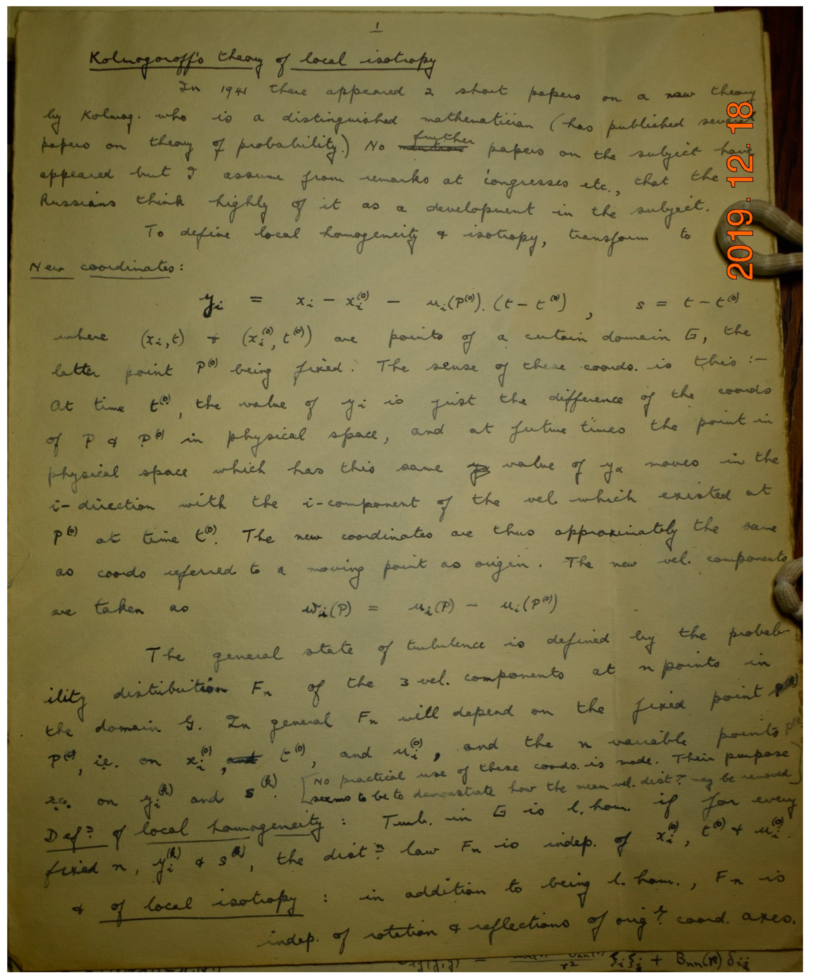
7.5. Batchelor’s Dissemination of Kolmogorov’s Theory of Local Isotropy: A Revisit

How/why did Kolmogoroff’s [Kolmogorov’s] theory of local isotropy attract Batchelor’s attention and interest? As shown in Figure 8, in his own words, Batchelor wrote,
“Kolmogoroff’s theory of local isotropy
In 1941, there appeared 2 short papers on a new theory by Kolmog. [Kolmogoroff or Kolmogorov] who is a distinguished mathematician (has published several papers on theory of probability). No further papers on the subject have appeared but I assume from remarks at congresses etc., that the Russians think highly of it as a development in the subject.”
From the above lines, Kolmogoroff’s [Kolmogorov’s] theory of local isotropy attracted Batchelor’s attention, and interest seems to be from Kolmogorov’s fellow Russians’ remarks at Congresses. Batchelor must have met and talked with those Russians there. This is also reflected in Batchelor [92] (1947, page 533, paragraph 2, lines 5–8).
Only two short papers giving a bare outline of the theory have appeared in a language other than Russian, but from remarks of a general nature made at a scientific meeting in Moscow (4), it seems that the theory is widely known within the U.S.S.R. and is held in high regard.
Obukhov [89] (1941d) was cited in Batchelor [93] (1946b). It is unclear why Batchelor did not see the merit of Obukhov [89] (1941d, page 21, Equation (14)), which can be mathematically equivalent to the k 5 / 3 spectrum and the ‘2/3 power law’ for the structure function in Kolmogorov [28] (1941a, page 13, Equation (23); 1941c, page 16, Equation (9)).
After Taylor’s further studies of “microturbulence” and “small-scale eddies”, Kolmogorov [28,29] (1941a, c) moved on and made his great contribution to it. What was the motivation for small-scale eddies studies at Cambridge, U.K., in the middle of the 1940s when Batchelor and Alan Townsend were there? Townsend [94] (1990, page 2, paragraph 2, lines 3–9) seems to give the answer clearly:
At that time [ca. 1945], I was reliant on George [Batchelor] to suggest the measurements of grid turbulence that could be useful. He [George Batchelor] had found the work of A.N. Kolmogorov on local isotropy of the small-scale eddies, which seemed to open a route to the understanding of inhomogeneous and shear flows. A test of the prediction of form for the structure function in the inertial range could not be made in our small tunnel, and verification (in terms of the spectrum function) had to wait on Bob (R.W.) Stewart’s work in the ocean.

8. The Heisenberg Statistical Theory of Homogeneous, Isotropic Turbulence

What motivated Heisenberg to study the statistical and isotropic turbulence, particularly the spectrum for eddies at low Reynolds numbers? By using a similarity hypothesis, the spectrum for eddies at large Reynolds number was indirectly determined by Kolmogorov [28,29] (1941a, c) and directly by Onsager [95] (1945) and von Weizsaecker [96] (1948). Heisenberg [31] (1948a) has gone further by including those frequency components at low Reynolds numbers. However, based on Liepmann [97] (1952b, page 411, bottom note), Kolmogorov, Onsager, and von Weizsacker did not actually use the spectrum concept. The result for the spectrum is actually due to Heisenberg [31] (1948a).

8.1. Heisenberg’s Inverse Seventh Power Spectrum

The following equation is for the dissipation of energy (Heisenberg [31] 1948a, German version, page 632, Equation (13)):
S k = μ + ρ κ k d k F k k 3 0 k F k 2 k 2 d k
where S k is the total loss of the energy of that part of the spectrum that is contained between k = 0 and k ; k the wave number; μ the viscosity; ρ the density; κ a numerical constant; k ; F k and F k the intensity of the small eddies.
It was rewritten as (Heisenberg [32] 1948b, English version, page 402, Equation (1)):
S k = μ + ρ κ k F k k 3 d k 0 k 2 F k k 2 d k
After the publications of Heisenberg [31] (1948a) in German and Heisenberg [32] (1948b) in English, they were of interest to a number of prominent physicists and applied mathematicians, e.g., Tchen, Corrsin, Chandrasekhar, Lee, Batchelor, Hopf, and Proudman.
As a historical note, in his letter to Batchelor dated 15 March 1953, it can be inferred that Heisenberg wrote his paper (Heisenberg [32] 1948b) in English entitled On the theory of statistical and isotropic turbulence when he was retained in Farmhall at Godmanchester, U.K. Heisenberg [32] (1948b) in English was submitted to Proceedings of the Royal Society of London via G.I. Taylor who visited Heisenberg at Godmanchester, Cambridgeshire, England. As the second historical note, Batchelor sent the proofs to Heisenberg when he was at Godmanchester.

8.2. Chandrasekhar’s Thought on Heisenberg [31,32] (1948a, b)

Chandrasekhar [38] (1949d, page 335, paragraph 3) wrote the following:
While Kolmogoroff’s method of determining the form of the equilibrium spectrum of fully developed turbulence is very elegant, it does not, one must admit, give any real insight into the physical nature of turbulence. Also, even under equilibrium conditions, it does not give the part of the spectrum in which the dissipation by viscosity begins to be an important factor. An elementary theory that clearly visualizes the phenomenon of turbulence, and which gives, at the same time, the complete equilibrium spectrum, is due to Heisenberg [31,32].
Equation (19b) was again rewritten as (Chandrasekhar [35] (1949b, page 336, Equation (18)):
ϵ k = 2 ρ ν + κ k F k k 3 d k 0 k F k k 2 d k
Clearly, Chandrasekhar thought that Heisenberg’s [32] (1948b) theory of turbulence is better than Kolmogorov’s [28,29] (1941a, c), i.e., the former gives both a real insight into the physical nature of turbulence and the complete equilibrium spectrum of turbulence. Were Chandrasekhar’s justifications really right? The interaction between Chandrasekhar and Heisenberg can be found in a recent review (Sreenivasan [98] 2019, page 6, Section 2.1, paragraph 1; page 7/Figure 3).

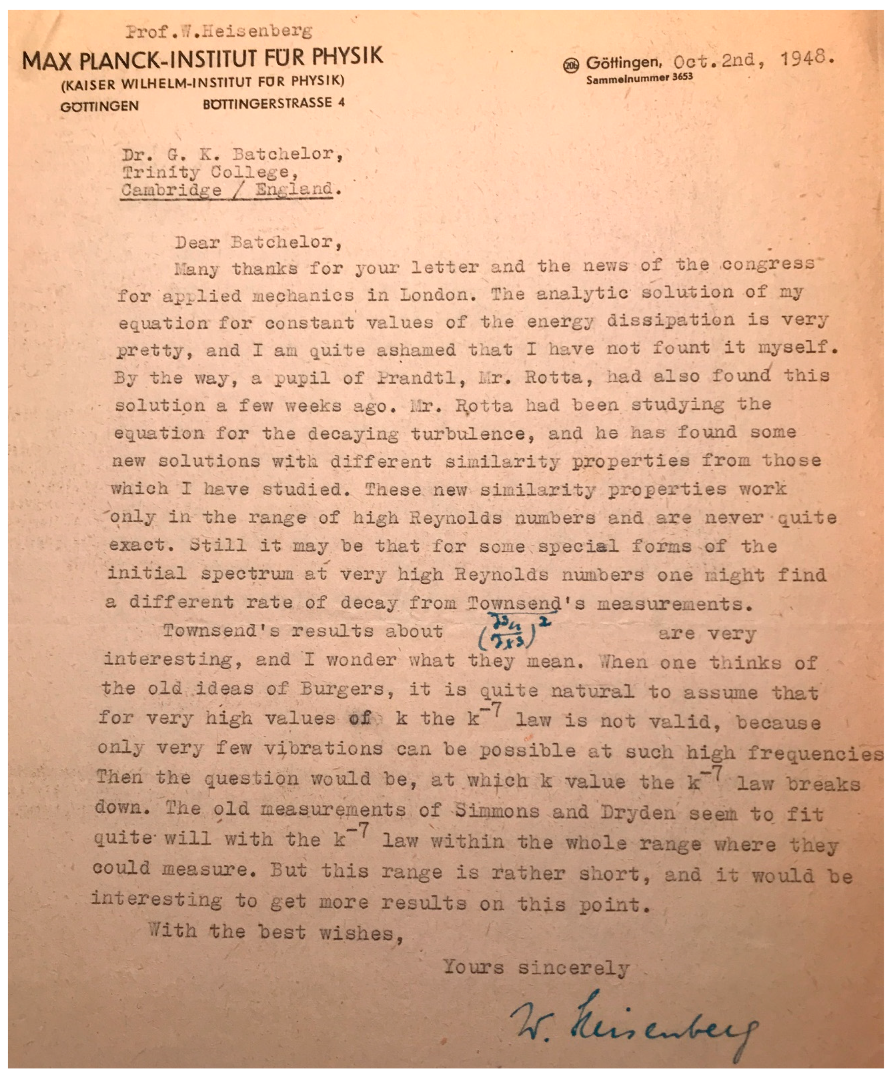
8.3. Heisenberg’s Own Thoughts on His Inverse Seventh Power Spectrum

What are Heisenberg’s own thoughts on his inverse seventh power spectrum? How did he debate with Batchelor? In his letter to Batchelor dated 2 October 1948, as shown in Figure 9, Heisenberg wrote that the following:
 
Dr. G.K. Batchelor,
Trinity College,
Cambridge/England
 
Dear Batchelor,
 
Many thanks for your letter and the news of the congress for applied mechanics in London. The analytic solution of my equation for constant values of the energy dissipation is very pretty, and I am ashamed that I have not fount [found] it myself. By the way, a pupil of Prandtl, Mr. Rotta, had also found this solution a few weeks ago. Mr. Rotta had been studying the equation for the decaying turbulence, and he has found some new solutions with different similarity properties from those which I have studied. These new similarity properties work only in the range of high Reynolds numbers and are never quite exact. Still it may be that for some special forms of the initial spectrum at very high Reynolds numbers one might find a different rate of decay from Townsend’s measurements.
Townsends’s results about 3 u x 3 2 ¯ are very interesting, and I wonder what they mean. When one thinks of the old ideas of Burgers, it is quite natural to assume that for very high values of k the k 7 law is not valid, because only very few vibrations can be possible at such high frequency. Then the question would be, at which k value the k 7 law breaks down. The old measurements of Simmons and Dryden seem to fit will [well] with the k 7 law within the whole range where they could measure. But this range is rather short, and it would be interesting to get more results on this point.
 
With the best wishes,
 
Yours sincerely
Figure 9. A photograph of Heisenberg’s letter to Batchelor dated 2 October 1948. Courtesy of the Wren Library, Trinity College, Cambridge, U.K. and reproduced with permission.
Atmosphere 15 00494 g009

8.4. Batchelor’s Thoughts on Heisenberg [31,32] (1948a, b)

What were Batchelor’s thoughts on Heisenberg’s [31,32] (1948a, b) theory? Provided that the measure quantities can be interpreted in the manner assumed by the equilibrium theory, the high measured value of D 6 D 4 2 D 2 must be regarded as evidence in favor of Heisenberg’s expression of the spectrum and of the existence of an upper limit to the extent of the spectrum (Batchelor and Townsend [90] 1949, page 252). An overview of Heisenberg’s form of the energy spectrum in the quasi-equilibrium range can be found in Batchelor [40] (1953, pages 161–168, Section 7.5).

8.5. Corrsin’s Indirect Thought on Heisenberg [31,32] (1948a, b)

In Corrsin’s letter to Batchelor dated February 18, 1947, Corrsin wrote the following:
“On the matter of isotropic turbulence, one of our graduate students is working earnestly on reconciling the Kolmogoroff-Obukoff [Obukhov] and Weissacker-Heisenberg analyses. Heisenberg’s analysis in the range of viscous dissipation seems unjustifiable, from simple dimensional reasoning”.

8.6. C-M Tchen’s Thoughts on Heisenberg [31,32] (1948a, b)

By using the harmonic analysis of the Navier–Stokes equation, Tchen [99] (1954) investigated the transfer of energy across the spectrum. Furthermore, he tried to determine the phase correlation entering into the transfer by the statistical considerations of transport processes. The results allow a theoretical explanation with regard to the Heisenberg and Obukhov postulates, delimiting the conditions of their applicability. The Heisenberg theory of turbulence was based on turbulent dissipation, while the Obukhov theory of turbulence is based on turbulent shear (Tchen [99] 1954, page 4). According to Tchen [96] (1954, page 4), Obukhov’s [86] (1941a) theory of turbulence is different from Heisenberg’s [31,32] (1948a, b).

8.7. Monin and Yaglom’s Thought on Heisenberg [31,32] (1948a, b)

Heisenberg [31] (1948a) has extended those calculations by Kolmogoroff [28,29] (1941a, c), Onsager [95] (1945), and von Weizsaecker [96] (1948) to include those frequency components which have small Reynolds numbers. Does it really mean that the Heisenberg hypothesis and its inverse seventh power law are valid for small Reynolds numbers only?
Monin and Yaglom [43] (1975, page 229/Equation (17.40)) obtain the following energy spectrum corresponding to the Heisenberg hypothesis as k :
E k = 4 3 4 3 γ H 2 / 3 ε 2 / 3 k 5 / 3 1 + 8 3 γ H 2 k k η 4 4 / 3
where γ H is a dimensionless constant. The above equation seems to be suitable for all k . This was already pointed out by other people, e.g., Chandrasekhar [36] (1949c) and Monin and Yaglom [53] (1975, page 229). It is shown that the asymptotic relationships, E k ~ k 5 / 3 and E k ~ k 7 , can be obtained from Equation (22) (Monin and Yaglom [53] 1975, page 229).

8.8. Townsend’s Thought on Heisenberg [31,32] (1948a, b)

Townsend [94] (1990, page 2, paragraph 5, lines 1–7; page 3, paragraph 1, line 1) wrote that the following:
I started a series of spectrum measurements of grid turbulence to test the validity of the Heisenberg inverse seventh power spectrum for the far viscous range. In a moment of inspiration, I decided that the power could be obtained by measuring the flatness factors of a number of high-order velocity derivatives, and I managed it for the first four. The kurtosis increased both with order of the derivative and with the Reynolds number of the turbulence. I then realised that the measurements said nothing about the spectrum, but they did show a considerable departure from the predictions of local similarity.

9. Discussion

‘Science cannot solve the ultimate mystery of Nature. And that is because, in the last analysis, we ourselves are part of the mystery that we are trying to solve.’
Max Planck (1858–1947)

9.1. Does (James) Thomson’s [56] (1878) Laminar Theory Inspire William Thomson [57] (1887d)?

In the present author’s view, the answer should be yes. In some way, the general rise of these concepts in research on turbulence is shown in (James) Thomson [56] (1878) and Thomson [55,57,60,61] (1887a, b, c, d, e). The original notion used by Kelvin is turbulent motion, which appears nine times in Thomson [57] (1887e, page 342, line 1; page 346, lines 1 and 6; page 348, lines 22, 23 and 26, and 33; page 349, line 10; page 351, line 1). ‘turbulence’ was mentioned in Davidson, Kaneda, Moffatt, and Sreenivasan [100] (2011, page 427, line 16).

9.2. Does Kelvin Anticipate the Correlation Coefficient of the Velocities at Two Different Points?

Are there any other implications in Thomson [57] (1887e)? Firstly, following up Taylor [13] (1921, page 205, paragraph 3, line 3; page 207, Equation (18)), the fundamental correlation coefficient  R i j of the velocities at two different points, is given in Robertson [27] (1940, page 210, Equation (1.2)):
u 2 ¯ R i j u i u j ¯
If we compare Thomson [57] (1887e, page 345, 8., Equation (22)) and Robertson [27] (1940, page 210, Equation (1.2)), it can be seen that R i j is also hidden in Thomson [57] (1887e, page 345, 8., Equation (22)) and its value is 1.
Secondly, suppose the distribution of turbulent motion to be isotropic, Thomson [57] (1887e, page 345, Equation (24)) obtains
0 = A = B = C
This actually implies that there is no correlation between any two ( v w ,   w u ,   u v ) in Thomson [57] (1887e, page 345, Equation (22)). Thomson did not realize this. However, this became an important argument in Taylor [13] (1921, page 199, paragraph 4, lines 3–4) for this application of the coefficient of correlation or correlation coefficient R ξ . In a way, Thomson [57] (1887e, page 345, 8., Equations (22) and (24)) anticipates the early concept of the correlation coefficient R i j or R ξ .

9.3. The Relationship between Kelvin’s and G.I. Taylor’s Studies of Isotropic Turbulence

How would Kelvin’s early studies of homogeneous, isotropic turbulence have mathematically and physically inspired those studies by others, e.g., G.I. Taylor? Although Kelvin’s studies of homogeneous, isotropic turbulence were not cited in Taylor’s studies of turbulence, it still can be believed that the former has furthered the latter since those concepts of Kelvin are used or further developed by Taylor.
Is there any link between Kelvin’s isotropic turbulence and Taylor’s assumption of isotropy? The notion of isotropy was introduced by Taylor in 1935 (Batchelor [101] 1946a, page 480, 1st paragraph). It is still true. However, from a historical perspective, it is evident that Thomson’s early elementary concept of isotropy should have stimulated the further development of Taylor’s notion of isotropy even though Taylor had not referred to Thomson in his papers. Based on this selective review, they seem to be independent. Thomson [57] (1887e, page 345, Equation (23)) is the early elementary concept of isotropy, which was further developed in Taylor [14] (1935c, page 431, Equation (20)):
u x 2 ¯ = v y 2 ¯ = w z 2 ¯ u y 2 ¯ = u z 2 ¯ = v x 2 ¯ = v z 2 ¯ = w x 2 ¯ = w y 2 ¯ v x u y ¯ = w y v z ¯ = u z w x ¯
After the assumption of (statistical) isotropy, however, the fractions, 1 8 , 1 8 , 1 9 , 2 9 , 2 9 , 1 9 , appear in Thomson [57] (1887e, page 350, Equations (46)–(51)) while the integers, instead, 3 and 6, in Taylor [14] (1935c, page 433, Table I).

9.4. Implication of Kelvin’s Elementary Fourier Analysis of Turbulent Motion

Does Thomson’s [55,57] (1887d, e) elementary Fourier analysis of turbulent motion anticipate the theory of turbulence by Orszag and Kruskal [102] (1968) and Orszag [103] (1970) and stimulate the development of Direct Numerical Simulation of three-dimensional homogeneous isotropic turbulence by Orszag [103] (1970) and Orszag and Patterson [104] (1972)? In the present author’s view, from a historical perspective, the idea of Direct Numerical Simulation of isotropic turbulence is rooted in Kelvin’s early elementary Fourier analysis of turbulence motion.

9.5. Does Kelvin Anticipate the Concept of the Energy Cascade?

According to Batchelor’s [84] (1975) ‘An unfinished dialogue with G.I. Taylor’, Taylor had ideas about the energy cascade in 1917, but he did not see how to express them in mathematical form. The present author believes it is true. In his definition of ‘small eddies’, Taylor [80] (1918/1919) also emphasizes that the following:
All eddies will, in fact, tend to this type [small eddies] by the time their radii have increased till they are large compared with their original radii.
The notions of ‘large eddies’ and ‘small eddies’ can be found in Taylor [80] (1919). ‘All eddies will in fact tend to this type’ may imply the idea about the energy cascade. Taylor also highlights that the motion will be determined by viscosity in the case of small or slowly rotating eddies only.
Nevertheless, the energy cascade in turbulence has generally been thought to be expressed in the following poem (Richardson [105] 1922, page 66, paragraph 3, bottom):
“big whirls have little whirls that feed on their velocity, and little whirls have lesser whirls and so on to viscosity—in the molecular sense”.
Based on this selective review above, the present author feels that the elementary concept of the energy cascade is hidden in Thomson [57] (1887e, page 346, Section 11) and Figure 6, even though he did not attribute ‘viscosity’ to the energy cascade. Taylor’s idea about the energy cascade is not very clear. The Kelvin–Richardson–Onsager energy cascade is suggested; for details, see Shi [50] (2021b).

9.6. Does the Taylor Age of ‘Eddy’ Anticipate the Kolmogorov Time Scale?

The Kolmogorov time scale is expressed as Kolmogorov [28] (1941a):
σ = 1 a = v ε ¯
It is unclear whether there is any relationship between the Taylor age of the eddy (Taylor [80] 1918/1919) and the Kolmogorov time scale (Kolmogorov [28] 1941a, page 302, Equation (18), in Russian). In the present author’s view, there should be some relationship between them even though they are not the same. A simple question can be raised: does the Taylor age of ‘eddy’ anticipate the Kolmogorov time scale?

9.7. What Was the Genesis of the Concept/Theory of Isotropic Turbulence?

What was the genesis of the concept/theory of isotropic turbulence? After taking a look at Taylor’s [78] (1970, page 8, paragraph 5, lines 1–12) remarks, Sreenivasan [76] (2011, page 144, paragraph 2, line 1) writes that ‘This was the genesis of isotropic turbulence…’.
Based on this selective review, from a historical perspective, three general stages can be roughly identified:
(i) Kelvin’s elementary statistical and physical studies of homogeneous, isotropic turbulence in the 1880s.
(ii) Experimental investigations or statistical measurements of (isotropic) turbulence in the 1920s and 1930s. For example, in particular, Dryden [24] (1939, page 417, paragraph 3) highlights the existence of isotropic turbulence for the following two cases:
one in which the changes in magnitude and in direction are wholly random and the fluctuations are statistically the same at every point of the field; the turbulence at the center of a pipe in which the flow is eddying or in the natural wind at a sufficient height above the ground is approximately isotropic.
(iii) The gradual development of Taylor’s statistical theory of isotropic turbulence in the 1920s and 1930s.

9.8. Does Obukhov Anticipate the Finite Reynolds Number Effect of Turbulence?

Does Obukhov’s footnote* [89] (1941d, page 21, footnote*) have any significant implications for the studies of isotropic turbulence or small-scale turbulence? The present author cautiously thinks that C in Kolmogorov [28,29] (1941a, page 13, Equation (23); 1941c, page 16, Equations (9) and (19)) is analogous to κ in Obukhov [89] (1941d, page 21, footnote*), i.e., C . also ought to be a function of the Taylor-microscale Reynolds number ( R e λ ), but for large R e λ it is natural to assume that C is (Kolmogorov) constant.
This early but important point is consistent with those studies made in the late 1990s, e.g., Gamard and George [106] (1999, page 443, Abstract, line 9) in which C in a power law is Reynolds number dependent, while in the limit of infinite Reynolds number, C is a constant. This also has implications for the studies of the finite Reynolds number effect of turbulence [107] (Qian 1997) and the Reynolds number dependence of energy spectra in the overlap region of isotropic turbulence (Gamard and George [106] 1999). In the present author’s view, Obukhov’s footnote* [89] (1941d, page 21, footnote*) anticipates the finite Reynolds number effect of turbulence, or the finite Reynolds number effect of turbulence is hidden in Obukhov’s footnote* [89] (1941d, page 21, footnote*).
According to Djenidi and Antonia [108] (2020), Obukhov [109] (1962) was also thinking about a Finite Reynolds Number effect (rather than an intermittency effect, as allegedly proposed by his master).

9.9. Some Remarks on the Different Derivations of the k 5 / 3 Power Law

In the present author’s view, some remarks are still required to be made regarding the different derivations of the k 5 / 3 power law. These should include the following:
(i) For smaller k (i.e., for large Reynolds numbers of the eddies), the following mathematical expression for the intensity F k of the small eddies is found in von Weizsacker [96] (1946/1948, page 624, Equation (32)): F k   ~   k 5 / 3 . For smaller k (i.e., for large Reynolds numbers of the eddies), the following mathematical expression for the intensity F k of the small eddies is found in Heisenberg [31] (1946/1948a, page 629, paragraph 2, lines 13 and 15; page 630, line 5 from the bottom; page 631, line 8 from the bottom; page 652, line 5; 1948b, page 403, paragraph 2, line 3): F k   ~   k 5 / 3 . In addition, the k 5 / 3 term appears a number of times in Heisenberg [31] (1946/1948a). The “ k 5 / 3 ” and its power law for the turbulent energy spectrum function within the inertial range first explicitly appears in Batchelor [93] (1946b, page 884, left column, lines 17–18): ‘the energy per unit wave-number ( k ) is proportional to k 5 / 3 ’.
(ii) Batchelor and Townsend [90] (1949, page 240) call Equation (19) ‘the form of the equilibrium spectrum’. There are several interesting points: (a) Why is not Equation (19), i.e., the form of the equilibrium spectrum, derived in Batchelor [93] (1946b) and Batchelor’s masterly interpretation of the Kolmogorov theory of turbulence (Batchelor [92] 1947)? (b) Batchelor and Townsend [90] (1949) consider the implications of Kolmogorov’s theory for the spectrum function E k ; however, they seem to derive Equation (19) from their Equation (1.8), i.e., they had their own derivation, and Equation (19) was NOT derived from Equation (18) (Obukhov [86] 1941a, page 461, Equation (38). (c) Is A really an absolute constant?
(iii) It is generally well known that the same k 5 / 3 power law of energy spectrum within the inertial range alone can be obtained by dimensional arguments despite different physical foundations of theories of turbulence or different approaches, but not in other ranges. Why? An explanation is given in Tchen [99] (1954). The metamorphosis of turbulence suggests that there are phenomena (or stages): production, transfer, and dissipation. In Tchen’s view, as long as the dimensional reasonings appropriately present the transfer in a simple way, any dimensionally correct expression of transfer will be expected to lead to the same k 5 / 3 power law.
(iv) Kolmogorov–Obukhov’s k 5 / 3 power law seems to simply be derived by the appropriate use of dimensional analysis regardless of both the viscous effect and the large-scale effect. Does it imply that the infinite Reynolds number limit is insignificant in this respect? Obviously, the answer is no. The Reynolds number has to be infinite. In general, the spectrum E k , say, will depend on ϵ , k , and ν . In the first (K41) hypothesis, all three parameters are retained, thus leading to E * k = f u n c t i o n   k * , where the asterisk ( ) denotes normalization by the Kolmogorov scales. In the inertial range, ν is eliminated so that E k now depends only on ϵ and k (second K41 hypothesis, at least in the spectral domain). The dimensional analysis then leads to the following: E k is proportional to k 5 3 .
(v) There are possible shortcomings of dimensional analysis, even though Kolmogorov’s [28,29] (1941a, c) derivation, which was (more or less) emulated by Batchelor [92] (1947), seems reasonably convincing, especially since the Kármán–Howarth equation admits a similarity solution based on the Kolmogorov parameters. This is strictly true if you have incomplete similarity (i.e., the effect of the large-scale term in the KH equation is neglected). For complete similarity, i.e., similarity at all scales, Kolmogorov scaling is possible only when R λ remains constant throughout the decay, e.g., Dryden [37] (1943), Batchelor [40] (1953), Hinze [5] (1958), and Djenidi and Antonia [110] (2015).
(vi) Onsager’s derivation of -5/3 power law first appears in his own one-page Abstract Onsager [92] (1945), introduced in Batchelor [93] (1946b), and re-derived in Onsager [111] (1949). Based on David McComb’s e-mail to the present author, the proper derivation is carried out in wavenumber space (Onsager) and does not rely on the vague concept of the cascade. Instead, it arises from the scale invariance of the energy flux, and this is precisely defined. Generations of theoretical physicists have been happy with this and do not have the conceptual problems of those who work in real space. Strictly speaking, from an ontological point of view, one should derive the k 5 / 3 spectrum from Onsager’s approach and then obtain the r 2 / 3 structure function by Fourier transform.
If we take another look at them, however, Onsager’s [111] (1949) work (9 pages) is NOT a full version of Onsager’s [92] (1945) Abstract (1 page) at all. Clearly, the approach shown in Onsager [95] (1945) is NOT used in Onsager [110] (1949) anymore. Instead, Onsager [111] (1949, pages 283–285, Equations (13)–(19)) seems to show the details about how the Navier–Stokes equations (Equation (13)) can lead to the -5/3 power law (Equation (19)) via the Fourier transformation (Equation (19)). Onsager [111] (1949, page 284, bottom paragraph) still discusses an ‘accelerated cascade process’.
From dimensional considerations, Onsager [111] (1949, page 285, Equation (19)) derived the following k 5 / 3 spectrum:
Ω k = β Q 2 / 3 k 5 / 3
where Ω k is the distribution of energy in isotropic turbulence, β a dimensional universal constant, and Q the dissipation.
Onsager [111] (1949, page 286, Equation (24)) derived the following r 2 / 3 structure function by the theory of Fourier transform:
v 2 ¯ R r = v 2 ¯ ( β / 3 Γ 2 / 3 Q r 2 / 3
where v the velocity and R r the correlation function.
(vii) One may be entitled to dismiss the derivation of 2/3 (or -5/3) based on dimensional arguments. But is it a coincidence that there have been other derivations (not based on dimensional arguments)?, e.g., Lundgren’s [112] (2002) derivation based on asymptotic expansions and also that of Djenidi et al. [113] (2019), who examined the consequences of applying scale invariance to the Navier–Stokes equations. Djenidi et al. [114] (2023) and Tang et al. [114] (2023) show that there is a mathematical constraint (essentially arising from the Cauchy-Schwarz inequality) that leads to 2/3. This constraint is related to the Dual Scaling (DS) of the structure function or spectrum. The DS approach in Tang et al. [115] (2023) essentially (with some differences) corresponds, in physical space, to the approach used by Gamard and George [106] (1995) in the spectrum domain. Tang et al. extend the approach to nth-order structure functions.

9.10. Is Heisenberg’s Inverse Seventh Power Spectrum Significant or Insignificant?

Based on the brief review in Section 8, Heisenberg’s inverse seventh power spectrum has been controversial. The present author generally agrees with Chandrasekhar that Heisenberg presents an elementary turbulence theory that visualizes clearly the phenomenon of turbulence and gives the complete equilibrium spectrum. The spectrum was highlighted in Monin and Yaglom [53] (1975, page 229).
The preset author cannot claim to understand Heisenberg’s thoughts and arguments very well. However, based on Heisenberg’s published papers and his unpublished correspondence with others, including the above one with Batchelor, he seems to be always satisfied with his k 7 law.
Heisenberg [32] (1948b, page 406) discusses the effect of viscosity on turbulence. He found that there are two contrasting ideas: (i) turbulence is caused by viscosity, which is true but the old idea; (ii) it is almost the other way round, which is true since turbulence is caused by the energy exerted. An interesting question can be raised: is viscosity important in the generation of turbulence?
According to Sreenivasan, Chandrasekhar was at one time excited by Heisenberg’s theory (when he analytically solved the Heisenberg equation) but was later disappointed when it became known that the inverse seventh power was not supported by experiments. Any such power law is also not shown in the results of Direct Numerical Simulation (e.g., Buaria and Sreenivasan [116] 2020). Professor Katepalli Sreeinvasan also kindly shared the following interesting historical anecdote with the present author in an e-mail dated 22 February 2024:
On 19 June 1950, Chandra wrote to Eberhard Hopf (who had earlier raised specific questions on Heisenberg’s theory) as follows: “And for Heisenberg’s elementary theory: more refined experiments do not support it any way!” Thus, it was clear that by that time, Chandra was disenchanted with Heisenberg’s theory.
As a final note, this review is mainly concerned with inviscid small-scale isotropic turbulence. This aspect of turbulence can be appreciated when the small scale of viscous motion is considered. However, results of DNS by Elsinga et al. [117] (2023) have shown how viscous anisotropic processes have to be considered.

9.11. Where Do These Modern Approaches Currently Stand?

Undoubtedly, after those early studies of isotropic turbulence, both laboratory experiments and direct numerical simulations have made significant progress. As presented in previous sections, there are already a few scattered references to them as being at the leading edge these days in isotropic turbulence research. Where do these modern approaches currently stand in terms of Reynolds number, resolution, etc.? In their direct numerical simulations, Panickacheril et al.’s study [51] (2022, page 6/Table 1) used R λ ,   0 and R λ ,   0 as the initial Reynolds numbers based on the Taylor microscale and integral scale, respectively. For the first case, R λ ,   0 ranges from 9 up to 422, while R L ,   0 ranges from 7 up to 1171. For the second case, R λ ,   0 ranges from 13 up to 456, while R L ,   0 ranges from 9 up to 1476. In terms of resolution, the linear grid size N ranges from 256 to 1024 for the two cases. In their direct numerical simulations up to R e λ = 1445, Elsinga et al. [117] (2023) show that the scaling exponents for the enstrophy and the dissipation rate extrema are different and depend on the Reynolds number.
One may argue that various anecdotes and speculations about who was the first to conceive of some idea and how the generation of past researchers may have influenced each other appear to have occupied a large fraction of space in this article. Perhaps more important is, what theories of the past have significantly impacted the field? What are important questions that have been answered, or are so difficult that they have still not been answered in the year 2024? After all, “who was the first” would not matter so much now, in retrospect, if a theory has been proven to be so insightful. In the present author’s view, one of the major purposes of this article is to present the revisionist aspects since a number of “who was the first” types of questions have not been completely answered before. Consequently, it is true that the style of writing this article is a mix of formal and informal discussion. Since this article is devoted to a historical review of some early scientific works on the study of classic vortical turbulence, those various ‘historical’ anecdotes should be of interest to scientists and engineers in the field of turbulence.

10. Summary

To some extent, this article has focused on purported interactions among historical figures in the field of isotropic turbulence, whose contributions in the years up to the 1950s have been of great impact, i.e., Lord Kelvin vs. Taylor, Kolmogorov vs. Obukhov, Heisenberg vs. Batchelor, etc. The following preliminary findings can be summarized:
(1)
The present author strongly believes that there are still many hidden pearls of mathematical and physical aspects of turbulence in Kelvin’s elementary studies of isotropic turbulence. They were/or will be inspirational to our studies of isotropic turbulence.
(2)
There is about a five-decade span between Kelvin’s early studies of isotropic turbulence and Taylor’s statistical theory of isotropic turbulence. It is still unclear how they are linked. Nevertheless, there must be some connections between them.
(3)
The whole but brief historical narrative may be interpreted as follows: Firstly, the birth of the concept of isotropy in turbulent flow is credited to Kelvin. Secondly, from a historical perspective, Kelvin provided a mathematical and physical study of isotropic turbulence first. Thirdly, Taylor himself first made his observational or experimental investigations of the vertical component and the horizontal component of eddy motion in the atmosphere and did statistical analysis of those results. Fourthly, the early experimental discoveries of isotropy seem to be made by Fage and Townend. The statistical theory of isotropy was further developed by Taylor.
(4)
Kelvin’s introduction of the Fourier Principle into turbulent flow may have anticipated/stimulated the development of Direct Numerical Simulation.
(5)
Coincidently, 26 June 2024 will mark the bicentenary of the birth of Kelvin, while May 7, 2024, the 110th anniversary of Taylor’s first paper on the turbulence of Eddy Motion in the Atmosphere since he read it on 7 May 1914. The present review can be a tribute to Kelvin and G.I. Taylor.
(6)
The Obukhov concept of a function of the inner Reynolds number (i.e., the Reynolds dependent coefficient) anticipates the Finite Reynolds number effect of the turbulence.
(7)
The Kolmogorov–Obukhov scaling laws are indeed significant, but the significance of Heisenberg’s inverse seventh power law should not be underestimated.
(8)
It is hoped that the revisionist aspects, and especially the role of Kelvin presented in this review, are of interest and perhaps inspirational to those studying aspects of isotropic turbulence.
(9)
It is also hoped that this review can be one on establishment and attempts to complete the isotropic turbulence theory.

Funding

This research received no external funding.

Institutional Review Board Statement

Not applicable.

Informed Consent Statement

Not applicable.

Data Availability Statement

Not applicable.

Acknowledgments

David McComb is thanked for inviting the present author to write this review. Stuart B. Dalziel, Director of the G.K. Batchelor Laboratory, is thanked for his arrangement of the present author’s use of the mixing box shown in Figure 1 in the Michaelmas Term of 2019. Meng-Nan Sun is thanked for his discussion about Lord Kelvin’s idea of an energy cascade in 2018. Keith Moffatt is thanked for his encouragement. The Wren Library, Trinity College Cambridge, is thanked for allowing the present author to access the Batchelor Archive. Robert A. Antonia is thanked for his discussion with the present author regarding Kolmogorov—Obukhov’s k 5 / 3 power law as presented in Section 9.9. Sergey Chefranov is thanked for his clarification of Obukhov’s derivation of the energy spectrum. Alain Pumir has kindly helped the present author to understand Saint-Venant [2] (1843). The following people have carefully read and commented on the various versions of this review: David McComb, Lord Julian C.R. Hunt, Katepalli Sreenivasan, Robert A. Antonia, and Sergey Chefranov. Les J. Hamilton kindly made corrections to the three early versions. Katepalli Sreenivasan suggests a few small changes to the 3rd draft that reflect facts better. Antonia and Sreenivasan are thanked for their additional comments received just after the original submission of this manuscript. Four reviewers are thanked for their constructive comments, which have improved the quality of this manuscript. Antonia spotted an error in this final revision. Les J. Hamilton kindly corrected this final revision. The Assistant Editor is thanked for her hard editorial work. The Atmosphere Editorial Office is thanked for their generosity.

Conflicts of Interest

The author declares no conflict of interest.

References

  1. Frisch, U. Turbulence. The Legacy of A.N. Kolmogorov; Cambridge University Press: Cambridge, UK, 1995; p. xiii+296. [Google Scholar]
  2. Saint-Venant, A.J.C. (Barre) de. Note a joindre au Memoire sur la dynamique des fluids. Comptes Rendus Des Seances De L’Academie Des Sci. 1843, XVII, 1240–1243. [Google Scholar]
  3. Helmholtz, L.F. On discontinuous movements of fluids. Philos. Mag. 1868, 36, 337–346. [Google Scholar] [CrossRef]
  4. Prandtl, L. Beitrag Zum Turbulenz Symposium. In Proceedings of the Fifth International Congress of Applied Mechanics, Cambridge, MA, USA, 12–16 September 1938; John Wiley: New York, NY, USA, 1938; pp. 340–346. (In German). [Google Scholar]
  5. Hinze, J.O. Turbulence an Introduction to Its Mechanisms and Theory; McGraw-Hill Book Company, Inc.: New York, NY, USA, 1959; p. ix+586. [Google Scholar]
  6. Gence, J.N. Homogeneous turbulence. Annu. Rev. Fluid Mech. 1983, 15, 201–222. [Google Scholar] [CrossRef]
  7. Taylor, G.I. Eddy motion in the atmosphere. Philos. Trans. R. Soc. Lond. 1915, A215, 1–26. [Google Scholar] [CrossRef]
  8. Taylor, G.I. Turbulence. Q. J. R. Meteorol. Soc. 1927, 53, 201–212. [Google Scholar] [CrossRef]
  9. Dryden, H.L.; Kuethe, A.M. The Measurements of Fluctuations of Air Speed by the Hot-Wire Anemometer; National Advisory Committee for Aeronautics Report No. 320; Bureau of Standards: Washington, DC, USA, 1929; pp. 357–382. [Google Scholar]
  10. Mock, W.C.; Dryden, H.L. Improved Apparatus for the Measurement of Fluctuations of Air Speed in Turbulent Flow; National Advisory Committee for Aeronautics Report No. 448; Bureau of Standards: Washington, DC, USA, 1932; pp. 131–154. [Google Scholar]
  11. Fage, A.; Townend, H.C.H. An examination of turbulent flow with an ultramicroscope. Proc. R. Soc. Lond. 1932, A135, 656–677. [Google Scholar]
  12. Townend, H.C.H. Statistical measurements of turbulence in the flow of air through a pipe. Proc. R. Soc. Lond. 1934, A145, 180–211. [Google Scholar]
  13. Taylor, G.I. Diffusion by continuous movements. Proc. Lond. Math. Soc. 1921, 2, 196–212. [Google Scholar] [CrossRef]
  14. Taylor, G.I. Statistical theory of turbulence. I. Proc. R. Soc. Lond. 1935, A151, 421–444. [Google Scholar] [CrossRef]
  15. Taylor, G.I. Statistical theory of turbulence. II. Proc. R. Soc. Lond. 1935, A151, 444–454. [Google Scholar] [CrossRef]
  16. Taylor, G.I. Statistical theory of turbulence. III. Proc. R. Soc. Lond. 1935, A151, 455–464. [Google Scholar]
  17. Taylor, G.I. Statistical theory of turbulence. IV. Proc. R. Soc. Lond. 1935, A151, 465–478. [Google Scholar]
  18. Taylor, G.I. Statistical theory of turbulence. V. Proc. R. Soc. Lond. 1936, A156, 307–317. [Google Scholar]
  19. Taylor, G.I. The statistical theory of isotropic turbulence. J. Aeronaut. Sci. 1937, 4, 311–317. [Google Scholar] [CrossRef]
  20. Simmons, L.F.G.; Salter, C. Experimental investigation and analysis of the velocity variations in turbulent flow. Proc. R. Soc. Lond. 1934, A145, 212–234. [Google Scholar]
  21. Dryden, H.L. The theory of isotropic turbulence. J. Aeronaut. Sci. 1937, 4, 273–280. [Google Scholar] [CrossRef]
  22. Dryden, H.L.; Schubauer, G.B.; Mock, W.C., Jr.; Skramstad, H.K. Measurements of Intensity and Scale of Wind-Tunnel Turbulence and Their Relation to the Critical Reynolds Number of Spheres; National Advisory Committee for Aeronautics Report No. 581; Bureau of Standards: Washington, DC, USA, 1937; pp. 109–140. [Google Scholar]
  23. Simmons, L.F.G.; Salter, C. An experimental determination of the spectrum of turbulence. Proc. R. Soc. Lond. 1938, A165, 73–89. [Google Scholar]
  24. Dryden, H.L. Turbulence and diffusion. Ind. Eng. Chem. 1939, 31, 416–425. [Google Scholar] [CrossRef]
  25. Von Kármán, T. The fundamentals of the statistical theory of turbulence. J. Aeronaut. Sci. 1937, 4, 131–138. [Google Scholar] [CrossRef]
  26. de Kármán, T.; Howarth, L. On the statistical theory of isotropic turbulence. Proc. R. Soc. Lond. 1938, A164, 192–215. [Google Scholar] [CrossRef]
  27. Robertson, H.P. The invariant theory of isotropic turbulence. Math. Proc. Philos. Soc. 1940, 36, 209–223. [Google Scholar] [CrossRef]
  28. Kolmogorov, A.N. The local structure of turbulence in incompressible viscous fluid for very large Reynolds numbers. Dokl. Akad. Nauk. SSSR 1941, XXX, 299–303. reprinted in Proc. R. Soc. Lond. 1991, A434, 9–13(In Russian) [Google Scholar]
  29. Kolmogorov, A.N. Dissipation of energy in the locally isotropic turbulence. Dokl. Akad. Nauk SSSR 1941, XXXII, 19–21. reprinted in Proc. R. Soc. Lond. 1991, A434, 15–17(In Russian) [Google Scholar]
  30. Millionschikov, M.D. On the uniform isotropic turbulent theory. Dokl. Akad. Nauk. SSSR 1941, XXXII, 611–614. (In Russian) [Google Scholar]
  31. Heisenberg, W. Zur statistischen theorie der turbulenz. Z. Fur Phys. 1948, 124, 628–657. (In German) [Google Scholar] [CrossRef]
  32. Heisenberg, W. On the theory of statistical and isotropic turbulence. Proc. R. Soc. Lond. 1948, A195, 402–406. [Google Scholar]
  33. Lin, C.C. Note on the law of decay of isotropic turbulence. Proc. Natl. Acad. Sci. USA 1948, 34, 540–543. [Google Scholar] [CrossRef] [PubMed]
  34. Chandrasekhar, S. The theory of statistical and isotropic turbulence. Phys. Rev. 1949, 75, 896–897. [Google Scholar] [CrossRef]
  35. Chandrasekhar, S. On the decay of isotropic turbulence. Phys. Rev. 1949, 75, 1454–1455, Erratum in Phys. Rev. 1949, 76, 158. [Google Scholar] [CrossRef]
  36. Chandrasekhar, S. On Heisenberg’s elementary theory of turbulence. Proc. R. Soc. Lond. 1949, 200, 20–33. [Google Scholar]
  37. Dryden, H.L. A review of the statistical theory of turbulence. Q. J. Appl. Math. 1943, 1, 7–42. [Google Scholar] [CrossRef]
  38. Chandrasekhar, S. Turbulence–a physical theory of astrophysical interest. Astrophys. J. 1949, 110, 329–339. [Google Scholar] [CrossRef]
  39. Agostini, L.; Bass, J. The Theories of Turbulence (Translation of Les Theories de la Turbulence. Publications Scientifiques et Techniques du Minjstb de L‘Air, No. 237, 1950); National Advisory Committee For Aeronautics Technical Memorandum No. 1377; Bureau of Standards: Washington, DC, USA, 1950; p. iii+163. [Google Scholar]
  40. Batchelor, G.K. The Theory of Homogeneous Turbulence; Cambridge University Press: Cambridge, UK, 1953; p. xi+197. [Google Scholar]
  41. Leslie, D.C. Developments in the Theory of Turbulence; Oxford University Press: New York, NY, USA, 1973; 368p. [Google Scholar]
  42. Monin, A.S.; Yaglom, A.M. Statistical Fluid Mechanics: Mechanics of Turbulence. Volume I; English ed.; revised by the authors and edited by J.L. Lumley; The Massachusetts Institute of Technology Press: Cambridge, MA, USA, 1971; p. xii+769. [Google Scholar]
  43. Monin, A.S.; Yaglom, A.M. Statistical Fluid Mechanics: Mechanics of Turbulence. Volume II; English ed.; revised by the authors and edited by J.L. Lumley; The Massachusetts Institute of Technology Press: Cambridge, MA, USA, 1975; p. xi+874. [Google Scholar]
  44. McComb, W.D. The Physics of Fluid Turbulence; Clarendon Press: Oxford, UK, 1990; p. xxiv+572. [Google Scholar]
  45. McComb, W.D. Theory of turbulence. Rep. Prog. Phys. 1995, 58, 1117–1206. [Google Scholar] [CrossRef]
  46. Sreenivasan, K.R.; Antonia, R.A. The phenomenology of small-scale turbulence. Annu. Rev. Fluid Mech. 1997, 29, 435–472. [Google Scholar] [CrossRef]
  47. Moffatt, H.K. Homogeneous turbulence: An introductory review. J. Turbul. 2012, 13, N39. [Google Scholar] [CrossRef]
  48. McComb, W.D. Homogeneous, Isotropic Turbulence; Oxford University Press: Oxford, UK, 2014; 429p. [Google Scholar]
  49. Shi, J.Z. George Keith Batchelor’s interaction with Chinese fluid dynamicists and inspirational influence: A historical perspective. Notes Rec. R. Soc. 2021, 75, 461–502. [Google Scholar] [CrossRef]
  50. Shi, J.Z. Qian Jian (1939–2018) and his contribution to small-scale turbulence studies. Phys. Fluids 2021, 33, 041301. [Google Scholar] [CrossRef]
  51. Panickacheril, J.J.; Donzis, D.A.; Sreenivasan, K.R. Laws of turbulence decay from direct numerical simulations. Philos. Trans. R. Soc. Lond. A 2022, A380, 20210089. [Google Scholar] [CrossRef]
  52. Boussinesq, J. Mémoires Présentés par Divers Savants à l‘Académie des Sciences de l‘Institut de France Paris. Essai sur la theorie des eaux courantes. Extr. Des Tomes XXIII Et XXIV 1877, XXII+666. (In French) [Google Scholar]
  53. Prandtl, L. Bericht uber untersuchungen zur ausgebildeten turbulenz. Z. Fur Angew. Math. Und Mech. 1925, 5, 136–139. [Google Scholar] [CrossRef]
  54. J.T.B. Obituary Notices of Fellows Deceased. Proc. R. Soc. Lond. 1893, 52, i–x. [Google Scholar]
  55. Thomson, W. On the propagation of laminar motion through a turbulently moving inviscid liquid. Lond. Edinb. Dublin Philos. Mag. J. Sci. Ser. 1887, 24, 342–353. [Google Scholar] [CrossRef]
  56. Thomson, J. On the flow of water in uniform regime in rivers and other open channels. Proc. R. Soc. Lond. 1878, 28, 113–127. [Google Scholar]
  57. Thomson, W. Stability of motion (continued from the May, June, and August Numbers)—Broad river flowing down an inclined plane bed. Lond. Edinb. Dublin Philos. Mag. J. Sci. 1887, 24, 272–278. [Google Scholar] [CrossRef]
  58. Prandtl, L. Uber Flussigkeitsbewegung bei sehr kleiner Rfibung. In Verhandlungen des Dritten Internationalen Mathematiker-Kongresses; Krazer, A., Ed.; in Heidelberg 1904; Teubner: Leipzig, Germany, 1905; pp. 391–484. (In German) [Google Scholar]
  59. Fourier, J. Theorie Analytique de la Chaleur; A Paris, Chez Firmin Didot, Pere et Fils; Gauthier-Villars: Paris, France, 1822; p. xii+639 pp+2 plates. (In French) [Google Scholar]
  60. Thomson, W. On the stability of steady and of periodic fluid motion. Lond. Edinb. Dublin Philos. Mag. J. Sci. 1887, 23, 459–464. [Google Scholar] [CrossRef]
  61. Thomson, W. On the stability of steady and of periodic fluid motion (continued from May number)—Maximum and minimum energy in vortex motion. Lond. Edinb. Dublin Philos. Mag. J. Sci. 1887, 23, 529–539. [Google Scholar] [CrossRef]
  62. Thomson, W. Stability of fluid motion (continued from the May and June numbers)—Rectilineal motion of viscous fluid between two parallel planes. Lond. Edinb. Dublin Philos. Mag. J. Sci. 1887, 24, 188–196. [Google Scholar] [CrossRef]
  63. Ecke, R. The turbulence problem an experimentalist’s perspective. Los Alamos Sci. 2005, 29, 124–141. [Google Scholar]
  64. Frisch, U.; Bec, J.; Aurell, E. Locally homogeneous turbulence: Is it an inconsistent framework? Phys. Fluids 2005, 17, 081706. [Google Scholar] [CrossRef]
  65. Craik, A.D.D. Lord Kelvin on fluid mechanics. Eur. Phys. J. H 2012, 37, 75–114. [Google Scholar] [CrossRef]
  66. Schmitt, F.G. Turbulence from 1870 to 1920: The birth of a noun and of a concept. Comptes Rendus Mec. 2017, 345, 620–626. [Google Scholar] [CrossRef]
  67. Maxwell, J.C. On the dynamical theory of gases. Philos. Trans. R. Soc. Lond. 1867, 157, 49–88. [Google Scholar]
  68. Stokes, G.G. On some cases of fluid motion. Trans. Camb. Philos. Trans. 1843, VIII, 105–137. [Google Scholar]
  69. Stokes, G.G. On the theories of the internal friction of fluids in motion, and of the equilibrium and motion of elastic solids. Trans. Camb. Philos. Trans. 1845, VIII, 287–319. [Google Scholar]
  70. Stokes, G.G. On the steady motion of incompressible fluids. Trans. Camb. Philos. Trans. 1842, VII, 439–453. [Google Scholar]
  71. Frisch, U. Fully developed turbulence and intermittency. In Turbulence and Predictability in Geophysical Fluid Dynamics and Climate Dynamics; LXXXVIII Corso Soc. Italiana di Fisica: Bologua, Italy, 1985; pp. 71–84. [Google Scholar]
  72. Piomelli, U. Large eddy simulations in 2030 and beyond. Philos. Trans. R. Soc. 2014, A372, 20130320. [Google Scholar] [CrossRef] [PubMed]
  73. Reynolds, O. On the dynamical theory of incompressible viscous fluids and the determination of the criterion. Philos. Trans. R. Soc. Lond. 1895, A186, 123–164. [Google Scholar]
  74. Batchelor, G.K. Geoffrey Ingram Taylor 7 March 1886–27 June 1975. Biogr. Mem. Fellows R. Soc. Lond. 1976, 22, 565–633. [Google Scholar] [CrossRef]
  75. Batchelor, G.K. The Life and Legacy of G.I. Taylor; Cambridge University Press: Cambridge, UK, 1996; p. xv+285. [Google Scholar]
  76. Sreenivasan, K.R. G.I. Taylor: The inspiration behind the Cambridge school. In A Voyage through Turbulence; Davidson, P.A., Kaneda, Y., Moffatt, K., Eds.; Cambridge University Press: Cambridge, UK, 2011; pp. v+127–186. [Google Scholar]
  77. Taylor, G.I. Phenomena connected with turbulence in the lower atmosphere. Proc. R. Soc. Lond. 1918, A94, 113–137. [Google Scholar] [CrossRef]
  78. Taylor, G.I. Some early ideas about turbulence. J. Fluid Mech. 1970, 41, 3–11. [Google Scholar] [CrossRef]
  79. Hanjalic, K.; Launder, B.E. Eddy-viscosity transport modelling: A historical review. In 50 Years of CFD in Engineering Sciences. A Commemorative Volume in Memory of D. Brian Spalding; Runchal, A., Ed.; Springer Nature Singapore Pte Ltd.: Singapore, 2020; pp. 295–316. [Google Scholar]
  80. Taylor, G.I. On the Dissipation of Eddies; Reports and Memoranda No. 598 of Advisory for Committee Aeronautics; Bureau of Standards: Washington, DC, USA, 1919; pp. 73–78. [Google Scholar]
  81. Taylor, G.I. The conditions necessary for discontinuous motion in gases. Proc. R. Soc. Lond. 1910, A84, 371–377. [Google Scholar]
  82. Stokes, G.G. On a difficulty in the theory of sound. Lond. Edinb. Dublin Philos. Mag. J. Sci. 1848, 33, 349–356. [Google Scholar] [CrossRef]
  83. MacPhail, D.C. An experimental verification of the isotropy of turbulence produced by a grid. J. Aeronaut. Sci. 1940, 8, 73–75. [Google Scholar] [CrossRef]
  84. Batchelor, G.K. An unfinished dialogue with G.I. Taylor. J. Fluid Mech. 1975, 70, 625–638. [Google Scholar] [CrossRef]
  85. Batchelor, G.K. Kolmogorov’s work on turbulence (part of Obituary: Andrei Nikolaevich Kolmogorov 1903–1987). Bull. Lond. Math. Soc. 1990, 22, 47–51. [Google Scholar]
  86. Obukhov, A. Spectral energy distribution in a turbulent flow. Bull. De L’Academie Des Sci. De L’URSS Ser. Geogr. Et Geophys. 1941, 5, 453–463. (In Russian) [Google Scholar]
  87. Obukhov, A. Uber die energieverteilung im spektrum des turbulenzstromes. Bull. De L’Academie Des Sci. De L’URSS Ser. Geogr. Et Geophys. 1941, 5, 463–466. (In German) [Google Scholar]
  88. Obukhov, A. On the energy distribution in the spectrum of a turbulent flow. Comptes Rendus (Dokl.) De L’academie Des Sci. De L’urss 1941, XXXII, 22–24. (In Russian) [Google Scholar]
  89. Obukhov, A. On the energy distribution in the spectrum of a turbulent flow [in English. Translated by V. Levin]. Comptes Rendus (Dokl.) De L’academie Des Sci. De L’urss 1941, XXXII, 19–21. [Google Scholar]
  90. Batchelor, G.K.; Townsend, A.A. The nature of turbulent motion at large wave-numbers. Proc. R. Soc. Lond. 1949, 199, 238–255. [Google Scholar]
  91. Yaglom, A.M. Obituary Alexander Mikhailovich Obukhov, 1918–1989. Bound.-Layer Meteorol. 1990, 53, v–xi. [Google Scholar] [CrossRef]
  92. Batchelor, G.K. Double velocity correlation function in turbulent motion. Nature 1946, 4024, 883–884. [Google Scholar] [CrossRef]
  93. Batchelor, G.K. Kolmogoroff’s theory of locally isotropic turbulence. Math. Proc. Camb. Philos. Soc. 1947, 43, 533–559. [Google Scholar] [CrossRef]
  94. Townsend, A.A. Early days of turbulence research in Cambridge. J. Fluid Mech. 1990, 212, 1–5. [Google Scholar] [CrossRef]
  95. Onsager, L. The distribution of energy in turbulence (Abstract). Phys. Rev. 1945, 68, 286. [Google Scholar]
  96. von Weizsaecker, W. Zur statistischen theorie der turbulenz. Z. Fur Phys. 1948, 124, 628–657. (In German) [Google Scholar]
  97. Liepmann, H. Aspects of the turbulence problem. Z. Fur Angew. 1952, 3, 321–342. [Google Scholar] [CrossRef]
  98. Sreenivasan, K.R. Chandrasekhar’s fluid dynamics. Annu. Rev. Fluid Mech. 2019, 51, 1–14. [Google Scholar] [CrossRef]
  99. Tchen, C.M. Transport processes as foundations of the Heisenberg and Obukhoff theories of turbulence. Phys. Rev. 1954, 93, 4–14. [Google Scholar] [CrossRef]
  100. Davidson, P.A.; Kaneda, Y.; Moffatt, K.; Sreenivasan, K.R. (Eds.) A Voyage through Turbulence; Cambridge University Press: Cambridge, UK, 2011; p. xv+434. [Google Scholar]
  101. Batchelor, G.K. The theory of axisymmetric turbulence. Proc. R. Soc. Lond. 1946, A186, 450–502. [Google Scholar]
  102. Orszag, S.A.; Kruskal, M.D. Formulation of the theory of turbulence. Phys. Fluids 1968, 11, 43–60. [Google Scholar] [CrossRef]
  103. Orszag, S.A. Analytical theories of turbulence. J. Fluid Mech. 1970, 41, 363–386. [Google Scholar] [CrossRef]
  104. Orszag, S.A.; Patterson, G.S. Numerical simulation of three-dimensional homogeneous isotropic turbulence. Phys. Rev. Lett. 1972, 28, 76–79. [Google Scholar] [CrossRef]
  105. Richardson, L.F. Weather Prediction by Numerical Process; Cambridge University Press: Cambridge, UK, 1922; p. xiii+236. [Google Scholar]
  106. Gamard, S.; George, W.K. Reynolds number dependence of energy spectra in the overlap region of isotropic turbulence. Flow Turbul. Combust. 1999, 63, 443–477. [Google Scholar] [CrossRef]
  107. Qian, J. Inertial range and the finite Reynolds number effect of turbulence. Phys. Rev. E 1997, 55, 337–342. [Google Scholar] [CrossRef]
  108. Djenidi, L.; Antonia, R.A. Assessment of large-scale forcing in isotropic turbulence using a closed Karman-Howarth equation. Phys. Fluids 2020, 32, 055104. [Google Scholar] [CrossRef]
  109. Obukhov, A.M. Some specific features of atmospheric turbulence. J. Fluid Mech. 1962, 13, 77–81. [Google Scholar] [CrossRef]
  110. Djenidi, L.; Antonia, R.A. A general self-preservation analysis for decaying homogeneous isotropic turbulence. J. Fluid Mech. 2015, 773, 345–365. [Google Scholar] [CrossRef]
  111. Onsager, L. Statistical hydrodynamics. II Nuovo C. 1949, 6 (Suppl. S2), 279–287. [Google Scholar] [CrossRef]
  112. Lundgren, T.S. Kolmogorov two-thirds law by matched asymptotic expansion. Phys. Fluids 2002, 15, 638. [Google Scholar] [CrossRef]
  113. Djenidi, L.; Antonia, R.A.; Tang, S.L. Scale invariance in finite Reynolds number homogeneous isotropic turbulence. J. Fluid Mech. 2019, 864, 244–272. [Google Scholar] [CrossRef]
  114. Djenidi, L.; Antonia, R.A.; Tang, S.L. Scaling of turbulent velocity structure functions: Plausibility constraints. J. Fluid Mech. 2023, 965, A14. [Google Scholar] [CrossRef]
  115. Tang, S.L.; Antonia, R.A.; Djenidi, L. Dual scaling and the n-thirds law in grid turbulence. J. Fluid Mech. 2023, 975, A32. [Google Scholar] [CrossRef]
  116. Buaria, D.; Sreenivasan, K.R. Dissipation range of the energy spectrum in high Reynolds number turbulence. Phys. Rev. Fluids 2020, 5, 092691(R). [Google Scholar] [CrossRef]
  117. Elsinga, G.E.; Ishihara, T.; Hunt, J.C.R. Intermittency across Reynolds numbers—The influence of large-scale shear layers on the scaling of the enstrophy and dissipation in homogeneous isotropic turbulence. J. Fluid Mech. 2023, 974, A17. [Google Scholar] [CrossRef]
Figure 1. A photo showing the generation of isotropic turbulence by oscillating grids (5 cm × 5 cm) within Turner’s second-generation mixing box at the G.K. Batchelor Laboratory, the Department of Applied Mathematics and Theoretical Physics, the University of Cambridge, U.K. Photo: John Z. Shi in 2019.
Atmosphere 15 00494 g001
Figure 2. Upper panel: Equation (3) in Saint-Venant [2] (1843, page 1243). Lower panel: Equation (11) in Boussinesq [52] (1877, page 45).
Atmosphere 15 00494 g002
Figure 3. A portion of (James) Thomson [56] (1878, page 114, paragraph 2) showing the details regarding the concept of laminar theory, its definition and causes, and the characteristics of a laminar flow in rivers and other open channels.
Atmosphere 15 00494 g003
Figure 4. The co-founders of the statistical theory of homogeneous, isotropic turbulence. (Left): William Thomson (later Lord Kelvin) (1824–1907), photo: http://www.loc.gov/resource/cph.3b11884 accessed on 19 February 2024. (Right): Geoffrey Ingram Taylor (1886–1975), photo: https://www.amazon.com/Vintage-Portrait-Geoffrey-Ingram-Taylor/dp/B00TP0Z4K2 accessed on 19 February 2024.
Atmosphere 15 00494 g004
Figure 5. The upper panel: a portion of Thomson [57] (1887e, page 345, bottom). The bottom panel: a portion of Thomson [57] (1887e, page 346, top).
Atmosphere 15 00494 g005
Figure 6. Transformations that the distribution of turbulent motion will experience. (a) The initial distribution is homogeneous via all large volumes of space, except a certain large finite space (white empty), S, through which there is initially no motion; (b) the initial distribution is homogeneous via all large volumes of space, except a certain large finite space (light blue), S, through which there is initially turbulent motion homogeneous or not, but not homogeneous with the motion via the surrounding space; (c) the fluid which at any time is within S acquires more and more nearly as time advances the same homogeneous distribution of motion as that of the surrounding space, till ultimately the motion is homogenous throughout.
Atmosphere 15 00494 g006
Figure 7. The equalization would come to pass through (a) smaller and smaller spaces or (b) more and more fine-grained. Note that they are just sketches for brevity since the spaces may not be scaled.
Atmosphere 15 00494 g007
Figure 8. A photograph of a page of Batchelor’s hand-written notes on his understanding of Kolmogoroff’s theory of local isotropy (ca. 1946 or 1947). Courtesy of the Wren Library, Trinity College, Cambridge, U.K. and reproduced with permission.
Atmosphere 15 00494 g008
Disclaimer/Publisher’s Note: The statements, opinions and data contained in all publications are solely those of the individual author(s) and contributor(s) and not of MDPI and/or the editor(s). MDPI and/or the editor(s) disclaim responsibility for any injury to people or property resulting from any ideas, methods, instructions or products referred to in the content.

