1. Introduction
Air pollution poses one of the most significant environmental risks to human health, contributing to a myriad of adverse health effects, such as stroke, heart disease, lung cancer, and respiratory diseases, including asthma. Despite efforts to mitigate its impact, air pollution remains a pressing global concern. In 2019, a staggering 99% of the world’s population resided in areas where air quality fell below the guidelines set by the World Health Organization (WHO). Tragically, ambient air pollution was responsible for an estimated 4.2 million premature deaths worldwide that year, with a disproportionately high burden observed in low- and middle-income countries, particularly within the WHO South-East Asia and Western Pacific Regions [
1].
In 2021 in the European Union, 253,000 deaths were attributable to exposure to particulate matter (PM
2.5) above WHO’s guideline level of 5 μg m
−3, 52,000 deaths were attributable to exposure to NO
2 concentrations above WHO’s guideline level of 10 μg m
−3, and 22,000 deaths were attributable to short-term exposure to O
3 concentrations above 70 μg m
−3. Particulate matter (PM) is of significant interest because of its widespread presence in the atmosphere and its detrimental effects on human health and the environment [
2].
Addressing this conjuncture requires comprehensive policies and investments aimed at reducing key sources of outdoor air pollution, such as transportation, energy production, industrial processes, and waste management. Moreover, promoting access to clean household energy sources can significantly alleviate air pollution in certain regions [
1]. Legal frameworks and international agreements, including WHO Air Quality Guidelines [
3], the United Nations Economic Commission for Europe (UNECE) Convention on Long-range Transboundary Air Pollution (CLRTAP) [
4], including its protocols, and the EU Ambient Air Quality Directive [
5], which is to be revised at present, play a crucial role in guiding these efforts. Recognising the heightened vulnerability of certain populations, such as children, elderly persons, and those with chronic illnesses, underscores the urgency of implementing effective air quality management strategies.
Moreover, accurate forecasting of particulate matter (PM) concentrations on urban, local, and regional scales is essential for informing public health interventions and mitigating exposure risks. While existing forecasting models, such as the Copernicus Atmosphere Monitoring Service (CAMS), provide valuable insights, they often lack the necessary spatial and temporal resolution required for precise predictions, particularly in urban areas where PM concentrations tend to be highest.
Pappa and Kioutsioukis [
6] assessed the accuracy of PM forecasts generated by CAMS at a local scale, comparing them against actual in situ measurements gathered over a two-year period from a network of monitoring stations situated in an urban coastal Mediterranean city in Greece. Their evaluation focused on forecasting PM
2.5 and PM
10 concentrations over four consecutive days at intervals of 6 h at individual monitoring stations. The findings revealed that CAMS forecasts tend to underestimate PM
2.5 and PM
10 concentrations by a factor of two during the winter season, suggesting a deficiency in capturing anthropogenic particulate emissions like those from wood-burning activities. Conversely, an overestimation of concentrations was observed during other seasons.
Bailey et al. [
7] utilised the Copernicus Atmospheric Monitoring Service (CAMS) reanalysis data as a critical component in estimating PM
2.5 levels for both city and national scales, as required by Sustainable Development Goal (SDG) Indicator 11.6.2. Leveraging CAMS data, which incorporates in situ and remote sensing information at a resolution of 0.1°, their approach provided a robust framework for assessing air quality across Europe. By integrating this comprehensive dataset into their methodology, they aimed to enhance the granularity and accuracy of PM
2.5 estimations, addressing the limitations posed by sparse monitoring networks.
A huge variety of techniques and algorithms exist to predict PM concentration. Choubin et al. [
8] introduced a hybrid model that combines air mass trajectory analysis and wavelet transformation to enhance the accuracy of artificial neural network (ANN) forecasts for daily average concentrations of PM
2.5 two days in advance. Developed using data from 13 air pollution monitoring stations in the Jing-Jin-Ji area, China (Beijing, Tianjin, and Hebei province), the model leverages air mass trajectories to identify distinct transport corridors for “dirty” and “clean” air. By decomposing the original time series of PM
2.5 concentrations using wavelet transformation and integrating meteorological forecast variables, the model achieves a significant reduction in root mean squared error (RMSE) of up to 40%, with a detection rate for high PM
2.5 days reaching an average of 90%.
The study from Kowalski et al. [
9] noted the significant impact of air pollution in Poland. Focusing on PM
10 concentration caused by adverse weather conditions and human activities, the study aimed to evaluate the efficacy of modern neural networks in predicting PM
10 levels for the hours of the subsequent day. The model is based on data from the Polish sensor network Airly composed of 2458 stations. Employing machine learning algorithms, including convolutional and deep learning neural networks, the research demonstrated the effectiveness of a proposed convergent neural network model in providing detailed air quality forecasts for the next 24 h.
Czernecki et al. [
10] addressed the persistent issue of air pollution in European urban areas, particularly highlighting the impact of elevated PM levels on premature deaths, predominantly due to heart disease and stroke. With Poland being identified as one of the most polluted countries in Europe, especially during winter months, the study emphasised the need for accurate PM forecasting alongside municipal mitigation efforts. By analysing 10 years of hourly winter PM
10 and PM
2.5 concentrations from 11 urban air quality monitoring stations across four major Polish agglomerations, the research assessed the feasibility of short-term PM forecasting using machine learning (ML) techniques. Among the tested ML models, Extreme Gradient Boosting (XGBoost) emerged as the most effective, followed by random forests and neural networks, while stepwise regression exhibited the lowest performance. These findings underscore the significant potential of ML in short-term air quality prediction.
Furthermore, the work of Park et al. [
11] demonstrated strong performance in capturing spatial contrasts and temporal variability in PM
10 concentrations using ML techniques and propounded that these models offer reliable PM
10 concentration values for pollution management, prevention, and mitigation. For future improvements, they suggested the inclusion of additional variables related to spatial and seasonal characteristics to enhance model accuracy.
Gilik et al. [
12] trained models based on hybrid deep learning architecture to predict concentrations of different pollutants with publicly available data in the cities of Barcelona, Spain, Kocaeli, Turkey, and Istanbul, Turkey. They also observed an effect of meteorological conditions on the prediction. However, the study acknowledged several limitations. Firstly, there was a significant number of missing or poor-quality data in the publicly available sources for the selected cities. Consequently, the training dataset for the model was constrained by the scarcity of usable data collected from all sensors within the cities. This resulted in small samples used as input for the model, making it challenging for the model to extract meaningful relationships from the data. The authors additionally indicated that the transferability of local models of individual cities to other cities is not easily guaranteed and does not make sense if they are too far apart.
While previous studies have explored machine learning (ML) models for predicting PM concentrations, Feng et al. [
13] stated that spatial hazard modelling remains limited. Their study addressed this gap by developing new ML models for predicting PM
10 hazard in the Barcelona province of Spain. Using data from 75 stations, healthy and unhealthy locations were identified, and ML models were calibrated and validated, achieving accuracy and precision of >87% and >86%, respectively. Spatial hazard maps generated by the models highlighted high-risk areas primarily situated in the middle of the Barcelona province rather than in the metropolitan area.
For the high-resolution spatial–temporal distribution of point information on PM
10 concentrations, we have developed a geostatistical model using land-use regression [
14]. This study aims to investigate the potential of augmenting this model with predicted hourly PM
10 concentrations using the XGBoost approach to create a spatially and temporally high-resolution prediction model. This is intended to depict pollution situations in urban areas more realistically than can be achieved by regional models such as CAMS. If more precise and comprehensive information on future pollution situations is available at a high resolution, especially high-risk groups can benefit, as they can immediately and effectively reduce their exposure to air pollution through appropriate planning of their activities. In situations relevant to the general population, city administrations can issue warnings or take measures to proactively mitigate the severity of pollution, thereby reducing the disease burden on the population as a whole. This work builds upon previous findings, particularly regarding the use of meteorological predictors and the utilisation of machine learning algorithms for modelling PM concentrations, and extends them.
3. Results
The selection criterion for the final model was the lowest RMSE value of the internal 5-fold cross-validation. The selected model was configured with the following hyperparameters: the number of iterations (nrounds) was configured to 100 boosting rounds to balance model complexity and training time; the maximum tree depth (max_depth) was set to 20 to control the depth of each decision tree; the learning rate (eta) was chosen as 0.1 to moderate the step size during optimisations for smoother convergence; the gamma value was set to zero to enforce minimum loss reduction for further node partitioning; the fraction of features to be sampled for each tree (colsample_bytree) was maintained at one; to impose minimum instance weight requirements in child nodes, the hyperparameter min_child_weight was set to one; and the subsample value was set to one, indicating the fraction of training data samples used for each boosting iteration. These parameter values were selected to strike a balance between model complexity and generalisation performance.
The internal 5-fold cross-validation resulted in an MAE of 4.32 μg m
−3, an RMSE of 6.62 μg m
−3, and an R² of 0.82.
Figure 2 depicts the variation of RMSE as a function of maximum tree depth and the number of boosting iterations (left), as well as the importance of each predictor variable (right). RMSE values decrease with increasing tree depth and boosting iterations.
Table 2 provides an overview of used predictor variables with their name, unit, and importance.
The most important independent variable by far is the mean PM10 concentration from the previous day. Mean PM10 concentrations from 2 or 3 days prior follow later and with less importance. The second most important variable of the model is the day of the year, which serves as a proxy for both seasonal variation and associated meteorological conditions, as well as anthropogenic activities related to these seasons. The third most important variable is the height of the planetary boundary layer, the first variable from the COSMO-REA6 dataset, serving as a crucial proxy for potential dynamic exchange processes within the troposphere. Subsequent to this are variables directly related to it, such as wind direction and air pressure. Interrupted by metadata on station latitude and longitude, the variable of the specific surface humidity, serving as a proxy for resuspension, follows. Meteorological variables, such as cloud cover and total precipitation, have the least importance. In all preliminary modelling attempts, the station type variable was explicitly included but consistently demonstrated the least importance; thus, it was not further considered in subsequent runs.
Using this model, predictions were made for the test set comprising hourly values for the year 2018. The selected model performed with an MAE of 6.88 μg m−3, an RMSE of 9.95 μg m−3, and an R² of 0.65. The mean bias value (predicted minus observed) of −0.86 μg m−3 indicates a slight underestimation. The bias median is −1.73 μg m−3 with a standard deviation of 9.35 μg m−3.
In addition,
Figure 3 and
Figure 4 show Q–Q plots with different value ranges. Both show the line of best fit in magenta as well as the 95% and 99% percentiles of measured values as blue dotted and dashed lines, respectively.
Figure 3 displays the entire range of values and illustrates that the model underestimates values above the 95% percentile, with the underestimation increasing significantly as values rise, reaching deviations of up to 100 μg m
−3.
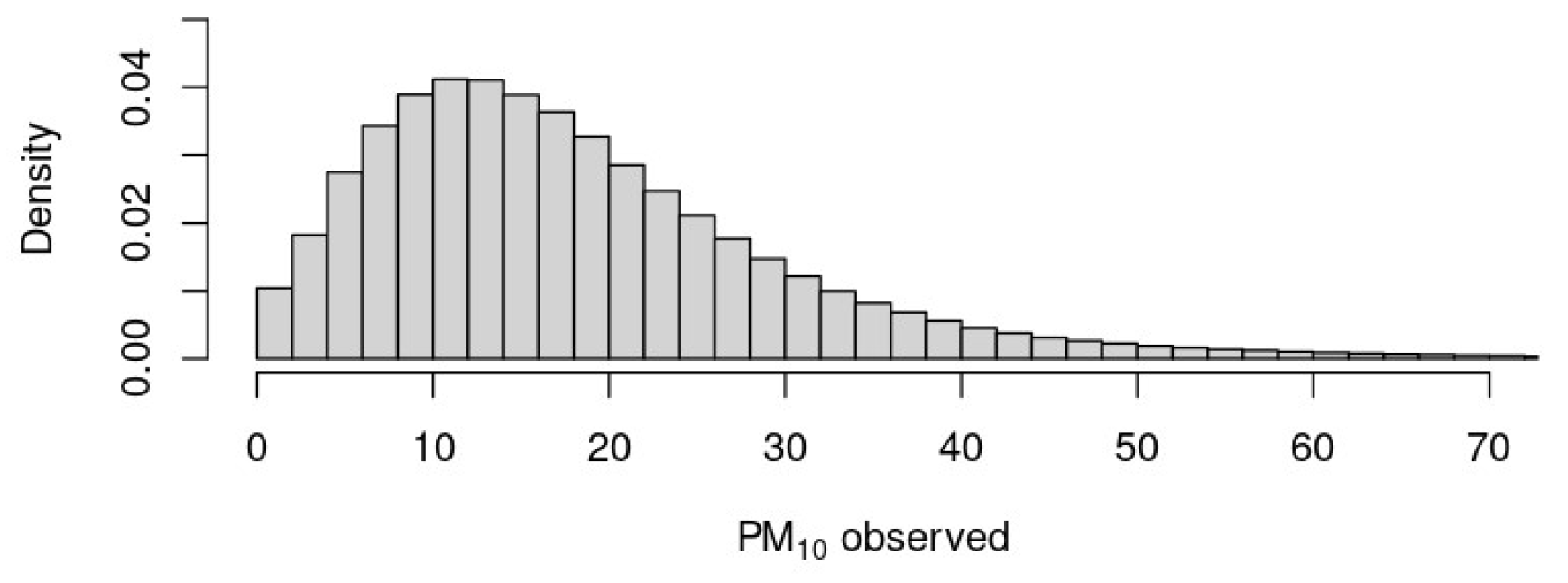
Figure 4 focuses on the value range up to 70 μg m
−3 and demonstrates that overestimation begins at values above approximately 25 μg m
−3. Conversely, in the range from 0 to 25 μg m
−3, there is a systematic overestimation of values. Around 25 μg m
−3, the points align closely with the line of best fit.
Figure 5 provides a histogram of measured PM
10 values corresponding to the Q–Q plot in
Figure 4.
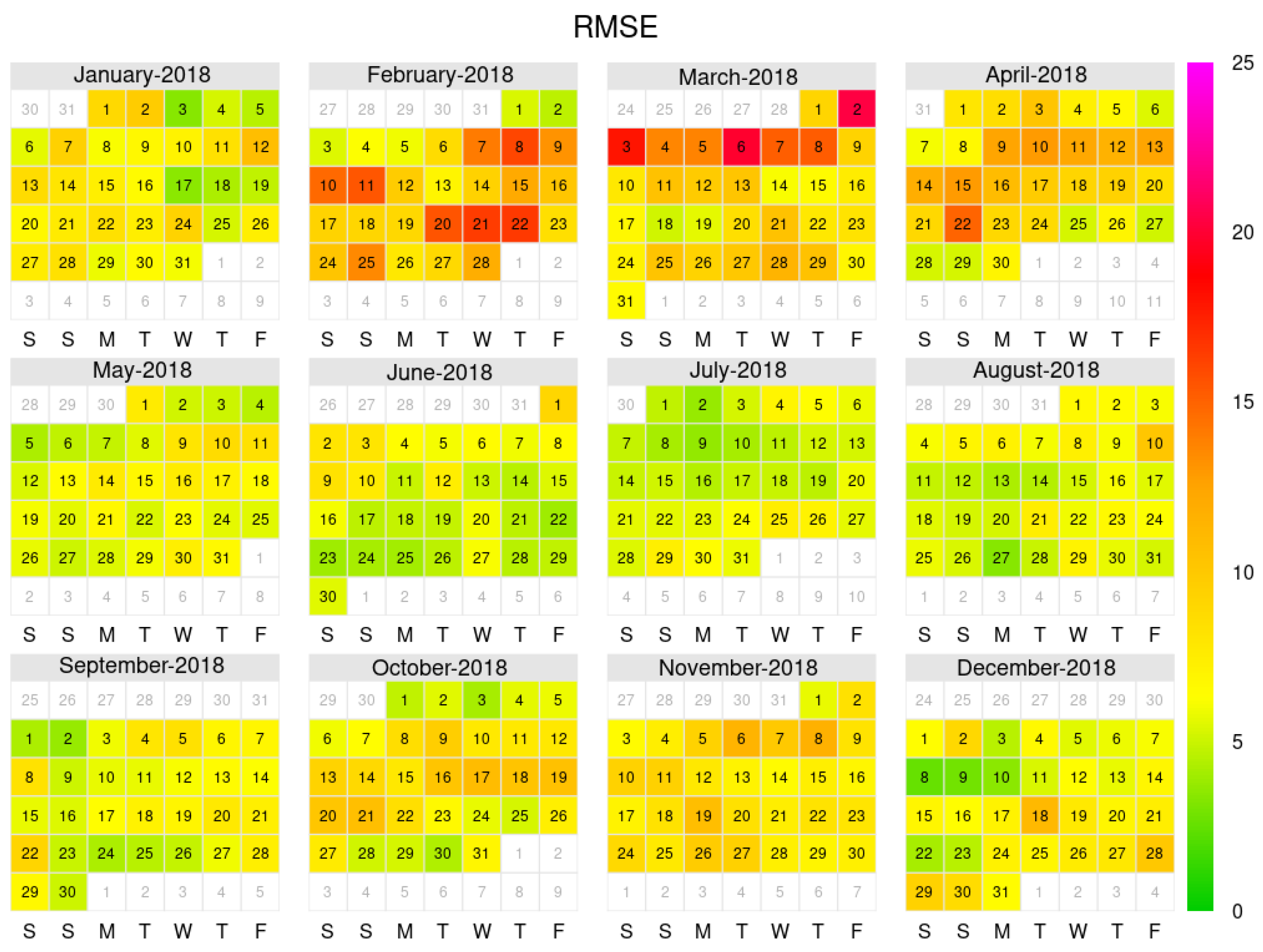
Figure 6 displays the observed PM
10 concentrations in 2018 and exhibits their temporal variations, as reflected in the model performance metric RMSE shown in
Figure 7. The year 2018 was characterised by notably dry conditions, featuring numerous stable high-pressure weather systems, which led to reduced heights of the planetary boundary layer shown in
Figure 8. Additionally, in 2018, several instances occurred where dust originating from the Sahara was transported to Germany.
Excluding days with a Sahara Dust Index (SDI) [
23] greater than 0.4, along with the days immediately preceding and following (due to the singular observation station in Bavaria, Hohenpeißenberg, rendering it non-representative for the entire study area), results in a slight improvement of the error metrics MAE and RMSE, as shown in
Table 3.
The occurrence of several multi-day events posed a challenge, with the model exhibiting underestimation at the onset and overestimation towards the conclusion of such events. These trends are also evident in the calendar plots and apply to the above-mentioned Sahara dust events, which are predicted with a time lag.
Model performance also varies in terms of the classification of the siting type and the surrounding area of the station. The respective values of the evaluation process are shown in
Table 4. As anticipated, model performance is poorer at traffic stations because of the inherently greater magnitude and variability in values. The best evaluation metrics are those from rural background stations, and the worst model performance is observed at industrial stations in urban areas (based on RMSE).
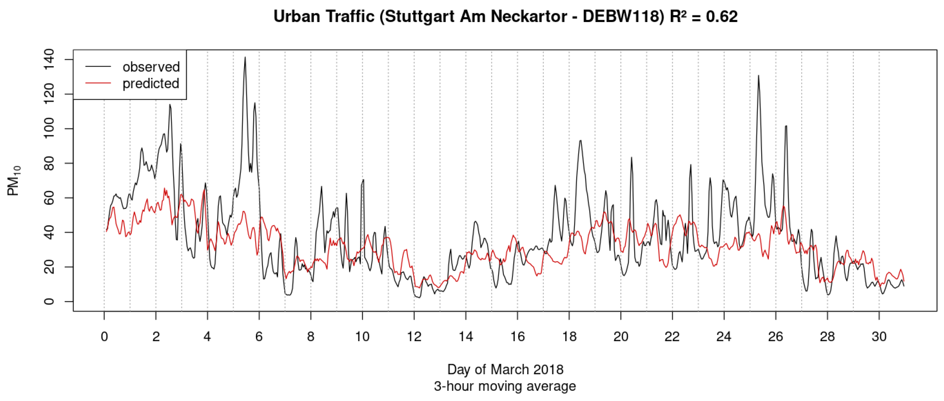
For the month of March 2018, which experienced the highest pollution levels, a separate analysis was conducted for each exemplarily chosen station representing the most frequent combinations of station type and environment. The hourly values were aggregated into rolling 3 h means for better visualisation.
Figure 9,
Figure 10,
Figure 11 and
Figure 12 depict the measured values (black) compared to the modelled values (red).
Representing urban industry, the station in Warstein (DENW181) was selected. The station is situated on a paved area at the eastern edge of the town. Approximately 6 m west lies a two-lane road primarily used as access to quarries. The quarries begin about 400 m southeast of the station and extend south. A federal highway is approximately 450 m from the station. Modelled values often exceed the mostly moderate measured values, exhibiting slight peaks, although the trend of measured values remains relatively constant. Individual events with particularly high concentrations cannot be accurately modelled. The R² value between the measured and modelled values is 0.58.
Similarly, for urban traffic stations, the selected station Stuttgart Am Neckartor (DEBW118) exhibits comparable behaviour. Situated in the capital city of Baden-Württemberg, the station is located on a five-lane (plus one bus lane) road with heavy traffic flow between dense urban development and a green area. Peaks occur more frequently here and are also not accurately reflected by the model. Apart from the peaks, the model follows the general trend of concentration levels throughout the month with an R² of 0.62.
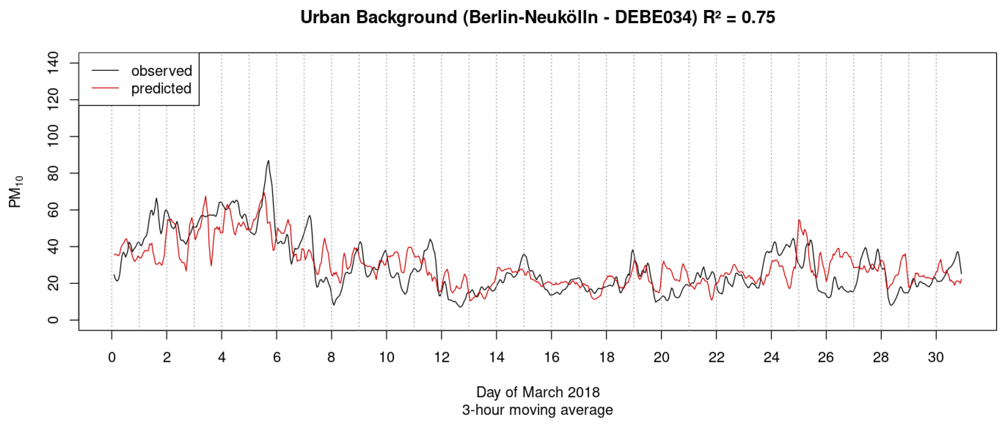
This observation is also evident when considering values for the urban background station Berlin-Neukölln (DEBE034). With few exceptions, the line of modelled values closely follows the line of measured values throughout March 2018, reaching a correlation of R² = 0.75. The measurement station is located in a densely populated residential area in the city centre with moderate traffic flow near a daycare centre.
For the category of rural background, the station Waldhof (DEUB005) was selected. It is located in the eastern part of the Lüneburg Heath on Lower Saxony territory. The nearest settlement is located approximately 3 km to the west. Here, concentrations fluctuate relatively strongly at the beginning of the month, and the model values do not follow those of the measurements. As the month progresses, both values remain mostly low and close to each other. In the last third of the month, the variability of measured concentrations increases again, and the model tends to overestimate them. The correlation of measured and predicted values for this station in March 2018 reaches an R² of 0.68.
The exemplary examination of a selection of representatives for most station-type combinations illustrates the various typical trends and variations for each station type. In most cases, the model could capture these characteristic trends well, achieving correlation coefficients of up to 0.75. However, the peaks that commonly occur at traffic stations could not be captured by the model, resulting in lower coefficients of determination.
The model was not specifically trained to detect exceedances of the currently applicable daily EU-limit value for PM10 of 50 μg m−3. However, for better comparison with similar models, the model’s ability to fulfil this task was still investigated. For this purpose, daily mean concentrations were calculated from the measured and modelled hourly concentration values for all stations in 2018. The model achieved a high accuracy of 98.54%, indicating its overall effectiveness in making correct predictions. However, a closer examination of precision and recall metrics unveiled areas for improvement. While precision was relatively high at 73.96%, suggesting that the model’s positive predictions were generally reliable, the recall value was lower at 27.81%. This indicates that the model might be missing a significant portion of instances where PM10 concentrations exceed the limit value.
4. Discussion
4.1. Sampling
Model training began with a 70/30 train/test split of the entire dataset spanning from 2009 to 2018. The results obtained from this initial setup closely mirrored the outcomes of the internal 5-fold cross-validation performed during the XGBoost training process. However, it is important to note that such a configuration lacks the characteristics of a true forecast model; rather, it operates more as a gap-filling model. In an effort to imbue the model with a more pronounced forecast character, subsequent training sessions utilised data from 2009 to 2017 for training, while the model’s performance was evaluated against data from 2018. This approach yielded the results presented above. However, it is worth mentioning that a rolling-point-forecast model would have been even more optimal in this scenario. It is crucial to acknowledge that samples in the internal 5-fold cross-validation of the model training were not independent, primarily because of the temporal component. The interdependence between samples introduced a certain level of autocorrelation, particularly concerning time-based variables. Ignoring temporal dependencies in time-series data during XGBoost modelling and hyperparameter tuning could lead to violations of assumptions, data leakage, and misleading feature importance. This consideration is essential for understanding the limitations of the model and has to be kept in mind when it comes to validation and application.
4.2. Model Architecture
The model architecture presents opportunities for enhancement through ensemble techniques employing multiple algorithms, which have the potential to increase overall model performance. Additionally, the implementation of one aggregated model for each siting type could mitigate unwanted interference, particularly in cases where stations of different types are in close vicinity. This effect is partly attenuated when coupled with the land use regression model from our previous research [
14], leveraging functions for de-trending and re-trending based on emission/land-use coefficients. Notably, in the context of station-type consideration, urban backgrounds, such as Berlin, exhibit promising performance, likely attributable to the dense network of air monitoring stations in the vicinity. Moreover, the selected meteorological variables contribute significantly to the model, warranting their pre-selection based on expert knowledge. Despite this, metadata such as station latitude and longitude also hold significance, presumed to reflect spatial patterns within the study area.
The importance of the station-type variable ranked last in all preliminary modelling attempts and was subsequently excluded. This could be justified by the fact that the mean concentration of the previous day already implicitly contained this information, as distributions of the measurements follow characteristic patterns depending on the siting type. For example, mean values and measures of dispersion for values from an urban traffic station significantly differ from those of a station in a rural background. The mean PM10 concentration from the preceding day emerges as the most crucial variable, with subsequent days’ concentrations showing diminished importance, possibly because autocorrelation decreases the more time elapses between the points. However, there is potential for refinement in the treatment of this variable; while the model currently considers mean PM10 concentration from one, two, or three days prior, optimisation can involve adjusting the timeframe to better align with predictive accuracy. In the worst case, this value is 23 h apart from the value to be predicted.
The unexpectedly low importance of the variables for cloud cover and precipitation can stem from several factors. Firstly, these variables may be inadequately modelled in the weather model and, hence, in the reanalysis dataset. Additionally, their relatively coarse spatial resolution is a potential limitation. Furthermore, their high correlation with other variables, such as humidity and surface moisture, which are also used and considered more important, can contribute to their diminished importance.
The variable for the hour of the day is also not included in the final model, as it proved to be insignificant in previous iterations. While this may initially seem surprising, it is supported by the weaker diurnal variation compared to the annual cycle observed in PM10 levels. This can also be interpreted as a result of implemented emission reduction measures. Thus, exhaust emissions in Germany have been declining since the mid-1990s and have even fallen below road traffic emissions from abrasion (tyres, brake pads, road surface) since 2015. Unlike gaseous air pollutants, such as NO2, local sources of PM, especially the coarse fraction PM10, contribute less to the overall concentration. Statistically, the low importance of the variable can also be attributed to some meteorological parameters included in the model, such as air temperature, which typically exhibit a relatively strong diurnal pattern.
4.3. Limitations and Improvement Suggestions
The model faces limitations in predicting very high values, primarily because of the mathematical configuration of the algorithm and statistical constraints. These constraints stem from the infrequency of occurrence of such high values, resulting in insufficient data points for effective learning. While attempts were made to address this issue through bias correction using quantile mapping, these efforts proved challenging as only a few values were affected, leading to a limitation in the narrower sense. In evaluating the model’s performance, considerations of accuracy, precision, and recall for limit exceedances are essential. It was observed that in cases of incorrectly identified limit exceedances, measured values mostly hovered just above the threshold, while modelled values of unrecorded exceedances ranged from 30 with increasing density up to the limit of 50, as shown in
Figure 13. In some cases, even with a significant exceedance of the daily limit value, this exceedance was not accurately captured by the model. The study of Feng et al. [
13] achieved values for accuracy and precision of >87% and >86%, respectively. Our model’s accuracy of 98.54% also lies above 87%, but the precision of 73.96% is close to but still below 86%. The reason for this could be that this model was not explicitly trained for this task but rather aims to predict an hourly mean value using regression. It may be possible to improve the model for this purpose by training a classification model for daily mean values instead.
Moreover, the model was unable to accurately capture situations originating entirely outside the study area, such as Sahara dust episodes or long-range transboundary transport of air pollution originating from sources like heating and coal power plants, e.g., in Poland or the Czech Republic. Those impacts could be partially covered by taking into account the wind direction, which varies depending on the season of the year, as shown in
Figure 14. Pültz et al. [
24] investigated the source attribution of particulate matter in Berlin and found that about one-third of the foreign shares can be attributed to Germany’s neighbouring countries Poland and the Czech Republic. However, these contributions can differ significantly during episodes. A potential avenue for improvement involves integrating complementary models like the Copernicus Atmosphere Monitoring Service (CAMS) to learn from errors between models, offering a straightforward yet effective approach. Furthermore, the inclusion of variables from land use regression, traffic, building density, green area, or noise alongside meteorological and time variables can enhance predictive capabilities.
The model demonstrates effectiveness in predicting particulate matter concentrations and may be adaptable for finer fractions of particulate matter. However, caution must be exercised when adapting the model for gaseous contaminants, as their behaviour differs significantly. Additionally, the training and execution of the model are highly cost-, data-, and energy-efficient compared to chemical transport models, aligning with the principles of Green IT and meeting certain environmental requirements.
4.4. Outlook and Further Research Directions
The methodology outlined in
Section 2.3 is optimised for maximising predictive accuracy. However, compared to a classical statistical model not tailored to enhance our comprehension of feature influences on particulate matter concentration, it may lack transparency in attributing specific contributions to results. If a deeper understanding of feature effects was the objective, employing an experimental design enabling statistical tests alongside a more interpretable statistical approach, such as a generalised additive model, would be advisable.
Nevertheless, understanding feature importance remains crucial for comprehending the inner workings of the model and assessing whether our knowledge of influences on the response variable aligns with model attributions. The feature importance illustrated in
Figure 2 is quantified using gain, as originally proposed by Breiman [
25], which evaluates the data homogeneity of child nodes compared to their parent node in a decision tree. However, despite its widespread use, this method can exhibit inconsistency, as demonstrated by Lundberg et al. [
26]. For instance, a feature’s reliance within the model may increase even as its importance decreases. This discrepancy arises because early splits in decision trees, being more crucial, tend to be weighted higher, while gain favours later splits, reflecting a bias inherent in the greedy construction of decision trees. This theoretical limitation persists in tree ensembles like XGBoost.
Theoretically superior methods for measuring feature importance include permutation importance and SHAP (SHapley Additive exPlanations) importance, as defined by Lundberg and Lee [
27]. These methods offer consistency and align closely with human intuition regarding the significance of features [
26]. The SHAP importance for the trained XGBoost model described in
Section 3 is visualised in
Figure 15. While the feature ranking closely resembles the gain-based feature importance depicted in
Figure 2, notable differences arise: the contribution of the previous day’s value appears to have been overestimated in the gain-based importance, while the influence of variables such as the height of the planetary boundary layer and temperature is more pronounced.
Furthermore, SHAP values, the basis for SHAP importance, offer deeper insights by providing feature contributions for each observation. These values, being directional, allow visualisation of not only the magnitude but also the direction of feature contributions; for instance, small values in a feature may correspond to increased values in the target. Additionally, we can visualise the impact of a single feature through dependence plots or for a single observation using waterfall plots, elucidating how each feature contributes to the prediction.
A promising extension is transitioning from point forecasts to probabilistic forecasts, increasingly popular in weather forecasting, as discussed in works such as Gneiting and Katzfuss [
28] and Scheuerer and Hamill [
29]. This shift offers several benefits, including deeper insights into differences between stations or over time, the quantification of uncertainty through confidence intervals, and the ability to generate varying point forecasts without retraining by retrieving percentiles and expectiles from the distribution. A straightforward approach involves selecting a suitable distribution and forecasting its parameters, as demonstrated in the XGBoostLSS algorithm by März and Kneib [
30], which builds upon the standard XGBoost library. Alternatively, more flexible options, such as transformation forests, as explored by Schlosser et al. [
31], offer probabilistic forecasting without pre-defining a distribution.


 ,
, 


