Seasonality of Heavy Metal Concentrations in Ambient Particulate Matter in the UK

Abstract

The seasonal characteristics of air pollutant concentrations are important for understanding variations in emissions released into the air and in atmospheric chemistry. The patterns seen can be influenced by anthropogenic emissions, meteorological conditions, and the transport of pollutants over long and short distances. Whilst seasonality is well understood for some pollutants such as ozone and polycyclic aromatic hydrocarbons, it is poorly understood and under-investigated for heavy metals in particulate matter (PM). This work studies long-term datasets of heavy metals in PM from a relevant UK air quality monitoring network, demonstrating the seasonal characteristics of the concentrations of these metals for the first time. Surprisingly, both ‘high in winter–low in summer’ and ‘low in winter–high in summer’ seasonality was observed, with some metals showing little or no seasonality. The ‘high in winter–low in summer’ seasonality (particularly for As) is attributable to the dominant contribution being from local primary sources, such as burning process producing larger PM sizes. The ‘low in winter–high in summer’ seasonality (particularly for V) is attributable to weak or non-seasonal local sources being dominated by contributions from medium and long-range transport during the summer months, when pollutant transport is more efficient. The findings contribute significantly to our understanding of the seasonality of metals in PM concentrations and the role played by the long-range transport of pollutants. Conclusions are also drawn about the implications for the calculation of annual averages on compliance-based air quality networks if data from a time series of a pollutant that displays seasonal characteristics are missing.

1. Introduction

Ambient air pollution has a major effect on human health, causing an estimated 29,000–43,000 deaths per year in the UK [1]. Exposure to particles, particularly those with an aerodynamic diameter of less than 2.5 μm (PM_2.5), over both a long and short term has been shown to have significant detrimental effects on human health [2]. Understanding the composition of these particles helps to reveal in more detail the mechanisms by which negative health outcomes arise. In particular, heavy metals in ambient particulate matter are known to cause diseases and adverse health conditions [3,4], such as cardiovascular disease, pulmonary illnesses, cancer, and central nervous system disorders [5]. UK legislation has set an annual average limit value for Pb concentrations in air of 500 ng m⁻³ [6] and annual average target values for As, Cd, and Ni concentrations in air [7] of 6 ng m⁻³, 5 ng m⁻³, and 20 ng m⁻³, respectively. These and other heavy metal concentrations are monitored by many national networks across the globe, such as the UK Heavy Metals Network [8].

Measured concentrations at a given air quality monitoring station are dependent on both local emissions and the effects of long-range transport. Examining the seasonality of heavy metal concentrations can provide information on the pollution climate and possible emission sources [9,10,11,12,13,14] that impact particular monitoring stations. The emission rates of different heavy metals throughout a year depend on the specific processes producing them. For example, the emissions of heavy metals from fuel used for heating will be higher in the colder months and lower in the warmer months. However, emissions from industry and transport are far more likely to be constant throughout a year, unless there is a seasonality component of production or travel intensity. Analysing the seasonality of metal concentrations can not only identify these contributions but also provide information on whether short-range or long-range transport is dominant. Seasonal concentration effects are well known for other air pollutants such as ozone or polycyclic aromatic hydrocarbons (PAH) in PM [15], which are dominated by seasonal weather (in the case of ozone) and seasonal emissions (in the case of PAHs). However, work in the literature examining and identifying these effects for metals in PM has been rare, with some studies observing seasonality in Asia and South America [16,17,18,19]. To the best of the authors’ knowledge, no such systematic studies have been undertaken in the UK, perhaps because it has generally been assumed that emission sources producing metals are constant throughout the year and prevailing weather has no effect [20], so seasonal effects are likely to be small. As a result, a casual examination of metal concentrations usually fails to yield clear seasonality, and more careful data analysis techniques applied over a multi-year time frame, as used in this work, are required to tease out any underlying seasonality.

2. Materials and Methods

2.1. Monitoring Stations and Sample Analysis

Measurements made by the UK Heavy Metals Air Quality Monitoring Network (‘the Network’) were used in this study. This Network, which is operated by the National Physical Laboratory on behalf of the Environmental Agency and the UK Department for Environment, Food, and Rural Affairs, consists of 24 monitoring stations making measurements across the UK, with 23 of these stations collecting weekly PM₁₀ samples onto cellulose ester filters using samplers with a flow rate of 1 m³ h⁻¹ and with each filter being exposed for a one-week period. (This network samples only PM₁₀, as required by regulations for heavy metals in PM, so no information was available on other size fractions such as PM_2.5. Furthermore, detailed information about the local weather and wind profiles close to the monitoring stations was also not available for this study.) Depending on monitoring station location and local dominant industrial emissions, weekly filters are either analysed individually or bulked together to provide four-weekly results. Filters are microwave-digested in a mixture of hydrogen peroxide and nitric acid and then analysed using Inductively Coupled Plasma Mass-Spectrometry (ICP-MS) via the method specified in BS EN 14902 [21] and independently accredited to ISO 17025 [22]. A full description of the Network, a map of its monitoring stations, a description of its operation, the quality assurance measures taken, and the independently accredited analysis techniques used have been provided previously [23]. (A map of the monitoring stations on this Network may also be found at https://uk-air.defra.gov.uk/interactive-map?network=metals, accessed on 22 May 2024.) The metals considered in this study were Zn, V, Cr, Cu, Ni, As, Mn, Pb, Cd, Fe, Co, and Se as they return concentrations above the detection limit for the vast majority of samples, giving more confidence in any conclusions drawn based on concentration trends. Between 2005 and 2010, the UK Heavy Metals Network established more monitoring locations to provide better coverage of emissions from industrial sources. These stations have mostly been monitoring continuously ever since, making the network well suited to providing a long-term dataset from around 2005 onwards. Importantly, analysing a long-term dataset helps to average out any outliers caused by short-term meteorological events and, taken together with the other steps taken during the data analysis stage (see below), enables seasonality effects to be deconvolved with confidence. Therefore, these monitoring stations were chosen as they are the only locations in the UK at which metals in PM₁₀ have been routinely measured for a sufficiently long time period to be of use for detecting seasonality.

Table 1. Monitoring station, location, station type and the period data were selected for use in this study. (* The Sheffield Centre monitoring station was relocated to Sheffield Devonshire Green in 2013. In this analysis, these two monitoring stations are considered to produce the same, continuous dataset due to their immediate neighbouring geographical locations.)

Monitoring Station	Data Used from	Data Used to	Latitude	Longitude	Country	Type
Belfast Centre	01/01/2010	31/12/2022	54.59965	−5.92883	Northern Ireland	Urban Background
Chadwell St Mary	01/01/2010	31/12/2022	51.48196	0.37021	England	Urban Background
Cromwell Road	01/01/2005	31/12/2013	51.49548	−0.17871	England	Urban Traffic
Eskdalemuir	01/01/2005	31/12/2022	55.31531	−3.20611	Scotland	Rural Background
London Marylebone Road	01/04/2011	31/12/2022	51.52253	−0.15461	England	Urban Traffic
London Westminster	01/01/2005	31/12/2022	51.49467	−0.13193	England	Urban Background
Pontardawe Brecon Road	11/08/2011	31/12/2022	51.72651	−3.84344	Wales	Suburban Industrial
Pontardawe Tawe Terrace	01/01/2011	31/12/2022	51.72001	−3.84722	Wales	Urban Industrial
Port Talbot Margam	01/01/2010	31/12/2022	51.58395	−3.77082	Wales	Urban Industrial
Scunthorpe Low Santon	01/01/2010	31/12/2022	53.59583	−0.59724	England	Suburban Industrial
Scunthorpe Town	01/01/2010	31/12/2022	53.58634	−0.63681	England	Urban Industrial
Sheffield Devonshire Green *	01/01/2010	31/12/2022	53.37862	−1.47810	England	Urban Background
Swansea Coedgwilym	01/01/2010	31/12/2022	51.70168	−3.87401	Wales	Urban Background
Swansea Morriston	01/01/2010	31/12/2022	51.66212	−3.92130	Wales	Urban Traffic
Walsall Bilston Lane	01/01/2005	29/08/2018	52.58313	−2.04280	England	Urban Industrial

shows the monitoring stations used to provide concentration data for this study, along with the monitoring period considered and station location and type. The station type is provided in accordance with the 4th EU Directive on Air Quality requirements for macroscale siting [24]. In most cases, the ‘industrial’ designation will only relate to the emissions of one metal from a nearby industrial source and will likely not apply to all of the metals studied in this work.

2.2. Data Processing and Analysis

The aim of this study was to investigate the seasonality of measured heavy metal concentrations in PM₁₀ in the UK. Given the availability of data and the need to compare the same time interval across different years, this goal is most easily achievable on a calendar-month basis. However, given that sampling periods usually spanned the boundary between calendar months and that some data were available on a weekly basis whilst some were only available on a four-weekly basis, the weighting of all data had to be equalised. To achieve this, the weekly or four-weekly concentration of each measurement was assigned to each day covering the relevant sample period. For example, in the case of a filter sampled from 1 February 2019 to 28 February 2019 the average measured concentration was taken to be 28 identical daily concentrations covering this period. Similarly, concentrations from weekly samples became seven identical daily concentrations. From this, calendar month concentrations could easily be calculated as the simple mean of the concentrations attributed to the days within a particular calendar month.

Annual means for each heavy metal at each monitoring station were then calculated from these daily concentrations within the relevant calendar year. Each day’s concentration was then normalised by dividing by the relevant annual mean for said day. This was performed so that data from different years could be compared with confidence and without the biasing effect of mean annual concentrations generally decreasing steadily over the period studied [23]. Without normalisation to each year’s mean, this background trend would have masked any seasonality in concentrations. Then, the median of the normalised concentrations for each calendar month throughout the multi-year sampling period was then calculated for each heavy metal and station combination. This produced 12 values for each heavy metal and station combination, one for each month. For each metal, quadratic fitting was then performed (using the Microsoft Excel software package, version 2308) on these 12 median values arranged in equally spaced month order from January to December on the x-axis (with January designated as ‘1’, February designated as ‘2’, and so on through to December, which was designated as ‘12’). There are no physical models specifically underpinning a quadratic relationship—the model used is purely empirical—but similar models have previously been used to successfully characterise seasonality in pollutant concentrations [15], and the quadratic fitting coefficient (referred to as the ‘x² coefficient’, which is equal to ‘a’ in the fitted quadratic relationship y = ax² + bx + c) produced allows meaningful comparison across the different datasets. The x² coefficient resulting from the quadratic fit was used as an empirical indication of the strength of any seasonality effect observed. A positive x² coefficient indicates that concentrations are higher at the start and end of a year than during the middle months. In contrast, a negative x² coefficient indicates that mid-year concentrations are higher than those at the start and end of a year. The coefficient of determination, R², was used to indicate the proportion of the variation in the dependent variable that was attributable to a quadratic relationship. The closer the R² value is to 1, the greater the proportion of variation in the dependent variable that is attributable to a quadratic relationship, which implies a stronger relationship, sometimes also referred to as ‘goodness of fit’. The statistical approach chosen was highly suitable for this study as it allows data obtained in different sampling periods—spanning across calendar months and years, with a background trend of decreasing overall concentrations—to be effectively and robustly analysed for small seasonality effects. Other time series analysis techniques would not have been suitable or would have lacked the sensitivity required.

Due to significantly higher-than-average, outlying concentrations being observed during annual events in the UK characterised by bonfires and fireworks on and around Bonfire Night (5 November, in mainland UK) and Eleventh Night (11 July, in Northern Ireland), the dataset was also analysed with filters (and therefore concentration values) covering the periods being excluded lest they obfuscate the seasonality trends. (These data are not ‘outliers’ as such since they are real measured values. However, they are ‘outlying’ in terms of the overall shape of the seasonality observed.)

3. Results and Discussion

Table 2. (a) The x² coefficient from the quadratic fits for the median annual seasonal profile at each monitoring station and for As, Pb, Zn, Cd, Cu, and Fe, and the associated R² values for the complete dataset, sorted in descending order of the x² coefficient. Key to the colours for x²: green—when x² > 0.01; orange—when 0.01 ≥ x² ≥ 0; red—when 0 > x². Key to the colours for R²: green—when R² > 0.6; orange—when 0.6 ≥ R² ≥ 0.4; red—when 0.4 > R². (b) The x² coefficient from the quadratic fits for the median annual seasonal profile at each monitoring station and for Cr, Co, Se, Ni, Mn and V, and the associated R² values for the complete dataset, sorted in descending order of the x² coefficient. Key to the colours for x²: green—when x² > 0.01; orange—when 0.01 ≥ x² ≥ 0; red—when 0 > x². Key to the colours for R²: green—when R² > 0.6; orange—when 0.6 ≥ R² ≥ 0.4; red—when 0.4 > R².

(a)
Monitoring Station	As		Pb		Zn		Cd		Cu		Fe
	x2	R2	x2	R2	x2	R2	x2	R2	x2	R2	x2	R2
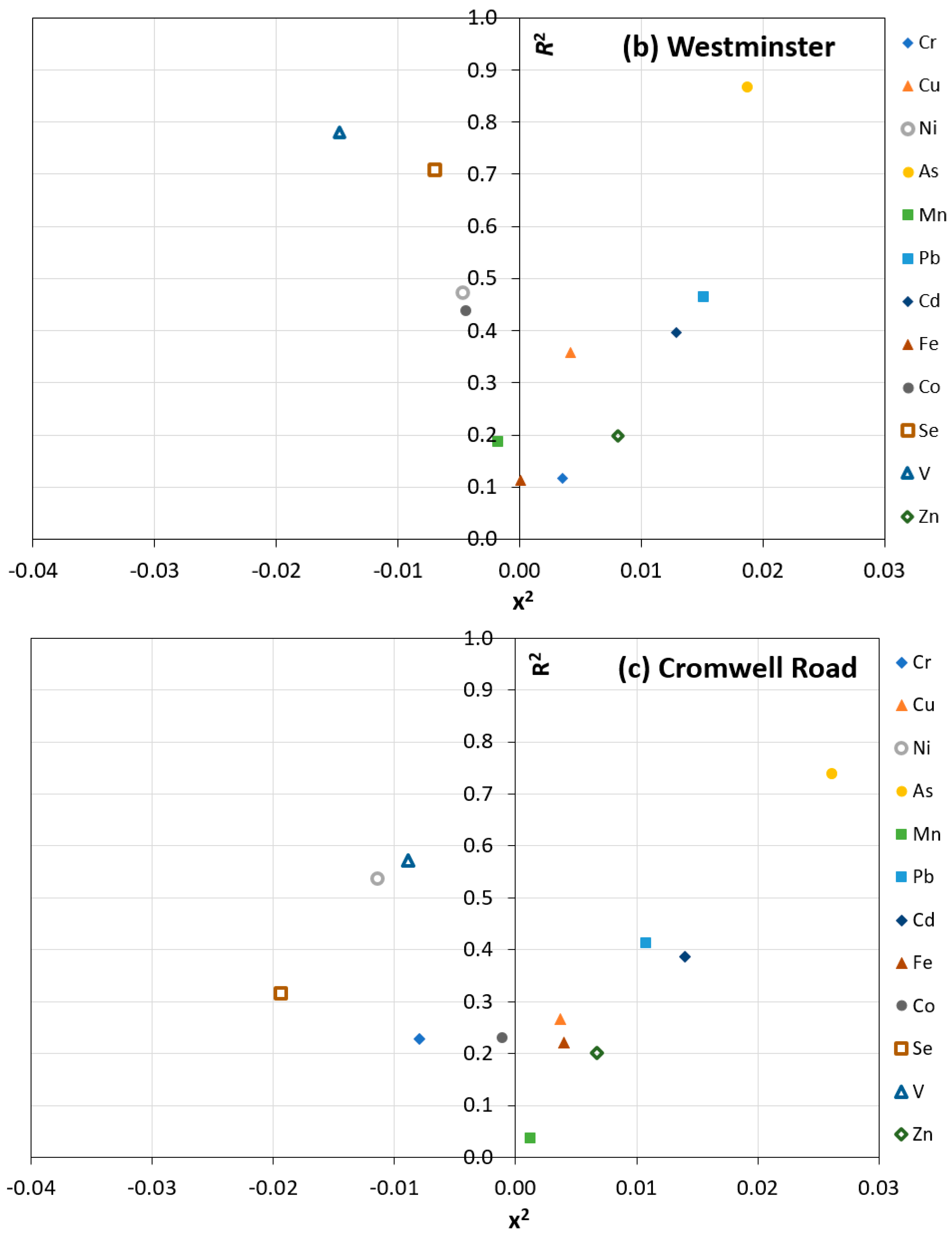
Cromwell Road	0.0253	0.556	0.0122	0.469	0.0058	0.164	0.0128	0.349	0.0028	0.214	0.0030	0.260
Pontardawe Tawe Terrace	0.0211	0.770	0.0084	0.439	0.0039	0.204	−0.0061	0.234	0.0105	0.599	0.0034	0.080
Walsall Bilston Lane	0.0192	0.555	0.0136	0.609	0.0132	0.576	0.0095	0.417	0.0099	0.453	0.0000	0.338
Westminster	0.0190	0.689	0.0119	0.585	0.0082	0.213	0.0107	0.363	0.0042	0.334	−0.0008	0.068
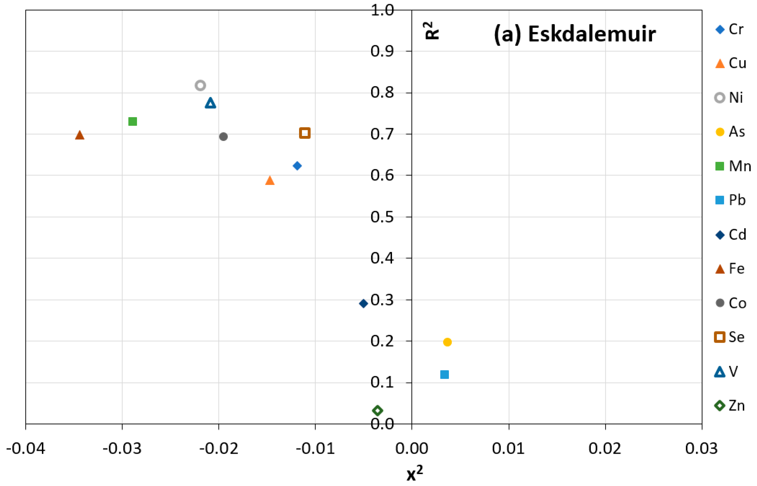
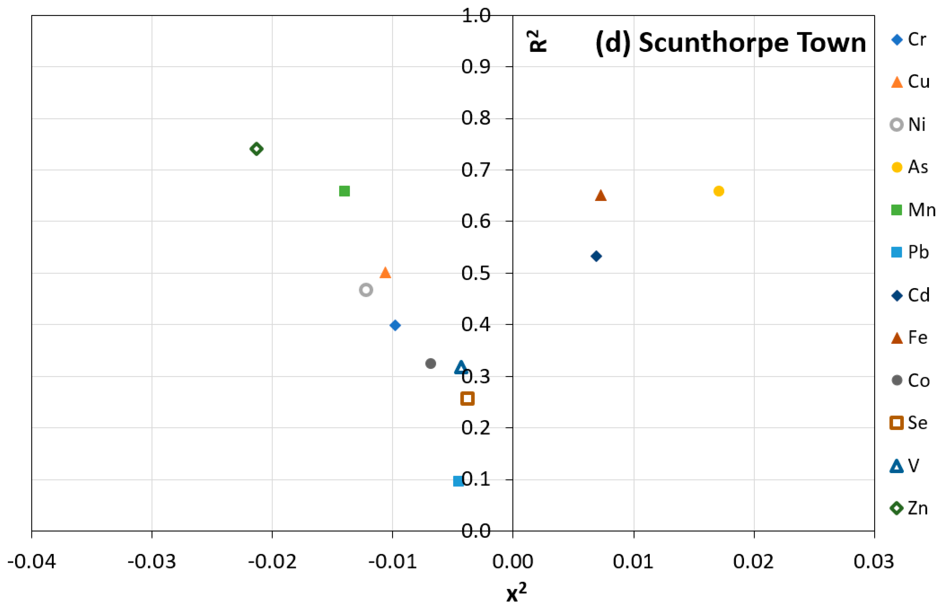
Scunthorpe Town	0.0174	0.472	−0.0051	0.168	−0.0213	0.818	0.0070	0.221	−0.0107	0.448	0.0107	0.437
Swansea Coedgwilym	0.0173	0.676	0.0136	0.659	0.0009	0.019	−0.0014	0.079	0.0101	0.736	−0.0023	0.083
Scunthorpe Low Santon	0.0164	0.616	0.0060	0.250	0.0084	0.369	0.0053	0.217	0.0061	0.323	0.0020	0.138
Pontardawe Brecon Road	0.0154	0.762	0.0091	0.239	0.0001	0.106	−0.0037	0.082	0.0020	0.403	−0.0011	0.052
Chadwell St Mary	0.0140	0.371	0.0096	0.443	0.0062	0.222	0.0067	0.269	0.0085	0.387	−0.0009	0.068
Sheffield Devonshire	0.0139	0.413	0.0093	0.228	0.0028	0.087	0.0031	0.024	0.0091	0.499	−0.0008	0.027
Marylebone Road	0.0139	0.589	0.0090	0.372	0.0031	0.155	0.0073	0.266	−0.0039	0.536	−0.0018	0.456
Swansea Morriston	0.0103	0.263	0.0058	0.305	0.0029	0.216	0.0000	0.266	0.0078	0.720	0.0081	0.541
Port Talbot	0.0093	0.613	−0.0075	0.535	0.0071	0.704	−0.0076	0.324	−0.0022	0.495	−0.0196	0.602
Belfast Centre	0.0067	0.182	−0.0045	0.038	−0.0188	0.192	−0.0008	0.004	0.0045	0.433	−0.0038	0.153
Eskdalemuir	0.0054	0.165	0.0048	0.070	−0.0003	0.005	−0.0060	0.243	−0.0135	0.549	−0.0361	0.699
(b)
Monitoring Station	Cr		Co		Se		Ni		Mn		V
	x2	R2	x2	R2	x2	R2	x2	R2	x2	R2	x2	R2
Cromwell Road	−0.0087	0.264	−0.0005	0.034	−0.0202	0.291	−0.0134	0.603	−0.0002	0.075	−0.0108	0.661
Pontardawe Tawe Terrace	−0.0022	0.023	−0.0048	0.156	−0.0069	0.724	−0.0084	0.348	−0.0075	0.305	−0.0162	0.675
Walsall Bilston Lane	−0.0036	0.043	−0.0002	0.007	−0.0032	0.184	0.0033	0.392	0.0047	0.133	−0.0058	0.341
Westminster	0.0035	0.126	−0.0035	0.315	−0.0068	0.665	−0.0048	0.642	−0.0025	0.227	−0.0158	0.772
Scunthorpe Town	−0.0083	0.437	−0.0073	0.478	−0.0032	0.301	−0.0142	0.684	−0.0156	0.794	−0.0055	0.329
Swansea Coedgwilym	0.0081	0.657	0.0112	0.703	−0.0047	0.740	0.0091	0.482	−0.0092	0.273	−0.0152	0.728
Scunthorpe Low Santon	−0.0113	0.477	−0.0002	0.032	0.0052	0.221	−0.0023	0.085	−0.0150	0.575	−0.0200	0.777
Pontardawe Brecon Road	0.0003	0.094	0.0010	0.155	−0.0056	0.546	0.0066	0.669	−0.0090	0.352	−0.0144	0.745
Chadwell St Mary	−0.0007	0.106	−0.0073	0.383	−0.0098	0.646	−0.0065	0.510	−0.0059	0.476	−0.0139	0.742
Sheffield Devonshire	−0.0042	0.422	−0.0028	0.235	−0.0088	0.229	0.0018	0.424	−0.0092	0.548	−0.0102	0.478
Marylebone Road	−0.0021	0.327	−0.0023	0.256	−0.0056	0.347	−0.0081	0.693	−0.0030	0.553	−0.0145	0.735
Swansea Morriston	0.0057	0.364	−0.0052	0.169	−0.0070	0.836	0.0016	0.097	0.0015	0.032	−0.0115	0.581
Port Talbot	−0.0057	0.186	−0.0116	0.506	−0.0079	0.689	−0.0072	0.553	−0.0193	0.696	−0.0265	0.735
Belfast Centre	−0.0059	0.100	−0.0173	0.743	0.0021	0.116	−0.0297	0.848	−0.0077	0.415	−0.0328	0.706
Eskdalemuir	−0.0106	0.654	−0.0206	0.697	−0.0111	0.685	−0.0239	0.801	−0.0294	0.723	−0.0230	0.823

a,b and

Table 3. (a) The x² coefficient from the quadratic fits for the median annual seasonal profile at each monitoring station and for As, Pb, Zn, Cd, Cu, and Fe, and the associated R² values for the dataset with the effect of bonfire events removed, sorted in descending order of the x² coefficient. Key to the colours for x²: green—when x² > 0.01; orange—when 0.01 ≥ x² ≥ 0; red—when 0 > x². Key to the colours for R²: green—when R² > 0.6; orange—when 0.6 ≥ R² ≥ 0.4; red—when 0.4 > R². (b) The x² coefficient from the quadratic fits for the median annual seasonal profile at each monitoring station and for Cr, Co, Se, Ni, Mn, and V, and the associated R² values for the dataset with the effect of bonfire events removed, sorted in descending order of the x² coefficient. Key to the colours for x²: green—when x² > 0.01; orange—when 0.01 ≥ x² ≥ 0; red—when 0 > x². Key to the colours for R²: green—when R² > 0.6; orange—when 0.6 ≥ R² ≥ 0.4; red—when 0.4 > R².

(a)
Monitoring Station	As		Pb		Zn		Cd		Cu		Fe
	x2	R2	x2	R2	x2	R2	x2	R2	x2	R2	x2	R2
Cromwell Road	0.0261	0.738	0.0108	0.413	0.0067	0.201	0.0140	0.386	0.0037	0.266	0.0040	0.221
Pontardawe Tawe Terrace	0.0201	0.837	0.0088	0.572	0.0033	0.291	−0.0071	0.329	0.0094	0.618	0.0029	0.062
Westminster	0.0187	0.868	0.0151	0.465	0.0081	0.198	0.0129	0.397	0.0042	0.357	0.0001	0.112
Walsall Bilston Lane	0.0171	0.616	0.0113	0.308	0.0110	0.428	0.0053	0.083	0.0078	0.226	−0.0006	0.245
Scunthorpe Town	0.0171	0.659	−0.0045	0.096	−0.0213	0.741	0.0069	0.533	−0.0106	0.501	0.0073	0.652
Swansea Coedgwilym	0.0152	0.653	0.0134	0.661	−0.0008	0.082	−0.0019	0.160	0.0093	0.714	−0.0024	0.080
Scunthorpe Low Santon	0.0150	0.734	0.0039	0.248	0.0070	0.360	0.0028	0.153	0.0040	0.195	0.0019	0.211
Belfast Centre	0.0144	0.648	0.0032	0.053	−0.0056	0.446	0.0067	0.238	0.0036	0.422	−0.0058	0.321
Marylebone Road	0.0142	0.716	0.0050	0.340	0.0026	0.122	0.0080	0.322	−0.0047	0.493	−0.0030	0.466
Pontardawe Brecon Road	0.0134	0.754	0.0083	0.253	−0.0007	0.140	−0.0049	0.197	0.0018	0.433	−0.0014	0.038
Chadwell St Mary	0.0134	0.498	0.0111	0.608	0.0059	0.242	0.0057	0.359	0.0077	0.456	−0.0009	0.114
Sheffield Devonshire	0.0124	0.469	0.0076	0.323	−0.0013	0.303	0.0007	0.236	0.0076	0.524	−0.0014	0.102
Swansea Morriston	0.0092	0.291	0.0045	0.347	0.0028	0.301	−0.0030	0.473	0.0066	0.722	0.0090	0.522
Port Talbot	0.0089	0.599	−0.0086	0.626	0.0060	0.429	−0.0080	0.262	−0.0039	0.462	−0.0196	0.602
Eskdalemuir	0.0037	0.197	0.0034	0.119	−0.0036	0.032	−0.0050	0.290	−0.0147	0.588	−0.0344	0.699
(b)
Monitoring Station	Cr		Co		Se		Ni		Mn		V
	x2	R2	x2	R2	x2	R2	x2	R2	x2	R2	x2	R2
Cromwell Road	−0.0079	0.229	−0.0011	0.230	−0.0194	0.316	−0.0114	0.538	0.0012	0.036	−0.0089	0.571
Pontardawe Tawe Terrace	−0.0027	0.035	−0.0035	0.133	−0.0069	0.673	−0.0084	0.349	−0.0076	0.283	−0.0167	0.701
Westminster	0.0035	0.117	−0.0044	0.439	−0.0070	0.709	−0.0047	0.475	−0.0018	0.187	−0.0148	0.780
Walsall Bilston Lane	0.0057	0.117	−0.0015	0.095	−0.0043	0.374	0.0016	0.241	0.0030	0.066	−0.0050	0.348
Scunthorpe Town	−0.0098	0.398	−0.0068	0.324	−0.0038	0.257	−0.0122	0.467	−0.0140	0.658	−0.0043	0.318
Swansea Coedgwilym	0.0084	0.700	0.0116	0.706	−0.0053	0.682	0.0092	0.522	−0.0087	0.236	−0.0149	0.739
Scunthorpe Low Santon	−0.0109	0.431	−0.0010	0.025	0.0063	0.404	−0.0041	0.346	−0.0154	0.556	−0.0195	0.695
Belfast Centre	−0.0086	0.150	−0.0203	0.800	0.0011	0.082	−0.0315	0.796	−0.0084	0.493	−0.0356	0.768
Marylebone Road	−0.0023	0.305	−0.0016	0.251	−0.0049	0.287	−0.0078	0.675	−0.0035	0.437	−0.0149	0.783
Pontardawe Brecon Road	0.0004	0.103	0.0010	0.119	−0.0054	0.560	0.0056	0.441	−0.0096	0.405	−0.0138	0.712
Chadwell St Mary	−0.0042	0.075	−0.0083	0.525	−0.0093	0.652	−0.0059	0.408	−0.0058	0.474	−0.0138	0.768
Sheffield Devonshire	−0.0042	0.431	−0.0041	0.245	−0.0096	0.219	0.0011	0.491	−0.0092	0.571	−0.0103	0.507
Swansea Morriston	0.0061	0.362	−0.0042	0.160	−0.0070	0.823	0.0018	0.089	0.0021	0.033	−0.0114	0.584
Port Talbot	−0.0065	0.278	−0.0122	0.516	−0.0083	0.613	−0.0076	0.586	−0.0190	0.748	−0.0262	0.735
Eskdalemuir	−0.0119	0.623	−0.0195	0.693	−0.0111	0.703	−0.0219	0.817	−0.0289	0.729	−0.0209	0.776

a,b show the x² coefficient from the quadratic fits and the associated R² values for the complete dataset and the same dataset with the effect of bonfires removed, respectively. As a guide for the eye, the table cells have been colour-coded to show the strength of the seasonality and goodness of fit, with the table key describing the colouring criteria. The threshold values for x² are arbitrary values; however, an R² greater than 0.6 for 10 degrees of freedom (12 datapoints) exceeds the critical value for a probability of 95% in a 2-tailed test. The other two bandings for R² are arbitrary.

In Table 2a,b, it can be seen that the As data show a positive x² coefficient for all monitoring stations, with the coefficient decreasing in strength from Cromwell Road down to Eskdalemuir. Removing the bonfire periods (Table 3a,b) has little effect on the x² coefficient at all stations except Belfast Centre; however, it improves the ‘goodness of fit’ at 11 of the 14 stations and leads to an average improvement of 0.11. Belfast exhibits a large change in the strength of the x² term and an improvement in R², as the bonfires occur in July in Northern Ireland, while they occur in November in Great Britain. Figure 1 shows the seasonality for As at London Westminster for both datasets and the clear drop in November concentrations once bonfire periods have been removed.

The seasonality at London Westminster is likely to be caused by seasonality in combustion emissions. Over this period, the As emissions from the open burning of treated wood were constant [25], with this emission source contributing 63% of As emissions in 2021.

In contrast to Figure 1, Figure 2 shows the weak seasonality in As concentrations at Eskdalemuir, which, as a rural background location, is subject to no strong local sources.

The data in Table 3 may also be displayed as a scatter plot of the x² coefficient on the x-axis against the coefficient of determination, R², on the y-axis. This is shown in Figure 3.

Figure 3 clearly shows the range of seasonality displayed by different metals and how this varies depending on the monitoring station. For example, As shows positive seasonality with generally good correlations at all monitoring stations, whilst V shows negative seasonality with generally good correlations at all monitoring stations. Other metals, such as Cu and Cd, show a mixture of positive and negative seasonality depending on the monitoring station, generally exhibiting poorer correlations. This demonstrates, for the first time, the seasonality of the concentration of heavy metals in PM₁₀ in the UK. Some metals show positive seasonality (high in winter–low in summer), as seen for other pollutants whose emissions are dominated by local burning processes. However, some metals showed negative seasonality (low in winter–high in summer), which is more surprising. This is the first time this inverse seasonality behaviour has been observed in relation to metals in the UK, although a few other studies conducted outside the UK have observed this effect. Urban background measurements in Northern China have shown this inverse seasonality for V measurements [9], whilst large-scale modelling of V concentrations in regional East Asia has also shown the same effect [13]. The data displayed in Figure 3 are easier to interpret if each metal is considered individually, since this also allows specific monitoring stations to be attributed to each data point. This has been realized in Figure 4.

The literature suggests that the particle size distributions of As emissions are centred around 2 µm, with some studies suggesting sizes up to 5.5 µm [26]. This would indicate that As emissions are not prone to extensive long-range transport. Instead, As in PM₁₀ comes from primary emissions more likely to be dominated by sources local to a given monitoring station, such as burning processes that are more prevalent in the winter than in the summer. Figure 3 demonstrates this, with the majority of monitoring stations showing positive seasonality for As, with a high R² value. The metal with the second strongest positive seasonality is Pb, followed by Zn, although both seasonality results are significantly less pronounced than those for As, with a few monitoring stations also showing negative seasonality for these metals.

V, in contrast to all the other metals, shows negative seasonality for all the monitoring stations, including at rural background and industrial background locations. Figure 5 shows the seasonality for V concentrations measured in Belfast with the effect of bonfires removed (there is little difference in the x² coefficient with and without the effect of bonfires). This negative seasonality is consistent with observations in the literature [9,13] but is believed by the authors to be the first time this has been observed for V in the UK. Figure 6 shows a scatter plot for V similar to that for As in Figure 3.

All the monitoring stations in Figure 6 show a negative x² coefficient, indicating higher V concentrations in warmer months than in colder months. As V is not normally emitted via heating fuels, this would indicate that the V comes from long-range transport—which is more prevalent in warner months—and not local combustion emissions. According to the UK National Atmospheric Emission Inventory (NAEI), petroleum-based fuels (diesel (DERV), fuel oil, gas oil, and petroleum coke) are the main source of V and contributed 90% of the total V emissions in 2021. The use of diesel for road transport accounted for 54% of UK emissions, and V is one of the few metals for which road fuel use is a major source. Emissions from road transport have more than doubled since 1990 due to the increasing use of diesel. If the V concentrations in Belfast predominantly stemmed from local traffic emissions, then pronounced negative seasonality would not be expected, as traffic emissions would be expected to be much more stable throughout the year. It is therefore likely that other, non-local sources play a significant role in contributing to the observed concentrations.

V is known to be present in both crude oil and coal in widely varying concentrations [27]. V in crude oil is concentrated in the heaviest distillation fractions and can reach extremely high concentrations in derived fuels such as residual oil (heavy fuel oil (HFO)) and petroleum coke. In global emission inventories, the presence of V is almost exclusively ascribed to the combustion of heavy petroleum products. However, international shipping emissions (defined by voyage origin and destination, not ship registration) are not included in a country’s emission inventory and are reported separately instead. If relevant international shipping journeys are included in the UK’s emissions, then fuel oil emissions from international shipping are the dominant source of V emissions. The source percentages of the total shipping-produced V emissions from each shipping source are given in

Table 4. Source percentages of the total shipping-derived V emissions, relevant to the UK, from each shipping source in 2021.

Emission Source	Percentage
Costal—Fuel oil	8%
Costal—Gas oil	10%
Naval—Gas oil	1%
International maritime navigation—Fuel oil	69%
International maritime navigation—Gas oil	12%

for 2021, the latest year available.

It can be clearly seen that international shipping is the dominant shipping source of V and, if included in the general UK inventory, would account for approximately 15% of total V emissions. The highest use of HFO is in international shipping; however, its use is more regulated in Emission Control Areas (ECAs). The UK’s ECA runs from Land’s End in the far south-west of Great Britain to the Baltic Sea but does not include the Irish Sea [28]. Since 1 January 2020, sulphur regulations implemented by the IMO (International Maritime Organization) have limited the sulphur content of ship’s fuel to 0.5% in all of the world’s seas. Also in accordance with the IMO and each national government’s regulations, it is compulsory for all ships to use low-sulphur bunker fuel (0.1%) in listed ports within an ECA [29]. Reducing the use of low-sulphur heavy fuel oil (bunker fuel) will lead to a reduction in V emissions as well as sulphur.

Therefore, we propose that the long-range transport of such V emissions is the reason for the increased summer concentrations seen at UK Metals Networks monitoring stations. The sub-micron particulate size fractions of these V emissions (<0.4 µm) [27,30,31] and the increased late-spring to early-autumn temperatures aiding dispersion and transport, especially for Belfast as it is a port that sits outside the UK’s ECA, lead to greater contributions from these sources in the summer compared to the winter.

For other metals, such as Ni, Se, Co, Cr, and Fe, data from some monitoring stations show similar negative seasonality, but this effect is much weaker and not consistent across all monitoring stations. This negative relationship is likely to be due to a smaller influence in the warmer months from local combustion sources emitting larger particles and an increase in the long-range transport of other sources emitting smaller particles. These short- and long-range transport effects are clearly weather-dependent, but, on average, longer-range transport is more sensitive to prevailing weather and likely to be more prominent in warmer weather.

In summary, the seasonality observed at a given monitoring station can be considered to result from a combination of the influence of local combustion sources driving positive seasonality and the long-range transport of smaller particles and reduced local combustion in the warmer months driving negative seasonality. It is the complex balance between these competing effects, their strength at each monitoring station for each metal, and the size distribution of the metal-containing particles from the various sources that determines the observed seasonality. The result of this combination of complicated competing factors is that at any given monitoring station, it is common for different metals to display different seasonality behaviours. In this respect, Figure 7 demonstrates four different scenarios observed at representative monitoring stations.

The rural background (Eskdalemuir) monitoring station is dominated by long-range transport for most metals, with only weak local sources, e.g., As, stemming most probably from burning processes. The Urban Background (Westminster) and Roadside (Cromwell Road) stations show a mixture of positive seasonality for some metals resulting from the dominance of local sources; negative seasonality for other metals for which longer-range sources are the main contributary factor; and, in some cases, no seasonality when both effects are weak or evenly balanced, such as Fe at Westminster. The urban industrial (Scunthorpe Town) station shows weak but mostly negative seasonality, with the few metals showing positive seasonality being related to the nearby industrial output (e.g., Fe from steel manufacture and As from burning processes). These are empirical observations that provide an indication as to the origin of the pollution climate at these monitoring stations but only constitute a first step in terms of a full source attribution.

4. Conclusions

This work has presented the first in-depth study of the seasonality of metals in PM₁₀ in the UK. We used the long-term dataset available from the UK Heavy Metals Air Quality Monitoring Network and performed within-year normalisation on the data to remove the obfuscating effect of long-term concentration trends and allow data relating each calendar month to be directly compared throughout the analysed years. In addition, the data were analysed with and without periods of outlying concentrations owing to annual events characterised by bonfires and fireworks on and around Bonfire Night (5 November in Great Britain) and Eleventh Night (11 July in Northern Ireland). In fact, this data treatment had little effect on the strength of seasonality at any of the monitoring stations except Belfast. However, understandably, it improves the ‘goodness of fit’ at 11 of the 14 stations and yields an average improvement of 0.11 in the coefficient of determination. This effect is stronger in Belfast than at other monitoring stations since the outlying data removed were from the middle of the year and hence affect the quadratic fit more as compared to the rest of the UK, where the data removed are from November and have less influence on the quadratic fit.

The results have shown the first strong evidence of seasonality for metals in PM₁₀ in the UK. Both positive seasonality (higher concentrations in the winter–lower concentrations in the summer) and, more surprisingly, negative seasonality (lower concentrations in the winter–higher concentrations in the summer) were seen. The observed effects were highly dependent on the metal and monitoring station considered. Some metals showed clear and consistent behaviour. For As, concentrations showed positive seasonality for all monitoring stations due to the concentrations predominantly stemming from emissions from localised combustion, with urban locations having stronger seasonality than rural locations. Some industrial background monitoring stations also showed strong positive seasonality since they were located in urban areas. It was proposed that the larger particle size associated with As emissions means that they are more likely to be the most prominent component in concentrations local to the source and not experience long-range transport, effecting other sources. The metal with the second strongest positive seasonality was Pb, followed by Zn, and we propose that this is the case for similar reasons.

V, in contrast to all the other metals, shows strong negative seasonality. This agrees with observations of this effect made in studies concerning Asia [9,13], but it is believed that this is the first time this has been observed for V in the UK. This negative seasonality was observed at all monitoring stations, with the highest negative seasonality observed at the Belfast station. It has been proposed that the V predominantly arrives via long-range transport and not local combustion emissions. Long-range transport is a more active process in warmer weather because of the favourable meteorological conditions. This combination of effects led to the observed negative seasonality. Specifically, V is known to be present in both crude oil and coal, with the highest concentrations in derived fuels such as heavy fuel oil used in shipping. The sub-micron particulate size fraction of V emissions and the increased late-spring to early-autumn temperatures aiding dispersion and transport could be driving the higher concentrations during the late-spring to early-autumn periods. This would be especially prevalent for Belfast as it sits outside of the UK’s Emission Control Area. Other metals, such as Mn and Ni, also demonstrate this negative seasonality, likely for similar reasons, but not as strongly and not at all monitoring locations.

It is proposed, therefore, that the seasonality observed at a given monitoring station results from a combination of the influence of local combustion sources driving positive seasonality and the long-range transport of smaller particles (most probably from non-seasonal sources) and reduced local combustion in the warmer months driving negative seasonality. It is the balance between these two effects, and their strength at each monitoring station for each metal, that determines the overserved seasonality. These are purely physical mechanisms [32], and we propose that there is no dominant chemical mechanism involved in these processes since metals in PM originate almost entirely from primary particulate emissions.

This is the first time that conclusive evidence of the seasonality of UK heavy metal concentrations in PM₁₀ has been published, providing new insights into source apportionment and emissions of metals in PM₁₀ and also a greater understanding of the UK pollution climate. Because this is a novel observation of seasonality, it also has some implications for the compliance data that the UK Metals Air Quality Monitoring network produces: in this case, the annual average concentration required for assessment against legislative limit values. As has been observed for PAHs [33], in PM₁₀, data loss relating to a pollutant whose concentration is seasonal can result in a bias in the annual mean concentrations depending on when the data are lost and if the data loss is not evenly distributed throughout a calendar year. For instance, loss of data during the colder months from a metal showing strong positive seasonality could lead to under-reporting of the annual mean and an incorrect decision indicating that a limit value was complied with. This observation will be of use to regulators developing future air quality policy requirements and national authorities designing air quality monitoring networks for metals in PM₁₀.

References

- Royal College of Physicians and Royal College of Paediatrics and Child Health. Every Breath We Take: The Lifelong Impact of Air Pollution; Royal College of Physicians: London, UK, 2016. [Google Scholar]
- World Health Organization (WHO). WHO Global Air Quality Guidelines: Particulate Matter (PM2.5 and PM10), Ozone, Nitrogen Dioxide, Sulfur Dioxide and Carbon Monoxide; WHO European Centre for Environment and Health: Bonn, Germany, 2021. [Google Scholar]
- European Commission. Ambient Air Pollution by As, Cd, and Ni Compounds: Position Paper; Office for Official Publications of the European Communities: Luxembourg, 2000. [Google Scholar]
- Fortoul, T.I.; Rodriguez-Lara, V.; Gonzalez-Villalva, A.; Rojas-Lemus, M.; Colin-Barenque, L.; Bizarro-Nevares, P.; García-Peláez, I.; Ustarroz- Cano, M.; López-Zepeda, S.; Cervantes-Yépez, S.; et al. Health effects of metals in particulate matter chapter in current air quality issues. In Current Air Quality Issues, 1st ed.; Nejadkoori, F., Ed.; IntechOpen: London, UK, 2015. [Google Scholar]
- Potter, N.A.; Meltzer, G.Y.; Avenbuan, O.N.; Raja, A.; Zelikoff, J.T. Particulate matter and associated metals: A link with neurotoxicity and mental health. Atmosphere 2021, 12, 425. [Google Scholar] [CrossRef] [PubMed]
- National Air Quality Objectives and European Directive Limit and Target Values for the Protection of Human Health. Available online: https://uk-air.defra.gov.uk/assets/documents/Air_Quality_Objectives_Update_20230403.pdf (accessed on 23 April 2024).
- The Air Quality Standards Regulations 2010, Chapter 3. Available online: https://www.legislation.gov.uk/uksi/2010/1001/part/2/chapter/3 (accessed on 23 April 2024).
- Williams, K.R.; Braysher, E.C.; Cheong, J.H.L.; Robins, C.C.; Kantilal, V.; Butterfield, D.M.; Lilley, A.; Bradshaw, C.; Brown, A.S.; Brown, R.J.C. NPL Report ENV 51: Annual Report for 2022 on the UK Heavy Metals Monitoring Network; NPL: Teddington, UK, 2023. [Google Scholar]
- Zhao, X.; Xu, Z.; Li, P.; Dong, Z.; Fu, P.; Liu, C.Q.; Pavuluri, C.M. Characteristics and seasonality of trace elements in fine aerosols from Tianjin, North China during 2018–2019. Environ. Adv. 2022, 9, 100263. [Google Scholar] [CrossRef]
- Galon-Negru, A.G.; Olariu, R.I.; Arsene, C. Size-resolved measurements of PM2.5 water-soluble elements in Iasi, north-eastern Romania: Seasonality, source apportionment and potential implications for human health. Sci. Total Environ. 2019, 695, 133839. [Google Scholar] [CrossRef]
- Sofowote, U.M.; Rastogi, A.K.; Debosz, J.; Hopke, P.K. Advanced receptor modeling of near-real-time, ambient PM2.5 and its associated components collected at an urban-industrial site in Toronto, Ontario. Atmos. Pollut. Res. 2014, 5, 13–23. [Google Scholar] [CrossRef]
- Vega, E.; Ruiz, H.; Escalona, S.; Cervantes, A.; Lopez-Veneroni, D.; Gonzalez-Avalos, E.; Sanchez-Reyna, G. Chemical composition of fine particles in Mexico City during 2003–2004. Atmos. Pollut. Res. 2011, 2, 477–483. [Google Scholar] [CrossRef]
- Zhao, J.; Zhang, Y.; Xu, H.; Tao, S.; Wang, R.; Yu, Q.; Chen, Y.; Zou, Z.; Ma, W. Trace elements from ocean-going vessels in East Asia: Vanadium and nickel emissions and their impacts on air quality. J. Geophys. Res. Atmos. 2021, 126, e2020JD033984. [Google Scholar] [CrossRef]
- Albuquerque, M.; Coutinho, M.; Rodrigues, J.; Ginja, J.; Borrego, C. Long-term monitoring of trace metals in PM10 and total gaseous mercury in the atmosphere of Porto, Portugal. Atmos. Pollut. Res. 2017, 8, 535–544. [Google Scholar] [CrossRef]
- Brown, A.S.; Brown, R.J.C.; Coleman, P.J.; Conolly, C.; Sweetman, A.J.; Jones, K.C.; Butterfield, D.M.; Sarantaridis, D.; Donovan, B.; Roberts, I. Twenty years of measurement of polycyclic aromatic hydrocarbons (PAHs) in UK ambient air by nationwide air quality networks. Environ. Sci. Process. Impacts 2013, 15, 1199–1215. [Google Scholar] [CrossRef]
- Yang, Y.Y.; Liu, L.Y.; Guo, L.L.; Lv, Y.L.; Zhang, G.M.; Lei, J.; Liu, W.T.; Xiong, Y.Y.; Wen, H.M. Seasonal concentrations, contamination levels, and health risk assessment of arsenic and heavy metals in the suspended particulate matter from an urban household environment in a metropolitan city, Beijing, China. Environ. Monit. Assess. 2015, 187, 1–15. [Google Scholar] [CrossRef]
- Costa, S.S.L.; Alves, J.C.; Almeida, T.S.; Ribeiro, V.S.; Bascuñan, V.L.A.F.; Maranhão, T.A.; Garcia, C.A.B.; da Rocha, G.O.; Araujo, R.G.O. Seasonality of airborne trace element sources in Aracaju, Northeastern, Brazil. J. Environ. Manag. 2019, 247, 19–28. [Google Scholar] [CrossRef]
- Gupta, I.; Salunkhe, A.; Kumar, R. Modelling 10-year trends of PM10 and related toxic heavy metal concentrations in four cities in India. J. Hazard. Mater. 2010, 179, 1084–1095. [Google Scholar] [CrossRef]
- Ahmed, E.; Kim, K.H.; Kim, J.O.; Park, J.K.; Chambers, S.; Feng, X.; Sohn, J.R.; Jeon, E.C. Pollution of airborne metallic species in Seoul, Korea from 1998 to 2010. Atmos. Environ. 2016, 124, 85–94. [Google Scholar] [CrossRef]
- Brown, R.J.C.; Yardley, R.E.; Muhunthan, D.; Butterfield, D.M.; Williams, M.; Woods, P.T.; Brown, A.S.; Goddard, S.L. Twenty-five years of nationwide ambient metals measurement in the United Kingdom: Concentration levels and trends. Environ. Monit. Assess. 2008, 142, 127–140. [Google Scholar] [CrossRef]
- EN 14902:2005; Ambient Air Quality—Standard Method for the Measurement of Pb, Cd, As and Ni in the PM10 Fraction of Suspended Particulate Matter. CEN: Brussels, Belgium, 2005.
- ISO/IEC 17025:2017; General Requirements for the Competence of Testing and Calibration Laboratories. ISO: Geneva, Switzerland, 2017.
- Goddard, S.L.; Williams, K.R.; Robins, C.; Butterfield, D.M.; Brown, R.J.C. Concentration trends of metals in ambient air in the UK: A review. Environ. Monit. Assess. 2019, 191, 1–16. [Google Scholar] [CrossRef]
- European Commission. Council Directive 2004/107/EC of the European Parliament and of the Council of 15 December 2004 relating to arsenic, cadmium, mercury, nickel and polycyclic aromatic hydrocarbons in ambient air. Off. J. Eur. Union 2004, L023_3, 3–16. [Google Scholar]
- National Atmospheric Emissions Inventory. Available online: https://naei.beis.gov.uk/overview/ (accessed on 23 April 2024).
- Environment Agency. A Review of the Toxicity of Arsenic in Air, Science Report—SC020104/SR4; Environment Agency: Bristol, UK, 2008. [Google Scholar]
- Visschedijk, A.H.; Van Der Gon, H.D.; Hulskotte, J.J.; Quass, U. Anthropogenic Vanadium emissions to air and ambient air concentrations in North-West Europe. E3S Web Conf. 2013, 1, 03004. [Google Scholar] [CrossRef]
- Butterfield, D.M.; Quincey, P.Q. An Investigation into the Effects of Off-Shore Shipping Emissions on Coastal Black Carbon Concentrations. Aerosol Air Qual. Res. 2017, 17, 218–229. [Google Scholar] [CrossRef]
- IMO 2020—Cleaner Shipping for Cleaner Air. Available online: https://www.imo.org/en/MediaCentre/PressBriefings/pages/34-IMO-2020-sulphur-limit-.aspx (accessed on 23 April 2024).
- Zhou, Y.; Wang, Z.; Pei, C.; Li, L.; Wu, M.; Wu, M.; Huang, B.; Cheng, C.; Li, M.; Wang, X.; et al. Source-oriented characterization of single particles from in-port ship emissions in Guangzhou, China. Sci. Total Environ. 2020, 724, 138179. [Google Scholar] [CrossRef]
- Silveira, R.S.; Corrêa, S.M.; Neto, N. de M. Possible influence of shipping emissions on metals in size-segregated particulate matter in Guanabara Bay (Rio de Janeiro, Brazil). Environ. Monit. Assess. 2022, 194, 828. [Google Scholar] [CrossRef]
- Dai, H.; Huang, G.; Zeng, H. Multi-objective optimal dispatch strategy for power systems with spatio-temporal distribution of air pollutants. Sustain. Cities Soc. 2023, 98, 104801. [Google Scholar] [CrossRef]
- Brown, R.J.C. Data loss from time series of pollutants in ambient air exhibiting seasonality: Consequences and strategies for data prediction. Environ. Sci. Process. Impacts 2013, 15, 545–553. [Google Scholar] [CrossRef]