IONOLAB-Fusion: Fusion of Radio Occultation into Computerized Ionospheric Tomography

Abstract

In this study, a 4-D, computerized ionospheric tomography algorithm, IONOLAB-Fusion, is developed to reconstruct electron density using both actual and virtual vertical and horizontal paths for all ionospheric states. The user-friendly algorithm only requires the coordinates of the region of interest and range with the desired spatio-temporal resolutions. The model ionosphere is formed using spherical voxels in a lexicographical order so that a 4-D ionosphere can be mapped to a 2-D matrix. The model matrix is formed automatically using a background ionospheric model with an optimized retrospective or near-real time manner. The singular value decomposition is applied to extract a subset of significant singular values and corresponding signal subspace basis vectors. The measurement vector is filled automatically with the optimized number of ground-based and space-based paths. The reconstruction is obtained in closed form in the least squares sense. When the performance of IONOLAB-Fusion across Europe was compared with ionosonde profiles, a 26.51% and 32.33% improvement was observed over the background ionospheric model for quiet and disturbed days, respectively. When compared with GIM-TEC, the agreement of IONOLAB-Fusion was 37.89% and 31.58% better than those achieved with the background model for quiet and disturbed days, respectively.

1. Introduction

The ionosphere, which lies between 80 and 1000 km, plays an instrumental role in influencing the behavior of traversing electromagnetic waves due to its high electron density. The dynamic nature of the ionosphere leads to a variety of signal distortions, including attenuation, refraction, and delays, which are pivotal considerations for both terrestrial and extraterrestrial systems. Understanding these impacts requires a knowledge of the electron density distributions within the ionosphere, which is achievable through data inversion and reconstruction techniques. Various methods, including satellite observations, ionosondes, and incoherent radar systems have been employed to map the electron density distributions within the ionosphere [1].

Computerized ionospheric tomography (CIT) is an effective tool developed to reconstruct ionospheric electron density values based on measurements that traverse the ionosphere [2,3]. The reconstruction techniques are typically based on iterative techniques or basis function expansions that represent the background ionosphere through the model matrix [4]. Since it is not possible to take in situ measurements for the span of the 4-D ionosphere in latitude, longitude, height, and time, the measurements typically consist of satellite signals whose ray paths traverse the ionosphere, both in Low Earth Orbit (LEO) and in Middle Earth Orbit (MEO). The total electron content (TEC) is a pivotal parameter that is the line integral of electron density on a path as it corresponds to the total number of free electrons in a cylinder with a 1 m² cross section area [5,6]. The unit of TEC is TECU, where 1 TECU = 10¹⁶ el/m². When TEC assessments are performed vertically, and aligning with the local zenith, the resultant metric is referred to as Vertical TEC (VTEC). Conversely, Slant TEC (STEC) denotes the TEC measurements that are conducted along trajectories deviating from the local zenith direction, and it typically encapsulates slanted paths. The STEC data become instrumental when processed through advanced tomographic calculations as they are designed to map the ionospheric electron density in three dimensions over time.

On the measurement side, the Global Navigation Satellite System (GNSS), notably Global Positioning System (GPS) (whose satellites are located at MEO), stands out as an important and cost-efficient instrument for ionospheric observations [7]. By using the STEC estimated from the dual-frequency recordings between GPS satellites and both ground and LEO satellite receivers, valuable observations into the cumulative electron content along the line of sight can be achieved [8]. Typically, radio occultation (RO) satellites at LEO, such as GPS/MET, CHAMP (Challenging Mini Satellite Payload), GRACE (Gravity Recovery and Climate Experiment), and FORMOSAT-3/COSMIC (Formosat Satellite 3/Constellation Observing System for Meteorology Ionosphere and Climate), have GPS receivers onboard [8,9,10,11]. The GPS-RO satellite paths enable one to trace the 3-D ionosphere in horizontal directions, whereas ground GPS receivers provide slanted paths in the vertical direction. The estimated STEC values from these combined paths alleviate the sparsity of measurement paths, enabling a detailed profiling of electron density across ionospheric layers.

Ionospheric tomography was first applied in 2-D using iterative methods such as Algebraic Reconstruction Technique (ART) [2], Multiplicative Algebraic Reconstruction Technique (MART) [12,13], or Hybrid Algebraic Reconstruction Algorithm (HART) [14]. While the advantages of these iterative techniques are their ease in implementation and low memory requirements, there are important disadvantages such as sensitivity to the level of noise, slow convergence, and dependency on the initial conditions.

In 3-D applications of tomographic reconstruction methods, one of the limiting factors is the scarcity of measurement data, resulting in ill-conditioned and sparse matrices in inversion [15,16,17,18]. Additionally, the inherent vertical bias of TEC measurements coupled with the uneven distribution of GPS receivers complicates the inversion process, leading to scenarios where some regions are oversampled while others lack sufficient data. Using ground-based observations alone, with their inadequate geometry for capturing vertical ionospheric structures, leads to models with limited resolution and accuracy. The addition of RO data complements ground-based measurements by enhancing vertical resolution and expanding coverage, especially in the upper layers of the ionosphere [19,20,21,22].

In addressing the challenge of data sparsity, various approaches have adopted a functional representation of electron density using a basis function expansion, and the problem has been transformed into estimating the coefficients for various bases [4,23,24], such as Empirical Orthogonal Functions (EOFs) [25], spherical cap harmonics (SCHs) [26], Euclidean quadratic B-splines [27], and Slepian functions [28]. Achieving the desired spatial resolution across extensive areas using spherical harmonics, spherical cap harmonics, B-splines, and Slepian functions necessitates high numbers of coefficients to be estimated. This escalates memory usage and computational costs, thus presenting inversion challenges, particularly where GPS station coverage is sparse. Also, none of the basis representation studies have discussed the choice and calculation of the model matrix (which serve as a background for inversions), nor have they detailed the sampling matrix that was used for computation of the accurate path lengths.

IONOLAB-CIT is a 4-D regional electron density reconstruction method that integrates GPS-STEC data into a physical ionospheric model by optimizing the planar fit of the maximum critical plasma frequency of the F2 layer, foF2, maximum ionization height, hmF2, and surfaces in midlatitude ionosphere [29,30]. The method updates the ionospheric model by utilizing GPS-STEC, which is obtained from GPS recordings and fitting foF2 and hmF2 surfaces to a planar model utilizing only six parameters. The reconstructions are validated within a midlatitude region where the ionosphere exhibits a linear trend [31]. To improve robustness, the outcomes of IONOLAB-CIT are temporally tracked and smoothed using Kalman filtering methods [30]. IONOLAB-CIT provides the best electron density profiles in the midlatitude ionosphere; yet, for equatorial and polar ionospheres, where the trend structure deviates from planar, a more complicated model representation is required.

The singular value decomposition (SVD) of a model matrix provides one left and one right unitary matrix that contains the left and right basis vectors, as well as one diagonal singular value matrix whose singular values are in descending order, denoting the energy captured in the left and right singular bases [32]. With a wide application area and a Digital Signal Processing approach, SVD can be used to capture the inherent physical structure of a model matrix by determining the total energy in each basis vector and singular value pair. SVD was applied to CIT for the first time in [33] to obtain a basis decomposition of the global ionosphere. It has been shown that, when the model matrix is generated using a background ionospheric model and measurements using synthetic data, only four singular values are sufficient to represent the underlying physical structure of the ionosphere (even when there is additive noise in the measurement vector). For much smaller regions, SCH requires 48, B-splines requires 5832, and Slepian Basis Expansion requires 63 coefficients to be estimated [26,27,28].

In this study, the proposed method in [33] is further advanced to an SVD-based, closed-form CIT reconstruction algorithm for estimating the ionospheric electron density in 4-D, i.e., IONOLAB-Fusion. The generation of the model matrix is optimized by considering the solar activity and the hourly monthly variations in latitude, longitude, height, and time for any desired region. The sampling matrix is enlarged to include the STEC paths both between the ground receivers and GPS satellites, as well as between the receivers onboard the LEO satellites and GPS satellites. The developed algorithm also optimizes the STEC paths for uniform sampling in space by adding augmented virtual receivers in regions like oceans and deserts and decimating those in regions where there are too many in a close neighborhood to each other. The LEO satellite paths are computed within a temporal wide sense stationarity period and augmented for optimum reconstruction results. The measurement STEC can be obtained both from actual recorded GPS data or computed using the ionospheric model. The algorithm requires only one or two bases, and the reconstruction is completed in closed form. The algorithm was applied to Europe for the moderately solar active years for both quiet and disturbed days. When the reconstructed electron density was compared with those from the ionosondes and Global Ionospheric Map (GIM) TEC data in the region, it was observed that IONOLAB-Fusion has an excellent agreement with the ionosonde profiles and GIM-TEC when compared to those of the background ionospheric model.

In Section 2, a brief methodological overview is provided for IONOLAB-Fusion. Section 3 outlines the algorithmic application of IONOLAB-Fusion. In Section 4, the results are presented, and then the conclusion is provided in Section 5.

2. Computerized Ionospheric Tomography with IONOLAB-Fusion

The IONOLAB-Fusion algorithm, which is similar to the IONOLAB-RAY [34,35,36,37] and IONOLAB-CIT [29,30] algorithms, starts by dividing the ionosphere into 3-D spherical voxels and then sorting them lexicographically according to height, latitude, longitude and one epoch in time, $n_t,$ as illustrated in Figure 1.

The $r_1$, ${\theta }_1$, and ${\varphi }_1$ in Figure 1 are the starting points of the voxels, and $∆r$, $∆\theta$, and $∆\varphi$ are the resolutions for height, latitude, and longitude, respectively. Any [$n_r,{n_{\theta },n}_{\varphi }$] point in the grid can be defined as

$$r_{n_r}=r_1+(n_r-1)∆r,$$

(1)

$${\theta }_{n_{\theta }}={\theta }_1+{(n}_{\theta }-1)∆\theta ,$$

(2)

$${\varphi }_{n_{\varphi }}={\varphi }_1+{(n}_{\varphi }-1)∆\varphi ,$$

(3)

where $1\le n_r\le N_r$, $1\le n_{\theta }\le N_{\theta }$, and $1\le n_{\varphi }\le N_{\varphi }$. $N_r$, $N_{\theta }$, and $N_{\varphi }$ denote the number of voxels in height, latitude, and longitude, respectively, which can be calculated as

$$N_r=\frac{r_{N_r}-r_1}{∆r}+1,$$

(4)

$$N_{\theta }=\frac{{\theta }_{N_{\theta }}-{\theta }_1}{∆\theta }+1,$$

(5)

$$N_{\varphi }=\frac{{\varphi }_{N_{\varphi }-}{\varphi }_1}{∆\varphi }+1,$$

(6)

where $t_1$ is the initial hour, $t_{N_t}$ is the final hour of the tomography, and $∆t$ is the time resolution. The time index $n_t$ can be defined as

$$t_{n_t}=t_1+{(n}_t-1)∆t,$$

(7)

where $1\le n_t\le N_t$, representing the index range of the number of time intervals included in one day. The $N_t$ can be calculated as

$$N_t=\frac{t_{N_t}-t_1}{∆t}+1.$$

(8)

Thus, in total, there are $N_l=N_r{N}_{\theta }{N}_{\varphi }{N}_t$ entries considered in the reconstruction problem. The lexicographical index provides mathematical ease in handling the 4-D ionosphere in height, latitude, longitude, and time by numbering each voxel and ordering them into a 1-D vector [3]. The lexicographical index $n_l=\left[n_r,{n_{\theta },n}_{\varphi },n_t\right]$ can be expressed as

$$n_l=n_r+\left(n_{\varphi }-1\right)N_r+\left(n_{\theta }-1\right)N_r{N}_{\varphi }+\left(n_t-1\right)N_r{N}_{\varphi }{N}_{\theta }, 1\le n_l\le N_l.$$

(9)

The electron density defined for each voxel can be given as

$${\underset{¯}{e}}_{d;h}={\left[e_{d;h}\left[1\right]\dots e_{d;h}\left[n_l\right]\dots e_{d;h}\left[N_l\right]\right]}^{\mathrm{T}},$$

(10)

where the subscripts $d$ and $h$ denote day and hour, respectively, and $\mathrm{T}$ is the transpose operator. To construct the model matrix and establish bases, the electron density calculated from an ionospheric model for $N_d$ days is organized into a model matrix corresponding to the date and time of the tomography as

$${\underset{¯}{\underset{¯}{\mathrm{G}}}}_{d;h}={\left[{\underset{¯}{e}}_{ d_1;h} \dots {\underset{¯}{e}}_{ n_d;h} \dots {\underset{¯}{e}}_{ d_{N_d};h}\right]}_{N_l\times N_d}.$$

(11)

Singular value decomposition (SVD) is a powerful tool that is extensively utilized in CIT and mapping [4,14,33,38]. By decomposing the model matrix into physical basis functions, SVD can be used optimize the energy while minimizing the required number of physical basis vectors, thus making it suitable for the multivariate problems encountered in CIT. The SVD method decomposes ${\underset{¯}{\underset{¯}{\mathrm{G}}}}_{d;h}$ into three different matrices as

$${\underset{¯}{\underset{¯}{\mathrm{G}}}}_{d;h}={\underset{¯}{\underset{¯}{\mathrm{U}}}}_{N_l\times N_d}{\underset{¯}{\underset{¯}{\mathsf{\Sigma }}}}_{N_d\times N_d}{\underset{¯}{\underset{¯}{\mathrm{V}}}}_{N_d\times N_d}^{\mathrm{T}},$$

(12)

where ${\underset{¯}{\underset{¯}{\mathrm{U}}}}_{N_l\times N_d}$ and ${\underset{¯}{\underset{¯}{\mathrm{V}}}}_{N_l\times N_d}$ are the orthogonal matrices denoting the basis functions, and they are also the left and right singular matrices of Matrix ${\underset{¯}{\underset{¯}{\mathrm{G}}}}_{d;h}$, respectively. ${\underset{¯}{\underset{¯}{\mathsf{\Sigma }}}}_{N_d\times N_d}$ is a diagonal matrix, and it contains the singular values of the ${\underset{¯}{\underset{¯}{\mathrm{G}}}}_{d;h}$ as

$${\underset{¯}{\underset{¯}{\mathsf{\Sigma }}}}_{N_d\times N_d}=diag({\sigma }_1, {\sigma }_2,\dots ,{\sigma }_{N_d}),$$

(13)

where ${\sigma }_1, {\sigma }_2,\dots ,{\sigma }_{N_d}$ represent the singular values in decreasing order as given below:

$${\sigma }_1\ge {\sigma }_2\ge {\dots \ge \sigma }_{N_s}\ge \dots \ge {\sigma }_{N_d}\ge 0.$$

(14)

The singular values denote the energy in each corresponding basis vector in contribution to the model matrix. The energy content of the singular values in decreasing order allow for the separation of signal subspace and noise subspace. The singular values that correspond to the signal subspace can be identified by their significant contribution to the total energy in ${\underset{¯}{\underset{¯}{\mathrm{G}}}}_{d;h}$. Thus, the term “significant” refers to the energy level of the singular values above a threshold. This threshold separates the signal subspace from the noise subspace. The number of significant singular values are denoted by $N_s$. By eliminating the matrix elements corresponding to the noise subspace, the signal can be de-noised. Thus, ${\sigma }_1$ to ${\sigma }_{N_s}$ in Equation (14) denote the signal subspace, and ${\sigma }_{N_s+1}$ to ${\sigma }_{N_d}$ denote the noise subspace. The electron density can be formed as the multiplication of the ${\underset{¯}{\underset{¯}{\mathrm{U}}}}_{N_l\times N_d}$ with the appropriate coefficient vector ${\underset{¯}{\alpha }}_{N_d\times 1}$ as

$${\underset{¯}{e}}_{d;h}={\underset{¯}{\underset{¯}{\mathrm{U}}}}_{N_l\times N_d}{\underset{¯}{\alpha }}_{N_d\times 1}.$$

(15)

By examining the singular values, $\sigma$, the ratio of the signal space energy to the total energy can be calculated as

$$E\left(N_s\right)=\frac{\sum _{n_d=1}^{N_s}{\sigma }_{n_d}^2}{\sum _{n_d=1}^{N_d}{\sigma }_{n_d}^2}\times 100, 1\le N_s\le N_d.$$

(16)

By selecting the columns corresponding to the chosen singular values using ${\underset{¯}{\underset{¯}{\mathrm{U}}}}_{N_l\times N_d}$, the orthogonal basis functions of ${\underset{¯}{\underset{¯}{\mathrm{G}}}}_{d;h}$ can be determined. This ability to express high-energy phenomena with a minimal set of basis vectors enables SVD to effectively separate noise from useful information and to compress data, thus enhancing the accuracy and efficiency of ionospheric tomography. The significant electron density profiles corresponding to the signal subspace can be obtained by choosing only those significant singular values and basis vectors as

$${\underset{¯}{\tilde{e}}}_{d;h}={\underset{¯}{\underset{¯}{\tilde{\mathrm{U}}}}}_{N_l\times N_s}{\underset{¯}{\alpha }}_{N_s\times 1},$$

(17)

where ${\underset{¯}{\alpha }}_{N_s\times 1}$ denotes the coefficients of the basis vectors.

The principle of CIT involves utilizing the measured STECs to represent the cumulative path lengths of the GPS signals passing through designated voxels, each of which are weighted by the electron density corresponding to the voxel. $N_p$ is the number of satellite–receiver pairs at time $n_t$. Matrix ${\underset{¯}{\underset{¯}{\mathrm{A}}}}_{d;h}$ contains the distance in each voxel traveled by the rays between the GPS to ground-based receiver and the GPS to LEO-satellite-based pairs as they traverse through the voxels, and this can be referred as the sampling matrix. For the voxels that the rays do not pass through, zero is written in Matrix ${\underset{¯}{\underset{¯}{\mathrm{A}}}}_{d;h}$ as

$$A_{d;h}\left(n_p\left(n_t\right),n_l\right)=\left\{\begin{array}{cc}L\left(n_p\left(n_t\right),n_l\right),& if passing through voxel n_l \\ 0,& if not passing through voxel n_l \end{array}\right.,$$

(18)

where $L$ is the length traversed in voxel number $n_l$, which lies in the path of the $n_p$th pair. The relationship between the STEC and electron density can be defined as

$$\begin{gathered} {\left({\underset{¯}{y}}_{d;h}\right)}_{N_p\times 1}={\left({\underset{¯}{\underset{¯}{\mathrm{A}}}}_{d;h}\right)}_{N_p\times N_l}{\left({\underset{¯}{\tilde{e}}}_{d,h}\right)}_{N_l\times 1}, \\ ={\left({\underset{¯}{\underset{¯}{\mathrm{A}}}}_{d;h}\right)}_{N_p\times N_l}{\underset{¯}{\underset{¯}{\tilde{\mathrm{U}}}}}_{N_l\times N_s}{\underset{¯}{\alpha }}_{N_s\times 1} \end{gathered}$$

(19)

where ${\underset{¯}{y}}_{d;h}$ is the measurement vector that contain the STEC values. The measurement Matrix ${\underset{¯}{\underset{¯}{\mathrm{B}}}}_{N_p\times N_s}$ can be defined as

$${\underset{¯}{\underset{¯}{\mathrm{B}}}}_{N_p\times N_s}={\left({\underset{¯}{\underset{¯}{\mathrm{A}}}}_{d;h}\right)}_{N_p\times N_l}{\underset{¯}{\underset{¯}{\mathrm{U}}}}_{N_l\times N_s}$$

(20)

The electron distribution can be expressed by basis components and reduces to the following form:

$${\left({\underset{¯}{y}}_{d;h}\right)}_{N_p\times 1}={\underset{¯}{\underset{¯}{\mathrm{B}}}}_{N_p\times N_s}{\underset{¯}{\alpha }}_{N_s\times 1}$$

(21)

Coefficient estimation is performed in the least squares sense [3,4,31,33,38] as

$${\underset{¯}{\widehat{\alpha }}}_{N_s\times 1}={\left({\underset{¯}{\underset{¯}{\mathrm{B}}}}_{N_p\times N_s}^{\mathrm{T}}{\underset{¯}{\underset{¯}{\mathrm{B}}}}_{N_p\times N_s}\right)}^{-1}{\underset{¯}{\underset{¯}{\mathrm{B}}}}_{N_p\times N_s}^{\mathrm{T}}{\left({\underset{¯}{y}}_{d;h}\right)}_{N_p\times 1}$$

(22)

The estimated coefficients are then used together with the basis vectors to perform electron density reconstruction as

$${\underset{¯}{\widehat{e}}}_{d;h}={\underset{¯}{\underset{¯}{\mathrm{U}}}}_{N_l\times N_s}{\underset{¯}{\widehat{\alpha }}}_{N_s\times 1}$$

(23)

The application of the IONOLAB-Fusion algorithm is given in Section 3.

3. Application of the IONOLAB-Fusion Algorithm

The algorithm developed in this study, IONOLAB-Fusion, provides tomography of 4-D ionospheric electron density in height, latitude, longitude, and time for both global and regional reconstructions. It achieves this using ground-based receiver stations, augmented ground-based receivers, and the receivers onboard LEO satellites, as well as virtual LEO paths. The application of IONOLAB-Fusion is detailed in four subsections. Section 3.1 describes the generation of the model matrix. In Section 3.2, the SVD method is applied to the generated model matrix. Section 3.3 details the formation of the measurement vector and sampling matrix. Finally, Section 3.4 presents the estimation of electron density.

3.1. Background Ionosphere and Formation of the Model Matrix

In this section, the method of generating the model matrix is explained. The steps to be followed while generating the model matrix are shown in Flowchart F1 in Figure 2.

The model matrix generation algorithm is described in detail in Algorithm 1.

Algorithm 1: Generation of the Model Matrix

(1) Input region boundaries (${\theta }_1,{\varphi }_1$) and (${\theta }_{N_{\theta }},{\varphi }_{N_{\varphi }}$) and upper and lower boundaries for height values $r_1$ and $r_{N_r}$; (2) Input resolutions for height, latitude, and longitude, $\left(\mathsf{\Delta }r,\mathsf{\Delta }\theta ,\mathsf{\Delta }\varphi \right)$, within the selected region. The resolution of the height can vary between ($r_1, r_{N_r}$) as defined by the user; (3) Input dates and times of tomographic reconstruction; (4) Input temporal resolution; (5) Construct 4-D voxelization by employing 3-D spherical voxels for each time $n_t$ using Equations (1)–(8); (6) The voxels for each $n_t$ are sorted into lexicographical order using Equation (9); (7) Input the choice of $N_d$ days to be included in the model matrix; (8) For each $n_l$, electron density is calculated by a background ionospheric model, as shown in Equation (10); (9) The model matrix is formed using the calculated electron density for $N_d$ days, as shown in Equation (11).

The algorithm begins by defining the boundaries of the specified region using latitude and longitude coordinates. The user can input the height in specific resolutions with regular or irregular intervals. For regular interval cases, the range in height starts with the setting of $r_1$ and ends at $r_{N_r}$, with equal $\mathsf{\Delta }r$ km in the resolution. For irregular intervals, the resolutions in any user-defined range can be set to a desired value. The examples will be provided in the Results section. For default range and resolution choices, the algorithm will use the minimum and maximum ranges of the International Reference Ionosphere Extended to Plasmasphere (IRI-Plas) model with its predefined height resolutions, as provided in www.ionolab.org (accessed on 24 October 2023). The dates and times for tomography are then inputted. By specifying the resolutions for height, latitude, longitude, and time, the ionosphere is segmented into 4-D voxels. The conversion of 4-D voxels into 1-D lexicographical representation is achieved in Equations (1)–(9). The user can input the required number of $N_d$ days used in the formation of the model matrix. For each $n_l$, the electron density is computed using a background ionospheric model for each $n_d$ days. The model matrix can be constructed using various strategies depending on the interest of the user. The performance of the significant basis selection depends on the representation of various ionospheric conditions, which are included in the model matrix. The larger and more diverse the model matrix is, the smaller the number of significant singular values and significant basis vectors. Thus, including more quiet and disturbed days in the model matrix enhance the prior information known about the ionosphere, thereby improving its representation of the ionosphere. For the cases where there is a deficiency in the reliable model matrix entries, the user can input specific days of choice to form the model matrix. The user can also include $N_d$ number of previous days into the model matrix (a comparison in performance is provided in the Results section).

3.2. Application of Singular Value Decomposition (SVD) to the Model Matrix

Singular value decomposition (SVD) was applied to the model matrix to estimate the basis vectors. The steps to be followed are shown in Flowchart F2 in Figure 3.

The application of SVD to the model matrix is described in detail in Algorithm 2.

Algorithm 2: Determination of the significant singular values and corresponding basis vectors

(1) SVD is applied to the model matrix using Equation (12) to calculate the column space basis vector set and singular values; (2) Normalized cumulative energy is calculated for each $N_d$ signal subspace selection by Equation (16); (3) By utilizing the normalized cumulative energy values and singular values, the number of meaningful basis vectors, $N_s$, are decided; (4) The corresponding set of physical basis vectors, $N_s$, are selected from the column space basis vector set.

SVD was applied to the model matrix generated in F1, as shown in Equation (12), to compute the left singular matrix, ${\underset{¯}{\underset{¯}{\mathrm{U}}}}_{N_l\times N_d}$, which encompasses the basis vectors for the column space and singular values, $\sigma$, which indicate the contribution of the basis vectors. The cumulative energy for each of the $N_d$ bases was calculated and then normalized by the total energy by Equation (16). Through an analysis of the normalized cumulative energy and singular values, the optimal number of basis vectors representing the signal subspace was determined. By selecting $N_s$ columns from ${\underset{¯}{\underset{¯}{\mathrm{U}}}}_{N_l\times N_d}$, the physical basis vectors intended for use in reconstructions were established.

3.3. Formation of the Measurement Vector and the Sampling Matrix

IONOLAB-Fusion utilizes the paths between ground-based receiver stations and GPS satellites, as well as the paths between receivers onboard LEO satellites and GPS satellites, for tomography. The measurement vector is formed by calculating the STEC between these pairs. The algorithm tracks the rays as they traverse through the ionosphere, and it calculates the path length in each voxel, leading to the formation of the sampling matrix. IONOLAB-Fusion employs IONOLAB-RAY in the background for each voxel through which the ray propagates [34,35,36,37]. IONOLAB-RAY employs the Appleton–Hartree equation in its computation of the refractive indices for both ordinary and extraordinary rays in each voxel. The background geomagnetic model from IGRF-13 [39] and the background electron density from IRI-Plas-2020 [40,41,42,43,44,45] were also utilized to compute the necessary parameters. The refractive indices were used in the computation of the phase and group velocities in each voxel. The ray propagation followed the Snell Laws for both the reflection and refraction from voxel to voxel. The path lengths were determined using the velocity of the ray inside the 3-D spherical voxel between the exact entrance and exit points. The process of identifying the pairs, calculating the STEC, and generating the measurement vector is outlined in Flowchart F3.a in Figure 4. Additionally, the process of tracking the ray paths between the pairs and forming the sampling matrix is detailed in Flowchart F3.b in Figure 5.

The measurement vector generation algorithm is described in detail in Algorithm 3.

Algorithm 3: Formation of the Measurement Vector

(1) The ground-based receiver stations within the defined region are detected; (2) The adequacy of the station density within the region is evaluated to perform uniform sampling; (3) If the region lacks ground-based receiver stations, or if the existing number of receivers is insufficient for homogenous distribution, augmented receivers are added to areas of sparsity; (4) Uniform square sampling is performed on the ground-based receiver stations and augmented receivers; (5) GPS ephemeris data are automatically downloaded at the time of tomography; (6) For each ground-based station and augmented receiver, GPS satellites with an elevation angle over 40° are detected; (7) Ground-based receiver stations and GPS satellite pairs, as well as augmented receiver and GPS satellite pairs, are recorded; (8) Users are prompted to indicate whether they wish to incorporate LEO satellites in the tomography; (9) Ephemeris data for LEO satellites are automatically downloaded upon user’s request to facilitate the utilization of LEO; (10) The GPS satellites that are within the line of sight of LEO satellites are determined; (11) Users are given the option to include virtual LEO rays in the tomographic reconstruction; (12) The STEC data between the ground-based receiver station and GPS satellite pairs are computed based on the GPS data recordings gathered by these stations. Conversely, the STEC data between augmented ground-based receivers and GPS satellite pairs, as well as LEO and GPS satellite pairs along with virtual LEO paths, are determined utilizing a STEC calculation algorithm that incorporates an ionosphere model.

Receiver coordinates can be acquired from the International GNSS Service (IGS), which currently comprises over 500 stations distributed worldwide [46]. Additionally, predetermined GPS station coordinates can be included as inputs to the algorithm. The ground-based receiver stations within a defined region can be detected using receiver coordinates. In regions with dense receiver stations, data may overdetermine certain aspects of the solution, while in areas where stations are sparse, it may underdetermine other parts. To address this issue, augmented stations are incorporated into regions lacking stations or with sparse station density as the aim is for a more uniform distribution. However, relying solely on the data from a dense network may lead to overfitting problems, particularly in the presence of noisy or contradictory data. Therefore, a high number of stations do not always yield the most reliable results. Uniform sampling is applied to regions with high station density. Determining the appropriate number of receivers involves balancing two conflicting criteria. Sufficient receivers are needed to cover 20% of the region with uniform square sampling [47] while ensuring that slanted ray paths from neighboring receivers do not traverse similar voxels. The algorithm automatically assesses the number and distribution of GPS receivers in the designated region and takes the data availability into account. If there are too many receivers in proximity, the algorithm reduces their number. Conversely, if there are too few or no receivers, virtual receivers are added to the region to achieve the 20% sampling rate in the uniform square sampling [47]. To mitigate multipath effects, only satellites with an elevation angle exceeding 40° are considered. Integrating various data sources offering horizontal information can enhance vertical resolution. Leveraging LEO-satellite-based observations supplements the dataset with high precision and vertical resolution, thereby extending the coverage of the topside ionospheric data. Hence, if the user opts to utilize the receivers onboard LEO satellites, LEO-GPS satellite pairs are formed by detecting the GPS satellites within the line of sight of LEO satellites. Additionally, if the user chooses to incorporate virtual LEO paths with appropriate spatial resolution, rays are then added to the specified region.

The STEC values between the identified pairs are calculated to form a measurement matrix. The STEC between ground-based receiver stations and GPS satellite pairs are computed using the GPS recordings collected by the receiver stations. Conversely, the STEC between GPS satellites and augmented ground-based receivers, as well as LEO satellites along with virtual LEO paths, are computed utilizing an STEC calculation algorithm based on the ionosphere model.

The methodology for constructing the sampling matrix for the identified pairs is given in F3.b in Figure 5.

The sampling matrix generation algorithm is described in detail in Algorithm 4.

Algorithm 4: Formation of the Sampling Matrix

(1) The pairs defined in F3.a are loaded into F3.b; (2) The background ionosphere is established for the specified date and time of the tomography by employing the ionosphere model; (3) The background ionosphere is sorted into lexicographical order; (4) The ionospheric parameters necessary for the calculation of the refractive index are recorded in lexicographical order; (5) The wave propagation vector is formed; (6) The intersection point between the ray path and spherical voxel is computed; (7) The intersection points are saved according to their lexicographical ordering; (8) The refractive index is calculated by utilizing the recorded ionospheric parameters and geomagnetic field; (9) Snell’s law is applied, and the ray propagation is computed voxel by voxel; (10) Once the ray exists the region, the path lengths of the stored points are calculated, and the sampling matrix is constructed by assigning these path lengths to their corresponding pairs and lexicographical indices, as shown in Equation (18).

The recorded pairs from F3.a are loaded into F3.b and utilized as transmitter and receiver locations. The background ionosphere is established using an ionospheric model, and the ionospheric parameters required for calculating the refractive index within each voxel are recorded in lexicographical order. The ionosphere is illustrated in Figure 6 using 3-D spherical voxels, along with the rays between GPS satellites and ground-based receivers, as well as LEO satellite.

The wave propagates as a ray in the specified direction, assuming free space conditions, until it reaches the ionosphere. The intersection points between the ray path and the spherical voxels are determined and recorded. Snell’s law is applied, and the propagation of the ray is computed voxel by voxel. For each voxel along the ray’s path, the angle between the geomagnetic field direction and incident ray propagation direction is calculated. Subsequently, the refractive index is calculated using the Appleton–Hartree formula [35,36,48] for every voxel. Since the GPS frequencies are in L-band, only the ordinary ray paths are considered since the ionosphere is practically isotropic for the L-band. All points that the ray passes through are recorded; once the ray exits the region of interest, the path length traveled through the voxels is calculated. By assessing the path length to the row containing the relevant pair and the column containing the corresponding lexicographical index, the sampling matrix is formed, as shown in Equation (18).

3.4. Application of the Reconstruction Algorithm

This section details the implementation of the reconstruction algorithm using inputs from Flowcharts F2 and F3, as shown in Figure 7. It provides an overview of the steps involved in reconstructing electron density, as outlined in Flowchart F4.

The application of the reconstruction algorithm is described in detail in Algorithm 5.

Algorithm 5: Application of the reconstruction algorithm

(1) The basis vectors corresponding to significant singular values generated in F2 are utilized as the input; (2) The measurement vector and sampling matrix formed in F3 are retrieved; (3) The measurement matrix is computed using signal subspace basis coefficients and the sampling matrix, as shown in Equation (20); (4) The basis coefficients are estimated using the measurement vector and the measurement matrix, as shown in Equation (22); (5) Utilizing the estimated basis coefficients and signal subspace basis vectors, ionospheric electron density reconstruction is achieved, as shown in Equation (23).

The measurement matrix is computed using the basis vectors that correspond to the significant singular values calculated in F2 denoting the signal subspace and the sampling matrix obtained in F3. Basis coefficients are estimated in the least square sense using the measurement vector and the measurement matrix, as shown in Equation (22). Electron density reconstruction is then achieved by employing the basis vectors and estimated basis coefficients for each voxel within the region, as shown in Equation (23).

In this section, the steps of the IONOLAB-Fusion algorithm are outlined. The subsequent section presents comparative results of the ionospheric tomography using the IONOLAB-Fusion algorithm.

4. Results

The IONOLAB-Fusion method, as outlined in Section 3, was applied to Europe, a midlatitude region in the Northern Hemisphere, as an example to demonstrate the accuracy, robustness, and reliability of the algorithm. The European region consists of a dense ground-based GPS network and a significant number of ionosondes. Thus, the performance of the algorithm can easily be tested, and its validity can be established by using ionosonde electron density profiles and regional GPS-TEC maps. The region of interest spans latitudes between 40° N and 55° N and longitudes between −1° E and 15° E. The algorithm automatically expands the desired region by checking the possible slanted paths captured by the actual and virtual ground-based receivers. Thus, in the given scenario, the region of interest, which is identified with black dashed lines in Figure 8, is expanded to encompass the STEC paths between the ground-based receiver stations situated within the region of interest and GPS satellites, as well as between the receivers onboard LEO satellites and GPS satellites. The boundary of the expanded region is situated between 34° N and 58° N latitude and −10° E and 25° E longitude, as shown in Figure 8. This adjustment ensures that the oblique paths of the rays remain within the region throughout their trajectory, thus facilitating the accurate reconstruction of electron density. In Figure 8, the ground-based receiver stations and ionosondes are denoted by red circles and blue triangles, respectively.

The ionosphere was partitioned into 3-D voxels with resolutions $∆\theta =1°$ and $∆\varphi =1°$ in latitude and longitude, respectively. The range in height can be input by the user, employing variable or constant resolutions in km. The ionosphere is separated into distinct regions depending on the electron concentration, as discussed in detail in [48,49]. The maximum ionization takes place in the F2 layer, and the peak ionization height is denoted by hmF2. Typically, hmF2 takes values less than 400 km globally. The second important height boundary is the Chapman height, which is set to 428.8 km [50,51]. The ionization reduces above the Chapman height with a high gradient. While ionosondes reconstruct ionospheric density up to 1000 km, International Reference Ionosphere (IRI) provides electron density values up to 2000 km [49,52,53]. The International Reference Ionosphere Extended to Plasmasphere (IRI-Plas) model can compute the electron density that exists up to the GPS satellite orbital height of 20,200 km [40,41,42,43,44,45]. Thus, depending on the choice of background ionospheric model, the user can define the range in height from 80 km to 20,200 km. In this study, we employed IRI-Plas-STEC to compute the contribution of TEC for various heights [54]. IRI-Plas-STEC is provided as a space weather service at www.ionolab.org (accessed on 10 November 2023). It was observed that, for the region of interest, the difference in the TEC between 2800 km and 20,200 km was less than 2 TECU. Therefore, we chose a height range of 90 km to 2800 km in this study.

The resolution in height can be selected as uniform in regular intervals or as non-uniform in correspondence with the significance of the electron density distribution. In this study, $∆r=10$ km was used between 90 km and 600 km; $∆r=100$ km was used between 600 km and 1300 km; and $∆r=500$ km was used between 1300 km and 2800 km (similar to that in [54]).

With the given spatial dimensions and resolutions, the ionosphere over the desired region is divided into spherical voxels, as discussed in Section 2. The date and time of the reconstructions can be provided in a single entry to the algorithm. The temporal resolution has to be inputted in terms of hour. In this study, in order to keep the model matrix dimensions to a minimum, $N_t$ was chosen to be 1. The lexicographical indexing helps to convert 4-D ionosphere into 1-D, as discussed in Section 2 and shown in Equations (1)–(9). Finally, for $N_r=62$, $N_{\theta }=25$, and $N_{\varphi }=36,$ we used $N_l =\mathrm{55,800}.$

In this study, the formation of a model matrix was achieved through two distinct approaches. In the first approach, keeping the importance of solar radiation and solar activity on the ionosphere in mind, the model matrix was constructed based on an hourly monthly structure similar to the underlying ionospheric trend provided in the IRI and IRI-Plas models [41,44,49,52]. The solar activity can be grouped into four different categories depending on the Sun Spot Number (SSN) and solar flux (F10.7), which are the two main proxy indices describing the state of the sun [55,56,57]. The years for which the annual average SSN was between 50 and 100, as well as annual average F10.7 that was between 100 and 130 sfu, were considered to be moderate activity years, as detailed in [38] and the references therein. In the 23rd Solar Cycle (1996–2008), the 24th Solar Cycle (2008–2019), and the initial four years of the 25th Solar Cycle (2019–2030), 2003, 2004, 2011, 2012, 2013, 2015, and 2022 are classified as Moderate Solar Activity (MSA) years [38]. In this study, 2003, 2004, and 2012 were chosen for the formation of the model matrix, whereas 2011, 2012, 2013, and 2015 were chosen for the test and validation years.

For the formation of an hourly monthly model matrix, we chose the month of April as an example. It was observed that the spring equinox season ended around the 10th to 14th of April, and the summer season started in the northern midlatitude ionosphere [58,59,60]. Therefore, in the month of April, there are usually some severe geomagnetic storms, along with a large number of quiet days. In this study, for the first choice of model matrix formation, $N_d$ was 90 days in total for the years 2003, 2004, and 2012.

The hours for reconstruction were chosen as 03:00 UT, 08:00 UT, 12:00 UT, 18:00 UT, and 23:00 UT, representing before sunrise, sunrise, noon, sunset and night hours, respectively. The model matrix was generated according to the procedure outlined in F1 and Algorithm 1 of Section 3 for each hour separately as ${\underset{¯}{\underset{¯}{\mathrm{G}}}}_1$.

In the second approach, the model matrix, ${\underset{¯}{\underset{¯}{\mathrm{G}}}}_2$, was formed by using the electron density obtained from the IRI-Plas model for the preceding $N_d$ days from the day of reconstruction. In this study, $N_d$ was set to 1 and 3 days.

The next step was the application of SVD to the model matrix ${\underset{¯}{\underset{¯}{\mathrm{G}}}}_1$ and ${\underset{¯}{\underset{¯}{\mathrm{G}}}}_2$, as given in F2 and Algorithm 2 of Section 3. The singular values $\sigma$ and the normalized cumulative energy $E\left(N_s\right)$ for ${\underset{¯}{\underset{¯}{\mathrm{G}}}}_1$ were formed by three MSA years and the days in the month of April. These are provided in Figure 9, up to $N_d=$ 10 for all hours of investigation, as an example. As shown in Figure 10a, it is evident that the major contribution was due to the first singular value representing the signal subspace for all hours. The first singular values for all hours exceeded $2\times {10}^{14}$, whereas the second singular values had values smaller than $7\times {10}^{13}$. The energy of the first basis ranged between 97.5% and 99% across all hours, covering a significant amount of the signal subspace. Since the difference between the energy of the first and second bases was minimal, indicating a small second singular value compared to the first one, the contribution of the second basis was negligible. Thus, for all hours that were considered, only one significant basis was enough to capture the trend. For the disturbed days during sunset and sunrise hours where the ionospheric variability increases, the basis number can be increased to two depending on the location of the ionosonde in comparison.

$N_d$ was set to 1 and 3 days for the formation of ${\underset{¯}{\underset{¯}{\mathrm{G}}}}_2$, and the significant singular values were determined to be one for $N_d=1$ and two for $N_d=3.$

In this study, the example days for the tomography were chosen as 6 April 2011, 17 April 2011, 24 April 2012, 4 April 2013, 25 April 2013, and 8 April 2015. The geomagnetic indices of the Planetary K-Index (Kp), Disturbance Storm Time (Dst) (nT), and Auroral Electrojet (AE) (nT) for the abovementioned dates are provided in Figure 10a, 10b, and 10c, respectively. The data for the plots were obtained from https://omniweb.gsfc.nasa.gov/form/dx1.html (accessed on 18 October 2023). The day boundaries are given in vertical red dashed lines. The disturbance indicators are provided in horizontal black dash dotted lines. The Planetary K-Index (Kp) index serves as a worldwide gauge, indicating the level of geomagnetic activity within a specific three-hour timeframe [44,45,61]. The Kp values larger than 3 are indicators of a geomagnetic disturbance. The Disturbance Storm Time (Dst) index is a measure of the magnetic storm level [44,45,61]. It is computed from the horizontal variations of the geomagnetic field that is measured at four low-latitude stations that are distributed globally in longitude. When the Dst is smaller than −30 nT, a geomagnetic disturbance is considered as set. The Auroral Electrojet (AE) index is derived from the geomagnetic variations in the horizontal component of the geomagnetic field that exists along the auroral zone in the Northern Hemisphere [44,45,61]. A day is considered to be disturbed when the AE is greater than 500 nT [61]. According to these disturbance indicators, 17 April 2011, 4 April 2013, and 8 April 2015 are geomagnetically quiet days, and 6 April 2011, 24 April 2012, and 25 April 2013 are disturbed days with geomagnetic storms.

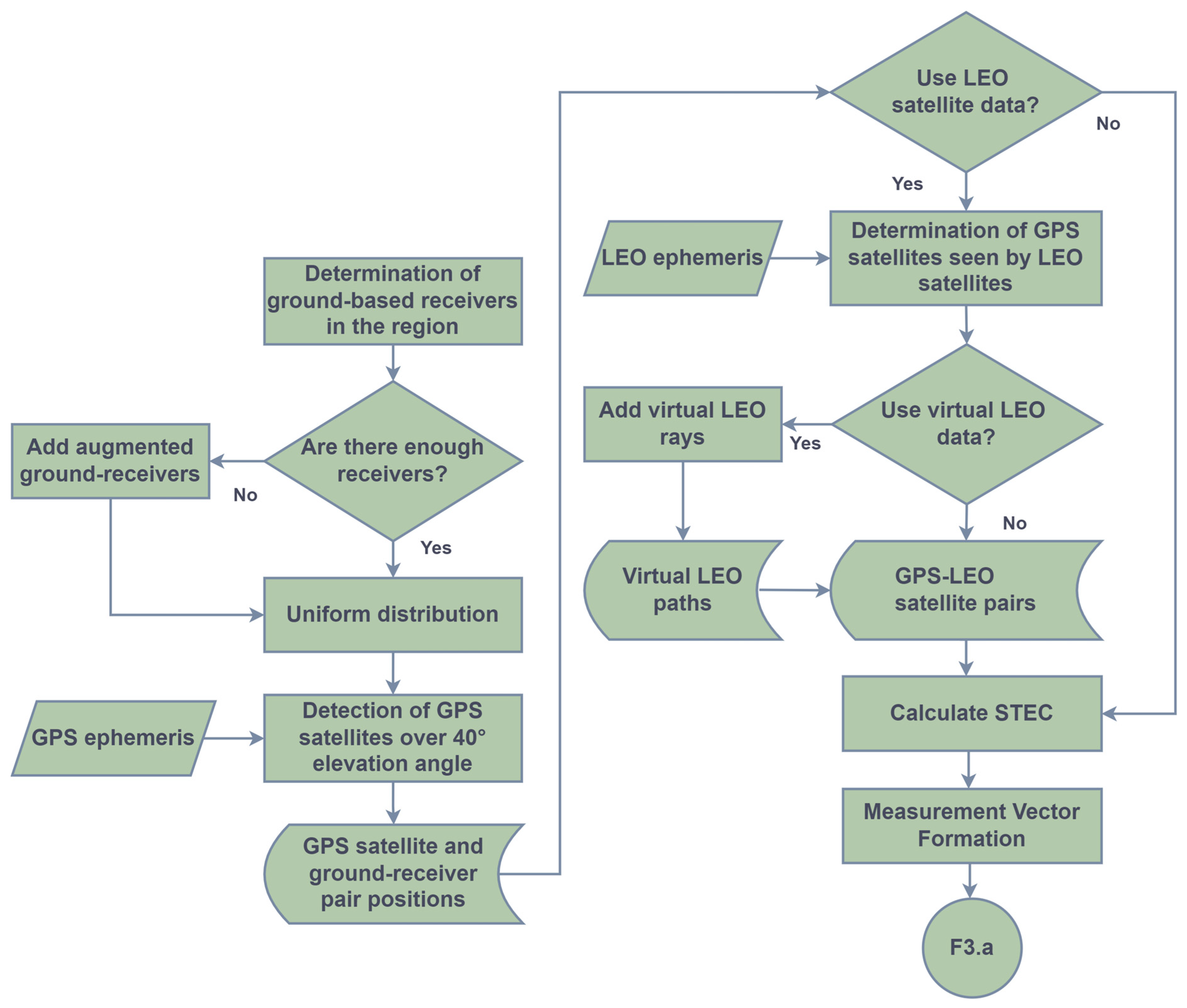
In the densely populated ground-based receiver region of Europe, we conducted a study to prevent overlapping rays between the receivers and GPS satellites within the same voxels, thus mitigating the risk of overfitting. This was achieved by selectively reducing the number of stations, ensuring a uniform distribution after decimation. In the IONOLAB-Fusion algorithm, ground-based receiver stations in the region of interest were detected automatically, and a homogenously distributed subset was identified with a rate of about 20% using uniform sampling. Consequently, for the example region of this study, 48 almost uniformly distributed ground-based receivers out of possible 163 GPS receivers were chosen, as presented in Figure 8 with red circles.

The GPS satellites visible to these receivers at elevation angles exceeding 40° are identified automatically. Figure 11 illustrates the rays between the ground-based receiver station and GPS satellite pairs for 8 April 2015 at 12:00 UT. In Figure 11a, 3-D representations of rays between pairs are provided. The selected region is indicated as the patch and the GPS satellites are identified by their Pseudorandom Noise (PRN) numbers. Figure 11b displays the projection of the 3-D representation onto a 2-D latitude and longitude plane. Figure 11c depicts a zoomed-in plot focused on the boundary of the extended region.

The COSMIC-1 mission, launched on 15 April 2006, stands as the world’s first multi-satellite occultation mission [62]. Comprising six identical satellites, each positioned at 72° and an altitude of 810 km, COSMIC-1 is equipped with advanced GPS radio occultation receivers onboard. In this study, the position of the LEO satellites from the COSMIC-1 mission was used. If the user opts to utilize the rays between the receivers onboard the LEO satellites, the GPS satellites within the line of sight of the LEO satellites are identified automatically.

In this study, the optimal temporal resolution between the LEO and GPS satellite pairs was obtained by considering the wide sense stationarity (WSS) period of the midlatitude ionosphere, whose details are given in [63,64,65,66]. WSS is the duration where the first and second moments of the experimental probability density function remain unchanged. In the studies of [64,65,66], the WSS period of the midlatitude ionosphere was determined to be 11 min. Within the WSS period, the temporal resolution is chosen by taking two conflicting constraints into consideration. It is desirable to take as many samples as possible within the WSS period, and, at the same time, the slanted ray paths should not cross the same voxels for the given spatial resolutions in the formation of 3-D spherical voxels. Thus, a temporal resolution of 30 s was selected to prevent voxel overlap, thus ensuring that the rays from different pairs traverse distinct voxels. At the same time, 22 samples can be obtained within 11 min WSS periods. In Figure 12a, an example of the 3-D representations of the rays between GPS and LEO satellites for 8 April 2015, at 12:00 UT, during a 11 min WSS period with 30 s temporal resolution is given. Figure 12b displays the projection of the 3-D representation onto a 2-D latitude and longitude plane. Figure 12c depicts a zoomed-in plot focused on the boundary of the extended region.

The STEC data between the receiver and GPS satellite pairs were calculated to form the measurement vector in Equation (19). In this study, the GPS-STEC values were estimated using the IONOLAB-STEC algorithm given in [5,6,51] with a 30 s time resolution. The receiver Differential Code Biases (DCBs) were estimated using the IONOLAB-BIAS algorithm provided in [67]. IONOLAB-STEC was conveniently accessible as an online space weather service via www.ionolab.org (accessed on 10 November 2023) [68].

The STEC between the LEO and GPS satellites was computed using the IRI-Plas-STEC algorithm [54]. Online computation of the IRI-Plas model is provided at www.ionolab.org (accessed on 13 November 2023) [69]. In the studies of [70,71], it is shown that, for ground-based receiver station and GPS satellite pairs, IRI-Plas-STEC values are very similar to IONOLAB-STEC values for quiet days in the midlatitude ionosphere.

The IONOLAB-Fusion algorithm allows the user to define virtual slanted ray paths that traverse the ionosphere in a horizontal direction, as outlined in Flowchart F3.a and Algorithm 3.a of Section 3. For the example scenario given in Figure 11 and Figure 12 on 8 April 2015 at 12:00 UT, the number of actual ground to GPS satellite IONOLAB-STEC ray paths was 172; the number of actual GPS-LEO IRI-Plas-STEC ray paths in a WSS period was 41; and the number of virtual augmentation ray paths was 25.

In this study, the paths of the rays between ground-based and LEO-based receivers and GPS satellites were traced as they traversed the ionosphere using the wave propagation algorithm IONOLAB-RAY to generate the sampling matrix in Equation (18). The IONOLAB-RAY algorithm uses the IRI-Plas model to obtain the physical parameters of the ionosphere, such as the electron density. The sampling matrix is formed by calculating the path lengths in the voxels for the pairs, as given in F3.b and Algorithm 4 of Section 3. If desired, the IONOLAB-RAY algorithm can automatically input Global Ionospheric Map (GIM)-TEC values to update the background IRI-Plas model to the current state of the ionosphere. The GIM-TEC maps with a temporal resolution of 2 h and a spatial resolution with 2.5° in latitude and 5° in longitude are automatically interpolated in the IONOLAB-RAY algorithm for the user-selected resolutions in terms of latitude, longitude, and time. In this study, the GIM-TEC maps were obtained from the Center for Orbit Determination in Europe (CODE) (ftp://cddis.gsfc.nasa.gov/pub/gps/products/ionex/ (accessed on 13 November 2023)).

As depicted in F4 and Algorithm 5 of Section 3, the measurement matrix was formed using the sampling matrix and subspace basis vectors. The association between the measurement vector and the measurement matrix was established using basis coefficients. The basis coefficient vector was estimated in the least squares sense, as shown in Equation (22). Ionospheric electron density reconstruction was estimated using the basis coefficient vector and signal subspace basis vectors for $N_l=\mathrm{55,800}$ voxels for each time epoch in a closed form. In Figure 13, we present slice representations of the electron density reconstructions within a selected region of the ionosphere for both quiet and disturbed days at different times, as displayed in the leftmost column. The middle column shows the electron densities that were calculated using the IRI-Plas model for the same dates and times. The rightmost column depicts the differences between the electron density reconstructions and the densities calculated from the IRI-Plas model. The reconstruction results utilized only the ground-based receivers in the IONOLAB-Fusion algorithm. As shown in Figure 13a,d, the electron density was reconstructed using Model Matrix ${\underset{¯}{\underset{¯}{\mathrm{G}}}}_1$ for the ionospheric disturbed day of 25 April 2013, 03:00 UT and the ionospheric quiet day of 17 April 2011, 08:00 UT, respectively. As shown in Figure 13g, Model Matrix ${\underset{¯}{\underset{¯}{\mathrm{G}}}}_2$ was formed using $N_d=$ 1 for the ionospheric quiet day of 8 April 2015, 18:00 UT. As shown in Figure 13j, Model Matrix ${\underset{¯}{\underset{¯}{\mathrm{G}}}}_2$ was formed using $N_d=$ 3 for the ionospheric disturbed day of 24 April 2012, 23:00 UT. The slice heights were selected between 100 km and 500 km with a resolution of 100 km.

In Figure 13a, the electron density is shown for 25 April 2013 at 03:00 UT. During night hours, the ionization levels were low. The highest electron density was observed at 300 km in the southeast part of the region, followed by 400 km in the southwest part of the region. Figure 13d displays the electron density for 17 April 2011 at 08:00 UT. As the sun rises, the ionosphere begins to ionize, leading to an increase in electron density. The eastern part of the region exhibits higher electron density values due to the sunrise. The highest electron density is seen at 300 km on the east side of the region, with the lower altitudes also starting to ionize. In Figure 13g, the electron density for 8 April 2015 at 18:00 UT is provided. Compared to 08:00 UT, the electron density at 18:00 UT remained higher due to the cumulative effect of the solar radiation throughout the day. The highest electron density was at 300 km, spreading across the region. In Figure 13j, the electron density is shown for 24 April 2012 at 23:00 UT. Since ionization depends on solar radiation, after sunset, the electron density decreases at all altitudes. As the sun sets in the West, electron density values are higher in the western part of the region. The higher electron density depicted in Figure 13a when compared to Figure 13j can be attributed to the presence of a storm during the early hours of the day. Since there was a disturbance in the early hours of 25 April 2013, the electron density of that day, as reconstructed in Figure 13a, captured the increase in the disturbance more accurately than the electron density calculated using the IRI-Plas model shown in Figure 13b, as indicated by the positive difference in Figure 13c. On quiet days, as depicted between Figure 13d,i, the electron densities captured by the IONOLAB-Fusion and IRI-Plas approaches showed the most significant differences at 300 and 400 km slices, which is where the peak electron density occurs, as given in Figure 13f,i. There was a depletion in the electron density on 24 April 2012 at 23:00 UT due to a negative disturbance, which was detected by IONOLAB-Fusion, and this resulted in a negative difference that is visible in Figure 13l.

To validate the results obtained using IONOLAB-Fusion, the electron density values at the location of the ionosondes were compared with the ionosonde vertical electron density profiles. The ionosondes used in this study, along with their respective locations, are detailed in

Table 1. Selected ionosonde locations in Europe.

Ionosonde	Name	Country	Geographical Coordinates		Geomagnetic Coordinates
			Latitude (°)	Longitude (°)	Latitude (°)	Longitude (°)
DB049	Dourbes	Belgium	50.10	4.60	51.10	88.92
EB040	Roquetes	Spain	40.80	0.50	42.77	81.53
JR055	Juliusruh	Germany	54.60	13.40	53.95	99.49
PQ052	Pruhonice	Czechia	50.00	14.60	49.32	98.60

.

The normalized metric distance was obtained by calculating the ratio of the metric distances between two vectors to the reference vector as

$$\mathrm{N}\mathrm{L}2\left(\mathrm{\%}\right)=\frac{{‖\underset{¯}{z_1}-\underset{¯}{z_2}‖}_2}{{‖\underset{¯}{z_1}‖}_2}\times 100,$$

(24)

where $\underset{¯}{z_1}$ and $\underset{¯}{z_2}$ are two vectors. Symmetric Kullback–Leibler Distance (SKLD) provides the entropical distance between two probability density functions and compares the formal similarity [72]. The SKLD is calculated as

$$\mathrm{S}\mathrm{K}\mathrm{L}\mathrm{D}={\sum }_{n_l=1}^{N_l}{z}_1^{\prime }\left[n_l\right]\ln \frac{z_1^{\prime }\left[n_l\right]}{z_2^{\prime }\left[n_l\right]}+{\sum }_{n_l=1}^{N_l}{z}_2^{\prime }\left[n_l\right]\ln \frac{z_2^{\prime }\left[n_l\right]}{z_1^{\prime }\left[n_l\right]},$$

(25)

where ${\underset{¯}{z}}^{\prime }$, the empirical probability density function, is defined as

$${\underset{¯}{z}}^{\prime }=\frac{1}{\sum _{n_l=1}^{N_l}z\left[n_l\right]}\underset{¯}{z}.$$

(26)

The height at which the ionization reaches its peak is denoted as hmF2, while the corresponding peak value is defined as NmF2 [48]. The height at which the Single-Layer Ionosphere Model (SLIM) assumes that the ionosphere is an infinitely thin layer is the Chapman height, which is considered to be at 428.8 km [50,51]. Since the ionosonde provides the reconstructed vertical electron density profile values up to 1000 km using the near vertical incidence sounding ionograms, comparisons were determined up to 1000 km. The examples of the electron density profiles at the ionosonde positions were calculated from the electron density reconstructions given in Figure 13, and they were then plotted alongside the vertical electron density profiles obtained from the ionosondes and the vertical electron density profiles calculated by the IRI-Plas model, as shown in Figure 14. In Figure 14, the following electron density profiles are given: the ionospheric disturbed day of 25 April 2013 at 03:00 UT at the position of DB049 in Figure 14a; the ionospheric quiet day of 17 April 2011 at 08:00 UT at the position of PQ052 in Figure 14b; the ionospheric quiet day of 8 April 2015 at 18:00 UT at the position of JR055 in Figure 14c; and the ionospheric disturbed day of 24 April 2012 at 23:00 UT at the position of EB040 in Figure 14d.

As shown in Figure 14, the electron density that was reconstructed with IONOLAB-Fusion using the IRI-Plas model aligned better with the ionosonde vertical profiles up to hmF2. However, at higher altitudes, which is known as the topside, differences in the underlying models between the IONOLAB-Fusion and ionosonde inversion algorithms led to discrepancies between the reconstructed electron density values and ionosonde vertical electron density profiles [73]. This was especially the case beyond the Chapman height, where notable disparities emerged between the ionosonde vertical electron profiles and the reconstructed electron density profiles that were constructed by IRI-Plas.

The performance of the electron density reconstruction by IONOLAB-Fusion was evaluated by comparing the reconstructed electron density values at the ionosonde positions with the vertical electron density profiles of the ionosondes, and this was achieved by employing the comparison methods on different heights. The comparison methods were separately applied to the hmF2, Chapman, and 1000 km heights. Additionally, to assess the improvement of the tomography results compared with the ionospheric model, the electron density calculated by the IRI-Plas model at the ionosonde positions was also compared with the ionosonde vertical electron density profiles as reference values. The comparison results of Figure 14 are given in

Table 2. Comparison results for the date, time, and ionosondes given in Figure 14.

Date	Ionosonde	Height	$\mathbf{N}\mathbf{L}2$	$\mathbf{S}\mathbf{K}\mathbf{L}\mathbf{D}$	${\mathbf{N}\mathbf{L}2}_{\mathbf{I}\mathbf{R}\mathbf{I}-\mathbf{P}\mathbf{l}\mathbf{a}\mathbf{s}}$	${\mathbf{S}\mathbf{K}\mathbf{L}\mathbf{D}}_{\mathbf{I}\mathbf{R}\mathbf{I}-\mathbf{P}\mathbf{l}\mathbf{a}\mathbf{s}}$
17 April 2011 08:00 UT (quiet day)	PQ052	hmf2	6.61	$1.48\times {10}^{-2}$	21.64	$1.47\times {10}^{-2}$
		Chapman	8.18	$2.74\times {10}^{-2}$	29.63	$2.39\times {10}^{-2}$
		1000 km	11.83	$30.01\times {10}^{-2}$	29.61	$29.63\times {10}^{-2}$
8 April 2015 18:00 UT (quiet day)	JR055	hmf2	7.22	$1.58\times {10}^{-2}$	35.12	$1.69\times {10}^{-2}$
		Chapman	25.01	$0.75\times {10}^{-2}$	30.26	$0.78\times {10}^{-2}$
		1000 km	45.71	$13.58\times {10}^{-2}$	41.38	$14.34\times {10}^{-2}$
25 April 2013 03:00 UT (disturbed day)	DB049	hmf2	32.51	$21.11\times {10}^{-2}$	33.95	$20.23\times {10}^{-2}$
		Chapman	47.85	$28.72\times {10}^{-2}$	73.23	$31.17\times {10}^{-2}$
		1000 km	56.61	$48.87\times {10}^{-2}$	83.60	$49.87\times {10}^{-2}$
24 April 2012 23:00 UT (disturbed day)	EB040	hmf2	46.85	$19.17\times {10}^{-2}$	82.91	$13.16\times {10}^{-2}$
		Chapman	39.20	$19.81\times {10}^{-2}$	69.64	$13.54\times {10}^{-2}$
		1000 km	33.42	$22.10\times {10}^{-2}$	62.09	$18.08\times {10}^{-2}$

.

On the ionospheric quiet day of 17 April 2011 at 08:00 UT, at PQ052, the Model Matrix ${\underset{¯}{\underset{¯}{\mathrm{G}}}}_1$ was utilized and the electron density was reconstructed using IONOLAB-Fusion. It was observed that the reconstructed electron density closely resembled the vertical electron density of the PQ052 across all altitudes when compared to the IRI-Plas model. The similarity in SKLD values between the electron density reconstructed by IONOLAB-Fusion and the electron density calculated by the IRI-Plas model suggests that both models exhibited a similar shape to the vertical electron density of the PQ052 up to the Chapman height. However, both profiles differed from the vertical electron density profiles of the ionosonde after the Chapman height. Despite this, at 1000 km, the reconstructed electron density outperformed the one calculated by the IRI-Plas model. On the quiet day of 8 April 2015, at 18:00 UT, the model matrix ${\underset{¯}{\underset{¯}{\mathrm{G}}}}_2$ is formed by using $N_d=$ 1. Similarly, the reconstructed electron density at the hmF2 and Chapman heights closely matched the vertical electron density profile of the JR055 when compared to the electron density calculated by the IRI-Plas model. However, due to the model matrix only containing a priori information from the previous day, the reconstructed electron density was unable to accurately track the ionosonde vertical profile after hmF2. On the disturbed day of 25 April 2013 at 03:00 UT, Model Matrix ${\underset{¯}{\underset{¯}{\mathrm{G}}}}_1$ was utilized at DB049. The reconstructed electron density profiles exhibited a closer resemblance to the DB049 vertical electron profile in both value and shape compared to the electron density calculated by the IRI-Plas model at all altitudes, as indicated by the results with smaller values obtained from both the metric distance and SKLD methods. On the day of 24 April 2012 at 23:00 UT, at EB040, the ionosonde vertical electron density values utilized for normalization were relatively smaller compared to those depicted in Figure 14a,b. Consequently, the minor changes had a more pronounced impact, leading to larger metric distances. Moreover, the inability of the ionospheric models to precisely depict the ionosphere during disturbed days resulted in larger disparities in comparison to the method results for electron density profiles derived from both the IONOLAB-Fusion method and the IRI-Plas model. On the disturbed day of 24 April 2012 at 23:00 UT, Model Matrix ${\underset{¯}{\underset{¯}{\mathrm{G}}}}_2$ was formed using $N_d=$ 3. The reconstructed electron density profile better reflected the peak electron density value, NmF2, compared to the IRI-Plas model. However, due to the disturbance, the prior information in the model matrix could not accurately represent the current ionosphere. Consequently, the normalized metric distance and SKLD values were higher at this time. While the reconstructed electron density yielded better results in terms of metric distance, the SKLD values were larger due to the shift in the hmF2 height.

To calculate the overall results, Model Matrix ${\underset{¯}{\underset{¯}{\mathrm{G}}}}_1$ was formed using $N_d=90$ days for the MSA years for April, while ${\underset{¯}{\underset{¯}{\mathrm{G}}}}_2$ was formed using $N_d=$ 3 previous days for the specified dates and times. Electron density reconstruction was conducted by IONOLAB-Fusion utilizing both ${\underset{¯}{\underset{¯}{\mathrm{G}}}}_1$ and ${\underset{¯}{\underset{¯}{\mathrm{G}}}}_2$ for all the specified dates and times. The reconstruction involves ground-based receiver station and GPS satellite pairs, as well as LEO-GPS satellite pairs and virtual LEO paths.

Table 3. Overall comparison results of the chosen scenarios.

Days	Scenario	Height	${\mathbf{N}\mathbf{L}2}_{{\mathbf{G}}_1}$	${\mathbf{S}\mathbf{K}\mathbf{L}\mathbf{D}}_{{\mathbf{G}}_1}$	${\mathbf{N}\mathbf{L}2}_{{\mathbf{G}}_2}$	${\mathbf{S}\mathbf{K}\mathbf{L}\mathbf{D}}_{{\mathbf{G}}_2}$	${\mathbf{N}\mathbf{L}2}_{\mathbf{I}\mathbf{R}\mathbf{I}-\mathbf{P}\mathbf{l}\mathbf{a}\mathbf{s}}$	${\mathbf{S}\mathbf{K}\mathbf{L}\mathbf{D}}_{\mathbf{I}\mathbf{R}\mathbf{I}-\mathbf{P}\mathbf{l}\mathbf{a}\mathbf{s}}$
Quiet	S1	hmf2	24.97	$9.04\times {10}^{-2}$	27.26	$13.67\times {10}^{-2}$	32.51	$6.92\times {10}^{-2}$
		Chapman	27.12	$14.89\times {10}^{-2}$	27.32	$14.91\times {10}^{-2}$	31.91	$11.81\times {10}^{-2}$
		1000 km	35.15	$41.12\times {10}^{-2}$	34.32	$37.76\times {10}^{-2}$	35.22	$37.25\times {10}^{-2}$
	S2	hmf2	24.95	$9.03\times {10}^{-2}$	27.12	$13.31\times {10}^{-2}$	32.51	$6.92\times {10}^{-2}$
		Chapman	27.10	$14.89\times {10}^{-2}$	27.23	$14.78\times {10}^{-2}$	31.91	$11.81\times {10}^{-2}$
		1000 km	35.14	$41.12\times {10}^{-2}$	34.27	$37.71\times {10}^{-2}$	35.22	$37.25\times {10}^{-2}$
	S3	hmf2	24.68	$8.97\times {10}^{-2}$	24.34	$10.75\times {10}^{-2}$	32.51	$6.92\times {10}^{-2}$
		Chapman	27.29	$14.96\times {10}^{-2}$	26.17	$13.66\times {10}^{-2}$	31.91	$11.81\times {10}^{-2}$
		1000 km	35.42	$41.33\times {10}^{-2}$	33.72	$37.33\times {10}^{-2}$	35.22	$37.25\times {10}^{-2}$
	S4	hmf2	23.89	$8.85\times {10}^{-2}$	23.80	$10.28\times {10}^{-2}$	32.51	$6.92\times {10}^{-2}$
		Chapman	27.14	$14.85\times {10}^{-2}$	25.78	$13.52\times {10}^{-2}$	31.91	$11.81\times {10}^{-2}$
		1000 km	35.73	$41.28\times {10}^{-2}$	34.13	$38.08\times {10}^{-2}$	35.22	$37.25\times {10}^{-2}$
Disturbed	S1	hmf2	35.01	$21.02\times {10}^{-2}$	41.55	$44.54\times {10}^{-2}$	51.74	$99.56\times {10}^{-2}$
		Chapman	47.85	$28.72\times {10}^{-2}$	51.87	$30.85\times {10}^{-2}$	55.60	$63.85\times {10}^{-2}$
		1000 km	56.61	$48.87\times {10}^{-2}$	59.50	$48.61\times {10}^{-2}$	65.55	$77.45\times {10}^{-2}$

presents a comprehensive comparison of the tomography results and all the ionosonde vertical electron density profiles, which encompass all the quiet and disturbed days across all hours. Furthermore, the electron density values computed from the IRI-Plas model were compared with the same dataset, and they were also used as a reference. To assess the impact of the horizontal paths, reconstructions were performed with and without them in various scenarios. The scenario column in Table 3 indicates the dataset utilized in the IONOLAB-Fusion method for electron density reconstruction. In Scenario 1 (S1), reconstruction was performed using paths between only the ground-based receiver stations and GPS satellite pairs. In Scenario 2 (S2), the horizontal ray paths between the LEO-GPS satellite pairs at the epoch of concern were added to the data from S1. In Scenario 3 (S3), the paths between the LEO-GPS satellite pairs within the WSS period were added to the data from S1. Finally, in Scenario 4 (S4), virtual LEO rays were added to the data from S3, which comprise both horizontal and slanted actual, virtual, and augmented ray paths.

In S1, upon analyzing the comparison results up to hmF2 for quiet days, it was evident that the reconstruction results that used ${\underset{¯}{\underset{¯}{\mathrm{G}}}}_1$ and ${\underset{¯}{\underset{¯}{\mathrm{G}}}}_2$ exhibited greater similarity with the vertical electron density profile of the ionosonde compared to the electron density values calculated from the IRI-Plas model. Moreover, reconstructions utilizing ${\underset{¯}{\underset{¯}{\mathrm{G}}}}_1$ as the model matrix outperformed those using ${\underset{¯}{\underset{¯}{\mathrm{G}}}}_2$ in terms of the normalized metric distance. Examination of the SKLD results revealed that the IRI-Plas model results exhibited a similar shape to the ionosonde vertical electron density values compared to the reconstruction results utilizing ${\underset{¯}{\underset{¯}{\mathrm{G}}}}_2$. This similarity arises from the IRI-Plas model’s consistent performance in the midlatitude region during quiet days. Conversely, the reconstruction results utilizing ${\underset{¯}{\underset{¯}{\mathrm{G}}}}_1$ yielded SKLD values closer to those of the IRI-Plas model. This can be attributed to the incorporation of more a priori information in the model matrix. The comparison results of ${\mathrm{N}\mathrm{L}2}_{\mathrm{I}\mathrm{R}\mathrm{I}-\mathrm{P}\mathrm{l}\mathrm{a}\mathrm{s}}$ and ${\mathrm{S}\mathrm{K}\mathrm{L}\mathrm{D}}_{\mathrm{I}\mathrm{R}\mathrm{I}-\mathrm{P}\mathrm{l}\mathrm{a}\mathrm{s}}$ were identical for the quiet days across all scenarios. In S2, there is a slight enhancement in the results of the ${\mathrm{L}2\mathrm{N}}_{{\mathrm{G}}_1}$, ${\mathrm{S}\mathrm{K}\mathrm{L}\mathrm{D}}_{{\mathrm{G}}_1}$, ${\mathrm{L}2\mathrm{N}}_{{\mathrm{G}}_2}$, and ${\mathrm{S}\mathrm{K}\mathrm{L}\mathrm{D}}_{{\mathrm{G}}_2}$up to the hmF2 height with the addition of momentary RO data; however, this improvement was not substantial. Furthermore, incorporating the RO data within the 11 min WSS period led to an enhancement in the comparison method results of ${\mathrm{L}2\mathrm{N}}_{{\mathrm{G}}_2}$ and ${\mathrm{S}\mathrm{K}\mathrm{L}\mathrm{D}}_{{\mathrm{G}}_2}$. While there were improvements in the ${\mathrm{L}2\mathrm{N}}_{{\mathrm{G}}_1}$ and ${\mathrm{S}\mathrm{K}\mathrm{L}\mathrm{D}}_{{\mathrm{G}}_1}$ results in the S3 scenario, which utilized virtual LEO rays, there were also improvements in ${\mathrm{L}2\mathrm{N}}_{{\mathrm{G}}_1}$, ${\mathrm{S}\mathrm{K}\mathrm{L}\mathrm{D}}_{{\mathrm{G}}_1}$, ${\mathrm{L}2\mathrm{N}}_{{\mathrm{G}}_2}$, and ${\mathrm{S}\mathrm{K}\mathrm{L}\mathrm{D}}_{{\mathrm{G}}_2}$up to the hmF2 height. When analyzing the comparison of results up to the Chapman height and 1000 km for quiet days, it was noted that the electron densities that were reconstructed utilizing ${\underset{¯}{\underset{¯}{\mathrm{G}}}}_1$ and ${\underset{¯}{\underset{¯}{\mathrm{G}}}}_2$ produced better results in metric distances up to the Chapman height across all scenarios. However, at 1000 km, larger comparison results were obtained, specifically ones that are similar the results obtained by IRI-Plas. This discrepancy arises from the increased disparities between the ionospheric model utilized by IONOLAB-Fusion for reconstruction and the ionosondes employed for the inversion algorithm. These results suggest that, on quiet days, employing Model Matrix ${\underset{¯}{\underset{¯}{\mathrm{G}}}}_1$ generates electron density profiles, even without the use of RO data. Moreover, without the use of RO data, Model Matrix ${\underset{¯}{\underset{¯}{\mathrm{G}}}}_1$, which integrates more prior information, outperformed the results obtained from ${\underset{¯}{\underset{¯}{\mathrm{G}}}}_2$. Additionally, the incorporation of the RO data obtained from within a WSS period and virtual LEO rays enhanced the metric distance results up to the Chapman height for the tomography using both ${\underset{¯}{\underset{¯}{\mathrm{G}}}}_1$ and ${\underset{¯}{\underset{¯}{\mathrm{G}}}}_2$, with more pronounced improvements being observed when utilizing ${\underset{¯}{\underset{¯}{\mathrm{G}}}}_2$. Upon analysis of the results for the disturbed days up to the hmF2 height, Chapman height, and 1000 km, it was evident that electron density reconstruction using both ${\underset{¯}{\underset{¯}{\mathrm{G}}}}_1$ and ${\underset{¯}{\underset{¯}{\mathrm{G}}}}_2$ outperforms the electron density calculated by the IRI-Plas model. In particular, the results obtained from Model Matrix ${\underset{¯}{\underset{¯}{\mathrm{G}}}}_1$, which integrates more prior information, exhibited a superior performance when compared to ${\underset{¯}{\underset{¯}{\mathrm{G}}}}_2$. Scenarios S2 and S3 were not considered as there was no LEO ray pass through the region on disturbed days.

The TEC values for all the latitude and longitude points within the region could be calculated by multiplying the electron density within each voxel by the corresponding increment of the voxel height and then summing these products over the entire height range. The routinely provided GIMs from the IGS are widely regarded as a dependable ionospheric product. In this study, the GIMs sourced from the Center for Orbit Determination in Europe (CODE) were employed to assess the quality of the ionospheric TEC calculated by IONOLAB-Fusion. Additionally, the TEC calculated from the IRI-Plas model was compared with GIM-TEC to serve as the reference value. The TEC was computed from the IONOLAB-Fusion electron density profiles using the IRI-Plas-STEC algorithm [68] for each grid point in latitude and longitude for the reconstruction height. In Figure 15, examples of the TEC maps from CODE-GIM, IONOLAB-Fusion-TEC, and IRI-Plas-TEC are presented for the ionospheric quiet day of 8 April 2015 at 08:00 UT. CODE-GIM is typically provided with resolutions of 2.5° in latitude and 5° in longitude, and it is interpolated to a 1° resolution in both the latitude and longitude of the reconstruction. The maps are provided for the extended region that encompassed the region of interest, as shown in Figure 8.

As shown in Figure 15, the TEC map derived by IONOLAB-Fusion exhibited closer similarity to the GIM-TEC results both in terms of value and the distribution of electron density when compared to the TEC map generated from the IRI-Plas model. The difference between the maps can be calculated using the root mean square error (RMSE) as

$$\mathrm{R}\mathrm{M}\mathrm{S}=\sqrt{\frac{1}{N_{\theta }{N}_{\varphi }}{\sum }_{n_{\theta }=1}^{N_{\theta }}{\sum }_{n_{\varphi }=1}^{N_{\varphi }}{\left(x\left(n_{\theta },n_{\varphi }\right)-\widehat{x}\left(n_{\theta },n_{\varphi }\right)\right)}^2},$$

(27)

where $x$ denotes the GIM-TEC and $\widehat{x}$ represents the calculated TEC maps.

The RMS values were computed for all quiet and disturbed days of reconstruction, through all hours, and for all the grid points between CODE-TEC and the maps calculated by the IONOLAB-Fusion and IRI-Plas models. The comparison results are given in

Table 4. RMS comparison of the CODE-TEC, IONOLAB-Fusion-TEC, and IRI-Plas-TEC results for all quiet and disturbed days through all hours in April. These results were computed for all the grid points in the extended region up to 2800 km in height.

	$\mathbf{R}\mathbf{M}\mathbf{S}$ (TECU)
Days	IONOLAB-Fusion-TEC Map	IRI-Plas-TEC Map
Quiet	1.69	4.46
Disturbed	1.80	5.70

. For the extended region in Figure 8, the $N_{\theta }$ and $N_{\varphi }$ values in Equation (27) were 25 and 36, respectively, making 900 grid points in total. For the height, electron density computed up to 2800 km was used in the IRI-Plas-TEC and IONOLAB-Fusion-TEC maps.

It was observed that, when the GIM-TEC was taken as the ground truth, the TEC maps calculated with IONOLAB-Fusion performed excellently compared to those obtained from the IRI-Plas model, with improvements of 37.89% for quiet days and 31.58% for disturbed days (even though the full ionospheric and plasmaspheric heights up to the GPS satellite were not used).

The IONOLAB-Fusion algorithm, with its ease in implementation, accuracy in comparison with ionosonde and GIM-TEC, and reliability and robustness in application to any region on Earth, provides a versatile means of estimation and a method through which to update electron density profiles for any ionospheric condition. It was observed that augmentation of virtual rays within the wide sense stationarity period of the ionosphere enhanced the accuracy of the reconstruction results when compared to ionosonde and GIM-TEC. The overall excellent performance is evidence that IONOLAB-Fusion is a strong candidate for an effective method to reconstruct electron density profiles for any date, time, region, and ionospheric state.

5. Conclusions

In this study, we developed a 4-D, computerized ionospheric tomography algorithm, namely IONOLAB-Fusion, which can automatically incorporate an optimized number of both ground and LEO satellite-based GPS receivers. The user-friendly algorithm only demands the border coordinates of the region of interest, the date and time of the reconstruction, and the number of days to be included into the model matrix. The optimization of model matrix is achieved through two distinct approaches: the user can choose the formation of a model matrix based on an ionospheric background model that is ordered with years of similar solar activity for the desired month of reconstruction; or, in the second choice, the model matrix can include a background ionospheric model for the last three days before the desired date. After the formation of a 4-D ionosphere model, which is represented in spherical voxels for the desired month and times of reconstruction, the model matrix was subjected to singular value decomposition to obtain the singular values that contained the highest energy in decreasing order. IONOLAB-Fusion automatically detects the highest energy singular values in its determination of signal subspaces and related coefficients; these are used to multiply the corresponding basis vectors, which are combined through least square sense optimization. The measurement vector in STEC is constructed using an optimum number of GPS receivers in the region of interest to ensure uniform square sampling as much as possible. It is also performed so as to avoid different ray paths passing, both in the horizontal and vertical directions, through the same or very close voxels. The actual path distances that rays travel in a voxel are computed and represented in the sampling matrix. For the horizontal paths, the wide sense stationarity period of the ionosphere is considered as the spatio-temporal augmentation of rays between the GPS and LEO satellites. IONOLAB-Fusion provides state-of-the-art ionospheric tomography in a closed form for any region on Earth utilizing an optimum number of sampling, both for vertical and horizontal paths.

IONOLAB-Fusion was applied to Europe with an optimum number of 48 ground receivers. The GPS to LEO satellite ray paths were automatically detected, and the number of ray paths were augmented either using virtual or actual paths within the wide sense stationarity period of the ionosphere. The performance of the algorithm was demonstrated by forming the model matrix using the hourly monthly median structure of the ionospheric background model for the moderately solar active years and the month of April. The algorithm was tested on both the quiet and disturbed days of the MSA years. The performance was based on a comparison of the ionosonde profiles for the chosen days and hours up to different heights, both in terms of shape and also the normalized metric distance. IONOLAB-Fusion performed outstandingly in the reconstruction of midlatitude ionospheric electron density profiles, both for quiet and disturbed days for all hours, ionospheric states, and ionosonde locations, and this was achieved using only either the most significant or the two most singular values in a closed form.

It was observed that the best agreement between the ionosonde and reconstructed profiles was obtained on quiet days, as well as in the areas up to the peak ionization height and Chapman height when using an optimum number of ground receivers corresponding to about a 20% uniform sampling. Certain individual comparisons achieved up to 6.62 in NL2 and 1.48$\times {10}^{-2}$ in SKLD, such as for PQ052 on the quiet day of 17 April 2011 at 08:00 UT, using only ground GPS receivers. Even on the disturbed days, such as 24 April 2012 at 23:00 UT at EB040, the fit of the reconstructed electron density to that of the ionosonde up to the peak ionization height was 43.5% better than the fit of the model to the ionosonde in terms of normalized metric distance.

When we consider the overall performance of the algorithm across both quiet and disturbed days, over all hours and ionosondes, and for all heights, the best results were obtained when we optimized the ground receivers to uniform square sampling with about a 20% sampling rate and the inclusion of augmented virtual and actual horizontal ray paths within the wide sense stationarity period of the ionosphere. We observed IONOLAB-Fusion profiles surpassing those of the IRI-Plas model by 26.51% for quiet days and 32.33% for disturbed days at the peak height, and they were also found to be in agreement with the ionosonde electron density profiles.

Additionally, the TEC map calculated by the IONOLAB-Fusion and IRI-Plas models were compared by the GIM-TEC for the quiet and disturbed days of the ionosphere throughout different hours of the day. It was observed that the RMS difference between the maps calculated by IONOLAB-Fusion and GIM-TEC was 1.69 TECU for quiet days and 1.80 TECU for disturbed days, thus surpassing the maps calculated using the IRI-Plas model by 37.89% and 31.58%, respectively.

When using IONOLAB-Fusion, the user can opt to choose to form the model matrix from the previous 3 days for the desired hours of reconstruction. This option provides similar results for quiet days and can be implemented in a sliding window to obtain an updated ionosphere for nowcasting or forecasting applications. Yet, since the effects of a geomagnetic storm may not have been included in the model matrix of the past three days, reconstructions by model matrix involving all the possible disturbances with a long-term representation, such as 90 days, would be in a better agreement with the overall ionosonde profiles.

IONOLAB-Fusion provides a state-of-the-art, user-friendly computerized ionospheric tomography algorithm that updates ionospheric electron density profiles, which are constructed using both actual and virtual augmented ray paths. The algorithm can be utilized in filtering, smoothing, updating, nowcasting, and forecasting applications with ease and versatility. The results of the algorithm were shown to be in excellent agreement with the ionosonde profiles and also with GIM-TEC. The algorithm is also reliable and robust so that it can be applied for any region and any ionospheric state. Additionally, post-reconstruction, the updated electron density profiles can be incorporated into the model matrix to further improve future reconstructions.

References

1. Zolesi, B.; Cander, L.R. Ionospheric Prediction and Forecasting; Springer: Berlin/Heidelberg, Germany, 2014. [Google Scholar]
2. Austen, J.R.; Franke, S.J.; Liu, C. Ionospheric imaging using computerized tomography. Radio Sci. 1988, 23, 299–307. [Google Scholar] [CrossRef]
3. Arikan, O.; Arikan, F.; Erol, C.B. 3-D Computerized ionospheric tomography with random field priors. In Mathematical Methods in Engineering; Springer: Dordrecht, The Netherlands, 2007; pp. 325–334. [Google Scholar]
4. Arikan, O.; Arikan, F.; Erol, C.B. Computerized ionospheric tomography with the IRI model. Adv. Space Res. 2007, 39, 859–866. [Google Scholar] [CrossRef]
5. Arikan, F.; Erol, C.B.; Arikan, O. Regularized estimation of vertical total electron content from Global Positioning System data. J. Geophys. Res. Space Phys. 2003, 108, 1469. [Google Scholar] [CrossRef]
6. Arikan, F.; Erol, C.B.; Arikan, O. Regularized estimation of vertical total electron content from GPS data for a desired time period. Radio Sci. 2004, 39, 1–10. [Google Scholar] [CrossRef]
7. Hernández-Pajares, M.; Juan, J.; Sanz, J.; Colombo, O.L. Application of ionospheric tomography to real-time GPS carrier-phase ambiguities resolution, at scales of 400–1000 km and with high geomagnetic activity. Geophys. Res. Lett. 2000, 27, 2009–2012. [Google Scholar] [CrossRef]
8. Kursinski, E.R.; Hajj, G.A.; Bertiger, W.I.; Leroy, S.S.; Meehan, T.K.; Romans, L.J.; Schofield, J.T.; McCleese, D.J.; Melbourne, W.G.; Thornton, C.L.; et al. Initial results of radio occultation observations of Earth’s atmosphere using the Global Positioning System. Science 1996, 271, 1107–1110. [Google Scholar] [CrossRef]
9. Reigber, C. CHAMP mission status and perspectives. Suppl. EOS Trans. AGU 2000, 81, F307. [Google Scholar]
10. Beyerle, G.; Schmidt, T.; Michalak, G.; Heise, S.; Wickert, J.; Reigber, C. GPS radio occultation with GRACE: Atmospheric profiling utilizing the zero difference technique. Geophys. Res. Lett. 2005, 32, L13806. [Google Scholar] [CrossRef]
11. Hajj, G.A.; Lee, L.C.; Pi, X.; Romans, L.J.; Schreiner, W.S.; Straus, P.R.; Wang, C. COSMIC GPS ionospheric sensing and space weather. Terr. Atmos. Ocean. Sci. 2000, 11, 235–272. [Google Scholar] [CrossRef]
12. Raymund, T.D.; Austen, J.R.; Franke, S.J.; Liu, C.H.; Klobuchar, J.A.; Stalker, J. Application of computerized tomography to the investigation of ionospheric structures. Radio Sci. 1990, 25, 771–789. [Google Scholar] [CrossRef]
13. Jin, S.; Li, D. 3-D ionospheric tomography from dense GNSS observations based on an improved two-step iterative algorithm. Adv. Space Res. 2018, 62, 809–820. [Google Scholar] [CrossRef]
14. Yavuz, E.; Arikan, F.; Arikan, O.; Erol, C.B. Algorithms and basis functions in tomographic reconstruction of ionospheric electron density. In Proceedings of the 2005 13th European Signal Processing Conference, Antalya, Türkiye, 4–8 September 2005. [Google Scholar]
15. Bust, G.S.; Mitchell, C.N. History, current state, and future directions of ionospheric imaging. Rev. Geophys. 2008, 46, RG1003. [Google Scholar] [CrossRef]
16. Zhai, C.; Lu, G.; Yao, Y.; Wang, W.; Zhang, S.; Liu, J.; Peng, W.; Kong, J.; Chen, J. 3-D tomographic reconstruction of SED plume during 17 March 2013 storm. J. Geophys. Res. Space Phys. 2020, 125, e2020JA028257. [Google Scholar] [CrossRef]
17. Lu, W.; Ma, G.; Wan, Q. A review of voxel-based computerized ionospheric tomography with GNSS ground receivers. Remote Sens. 2021, 13, 3432. [Google Scholar] [CrossRef]
18. Garcia, R.; Crespon, F. Radio tomography of the ionosphere: Analysis of an underdetermined, ill-posed inverse problem, and regional application. Radio Sci. 2008, 43, 1–13. [Google Scholar] [CrossRef]
19. Krankowski, A.; Zakharenkova, I.; Krypiak-Gregorczyk, A.; Shagimuratov, I.I.; Wielgosz, P. Ionospheric electron density observed by FORMOSAT-3/COSMIC over the European region and validated by ionosonde data. J. Geod. 2011, 85, 949–964. [Google Scholar] [CrossRef]
20. Prol, F.S.; Hoque, M.M. A tomographic method for the reconstruction of the plasmasphere based on COSMIC/FORMOSAT-3 data. IEEE J. Sel. Top. Appl. Earth Obs. Remote Sens. 2022, 15, 2197–2208. [Google Scholar] [CrossRef]
21. Prol, F.S.; Hoque, M.M.; Hernández-Pajares, M.; Yuan, L.; Olivares-Pulido, G.; Von Engeln, A.; Marquardt, C.; Notarpietro, R. Study of Ionospheric Bending Angle and Scintillation Profiles Derived by GNSS Radio-Occultation with MetOp-A Satellite. Remote Sens. 2023, 15, 1663. [Google Scholar] [CrossRef]
22. Jiang, C.; An, Q.; Wang, S.; Nie, W.; Zhu, H.; Liu, G. Accuracy assessment of the ionospheric total electron content derived from COSMIC-2 radio occultation based on multi-source data. Adv. Space Res. 2024, 10, 5157–5170. [Google Scholar] [CrossRef]
23. Hong, J.; Kim, Y.H.; Chung, J.-K.; Ssessanga, N.; Kwak, Y.-S. Tomography reconstruction of ionospheric electron density with empirical orthonormal functions using Korea GNSS network. J. Astron. Space Sci. 2017, 34, 7–17. [Google Scholar] [CrossRef]
24. Amerian, Y.; Voosoghi, B.; Ghaffari, A. Tomographic reconstruction of the ionospheric electron density in term of wavelets. J. Aerosp. Sci. Technol. 2010, 7, 19–29. [Google Scholar]
25. Mitchell, C.N.; Spencer, P.S.J. A three-dimensional time-dependent algorithm for ionospheric imaging using GPS. Ann. Geophys. 2003, 46, 687–696. [Google Scholar] [CrossRef]
26. Al-Franek, O.J.S. Ionospheric Imaging for Canadian Polar Regions. Doctoral Dissertation, University of Calgary, Calgary, AB, Canada, 2013. [Google Scholar]
27. Zeilhofer, C.; Schmidt, M.; Bilitza, D.; Shum, C. Regional 4-D modeling of the ionospheric electron density from satellite data and IRI. Adv. Space Res. 2009, 43, 1669–1675. [Google Scholar] [CrossRef]
28. Farzaneh, S.; Forootan, E. Reconstructing regional ionospheric electron density: A combined spherical Slepian function and empirical orthogonal function approach. Surv. Geophys. 2018, 39, 289–309. [Google Scholar] [CrossRef]
29. Tuna, H.; Arikan, O.; Arikan, F. Regional model-based computerized ionospheric tomography using GPS measurements: IONOLAB-CIT. Radio Sci. 2015, 50, 1062–1075. [Google Scholar] [CrossRef]
30. Tuna, H.; Arikan, O.; Arikan, F. Model based computerized ionospheric tomography in space and time. Adv. Space Res. 2018, 61, 2057–2073. [Google Scholar] [CrossRef]
31. Yildiz, S.K. Investigation of the planar midlatitude ionospheric trend under different levels of solar activity. Adv. Space Res. 2023, 71, 2252–2268. [Google Scholar] [CrossRef]
32. Brunton, S.L.; Kutz, J.N. Data-Driven Science and Engineering: Machine Learning, Dynamical Systems, and Control; Cambridge University Press: Cambridge, UK, 2022. [Google Scholar]
33. Erturk, O.; Arikan, O.; Arikan, F. Tomographic reconstruction of the ionospheric electron density as a function of space and time. Adv. Space Res. 2009, 43, 1702–1710. [Google Scholar] [CrossRef]
34. Erdem, E.; Arikan, F.; Deviren, M.N.; Cor, I. A model based ray tracing algorithm for anisotropic and inhomogeneous ionosphere with GIM-TEC assimilation. In Proceedings of the 2015 7th International Conference on Recent Advances in Space Technologies (RAST), Istanbul, Turkey, 16– 19 June 2015. [Google Scholar]
35. Erdem, E.; Arikan, F. IONOLAB-RAY: A wave propagation algorithm for anisotropic and inhomogeneous ionosphere. Turk. J. Electr. Eng. Comput. Sci. 2017, 25, 1712–1723. [Google Scholar] [CrossRef]
36. Erdem, E. Electromagnetic Wave Propagation Model and Simulation in Ionosphere. Doctoral Dissertation, Hacettepe University, Ankara, Türkiye, 2017. [Google Scholar]
37. Erdem, E.; Arikan, F. Communication Parameters Derived from IONOLAB-RAY Algorithm. In Proceedings of the 42nd COSPAR Scientific Assembly, Pasadena, CA, USA, 14–22 July 2018. [Google Scholar]
38. Ardic, F. 2-D Reconstruction of Total Electron Content Using Singular Value Decomposition. Master’s Thesis, Hacettepe University, Ankara, Türkiye, 2023. [Google Scholar]
39. Alken, P.; Thébault, E.; Beggan, C.D.; Amit, H.; Aubert, J.; Baerenzung, J.; Bondar, T.N.; Brown, W.J.; Califf, S.; Chambodut, A.; et al. International geomagnetic reference field: The thirteenth generation. Earth Planets Space 2021, 73, 49. [Google Scholar] [CrossRef]
40. Gulyaeva, T. Storm time behavior of topside scale height inferred from the ionosphere–plasmasphere model driven by the F2 layer peak and GPS-TEC observations. Adv. Space Res. 2011, 47, 913–920. [Google Scholar] [CrossRef]
41. Gulyaeva, T.; Arikan, F.; Stanislawska, I. Inter-hemispheric imaging of the ionosphere with the upgraded IRI-Plas model during the space weather storms. Earth Planets Space 2011, 63, 929–939. [Google Scholar] [CrossRef]
42. Gulyaeva, T. Empirical model of ionospheric storm effects on the F2 layer peak height associated with changes of peak electron density. J. Geophys. Res. Space Phys. 2012, 117, A02302. [Google Scholar] [CrossRef]
43. Gulyaeva, T.; Arikan, F.; Sezen, U. TEC Proxy Index of Solar Activity for the International Reference Ionosphere and its Extension to Plasmasphere IRI-Plas Model. Int. J. Sci. Eng. Appl. Sci. 2017, 3, 144–150. [Google Scholar]
44. Sezen, U.; Gulyaeva, T.L.; Arikan, F. Performance of solar proxy options of IRI-Plas model for equinox seasons. J. Geophys. Res. Space Phys. 2018, 123, 1441–1456. [Google Scholar] [CrossRef]
45. Gulyaeva, T.; Arikan, F.; Sezen, U.; Poustovalova, L. Eight proxy indices of solar activity for the International Reference Ionosphere and Plasmasphere model. J. Atmos. Sol.-Terr. Phys. 2018, 172, 122–128. [Google Scholar] [CrossRef]
46. Feltens, J. The international GPS service (IGS) ionosphere working group. Adv. Space Res. 2003, 31, 635–644. [Google Scholar] [CrossRef]
47. Sayin, I.; Arikan, F.; Arikan, O. Regional TEC mapping with random field priors and kriging. Radio Sci. 2008, 43, 1–14. [Google Scholar] [CrossRef]
48. Budden, K.G. The Propagation of Radio Waves: The Theory of Radio Waves of Low Power in the Ionosphere and Magnetosphere; Cambridge University Press: Cambridge, UK, 1988. [Google Scholar]
49. Bilitza, D. International reference ionosphere 2000. Radio Sci. 2001, 36, 261–275. [Google Scholar] [CrossRef]
50. Schaer, S. Mapping and Predicting the Earth’s Ionosphere Using the Global Positioning System. Doctoral Dissertation, University of Bern, Bern, Switzerland, 1999. [Google Scholar]
51. Nayir, H.; Arikan, F.; Arikan, O.; Erol, C.B. Total electron content estimation with Reg-Est. J. Geophys. Res. Space Phys. 2007, 112, A11313. [Google Scholar] [CrossRef]
52. Bilitza, D.; McKinnell, L.-A.; Reinisch, B.; Fuller-Rowell, T. The international reference ionosphere today and in the future. J. Geod. 2011, 85, 909–920. [Google Scholar] [CrossRef]
53. Arikan, F.; Sezen, U.; Gulyaeva, T.L. Comparison of IRI-2016 F2 layer model parameters with ionosonde measurements. J. Geophys. Res. Space Phys. 2019, 124, 8092–8109. [Google Scholar] [CrossRef]
54. Tuna, H.; Arikan, O.; Arikan, F.; Gulyaeva, T.L.; Sezen, U. Online user-friendly slant total electron content computation from IRI-Plas: IRI-Plas-STEC. Space Weather 2014, 12, 64–75. [Google Scholar] [CrossRef]
55. Liu, L.; Wan, W.; Chen, Y.; Le, H. Solar activity effects of the ionosphere: A brief review. Chin. Sci. Bull. 2011, 56, 1202–1211. [Google Scholar] [CrossRef]
56. Gulyaeva, T.; Arikan, F.; Bilitza, D. Mitigation of challenge of recalibration of sunspot numbers using proxies of solar activity for the ionospheric models. In Proceedings of the VarSITI-Variability of the Sun and Its Terrestrial Impact, Irkutsk, Russia, 10–15 July 2017. [Google Scholar]
57. Gordiyenko, G.; Maltseva, O.; Arikan, F.; Yakovets, A. An evaluation of the IRI-Plas-TEC for winter anomaly along the mid-latitude sector based on GIM-TEC and foF2 values. Adv. Space Res. 2019, 64, 2046–2063. [Google Scholar] [CrossRef]
58. Koroglu, O.; Arikan, F. Regional ionospheric trend statistics: IONOLAB-PDF. Turk. J. Electr. Eng. Comput. Sci. 2017, 25, 1773–1783. [Google Scholar] [CrossRef]
59. Arikan, F.; Koroglu, O. A methodology for estimation of hourly-monthly stochastic trend characteristics of midlatitude ionosphere. Radio Sci. 2020, 55, 1–15. [Google Scholar] [CrossRef]
60. Koroglu, O.; Arikan, F.; Deviren, M.N. Regional and seasonal parametric probability density function estimation for total electron content. In Proceedings of the 2014 22nd Signal Processing and Communications Applications Conference (SIU), Trabzon, Türkiye, 23–25 April 2014; pp. 915–918. [Google Scholar]
61. Yenen, S.; Gulyaeva, T.; Arikan, F.; Arikan, O. Association of ionospheric storms and substorms of Global Electron Content with proxy AE index. Adv. Space Res. 2015, 56, 1343–1353. [Google Scholar] [CrossRef]
62. Lei, J.; Syndergaard, S.; Burns, A.G.; Solomon, S.C.; Wang, W.; Zeng, Z.; Roble, R.G.; Wu, Q.; Kuo, Y.H.; Holt, J.M.; et al. Comparison of COSMIC ionospheric measurements with ground-based observations and model predictions: Preliminary results. J. Geophys. Res. Space Phys. 2007, 112, A07308. [Google Scholar] [CrossRef]
63. Sayin, I.; Arikan, F.; Akdogan, K. Optimum temporal update periods for regional ionosphere monitoring. Radio Sci. 2010, 45, 1–9. [Google Scholar] [CrossRef]
64. Arikan, F.; Koroglu, O.; Yenen, S.D. Wide Sense Stationarity Period of Slant and Vertical Total Electron Content in Determination of Temporal Correlation of Midlatitude Ionosphere. In Proceedings of the 42nd COSPAR Scientific Assembly, Pasadena, CA, USA, 14–22 July 2018. [Google Scholar]
65. Koroglu, O. Statistical Analysis of Total Electron Content Using TPGN and TPGN-Active Network. Master’s Thesis, Hacettepe University, Ankara, Türkiye, 2017. [Google Scholar]
66. Yenen, S.D. Estimation of Total Electron Content and Receiver Bias for a GPS Network. Master’s Thesis, Hacettepe University, Ankara, Türkiye, 2017. [Google Scholar]
67. Arikan, F.; Nayir, H.; Sezen, U.; Arikan, O. Estimation of single station interfrequency receiver bias using GPS-TEC. Radio Sci. 2008, 43, 1–13. [Google Scholar] [CrossRef]
68. Sezen, U.; Arikan, F.; Arikan, O.; Ugurlu, O.; Sadeghimorad, A. Online, automatic, near-real time estimation of GPS-TEC: IONOLAB-TEC. Space Weather 2013, 11, 297–305. [Google Scholar] [CrossRef]
69. Sezen, U.; Gulyaeva, T.; Arikan, F. Online computation of International Reference Ionosphere Extended to Plasmasphere (IRI-Plas) model for space weather. Geod. Geodyn. 2018, 9, 347–357. [Google Scholar] [CrossRef]
70. Arikan, F.; Shukurov, S.; Tuna, H.; Arikan, O.; Gulyaeva, T. Performance of GPS slant total electron content and IRI-Plas-STEC for days with ionospheric disturbance. Geod. Geodyn. 2016, 7, 1–10. [Google Scholar] [CrossRef]
71. Yenen, S.D.; Arikan, F.; Gulyaeva, T. Comparison of IRI-Plas STEC and IONOLAB-STEC over a midlatitude GPS network. In Proceedings of the 2019 9th International Conference on Recent Advances in Space Technologies (RAST), Istanbul, Türkiye, 11–14 June 2019. [Google Scholar]
72. Nielsen, F.; Nock, R. Sided and symmetrized Bregman centroids. IEEE Trans. Inf. Theory 2009, 55, 2882–2904. [Google Scholar] [CrossRef]
73. Gok, G.; Alp, Y.K.; Arikan, O.; Arikan, F. A Method for Automatic Scaling of Ionograms and Electron Density Reconstruction. IEEE Trans. Geosci. Remote Sens. 2022, 60, 1–11. [Google Scholar] [CrossRef]
Figure 1. Illustration of a 3-D spherical voxel model of IONOLAB-Fusion for epoch n t .
Atmosphere 15 00675 g001
Figure 2. Flowchart F1 showing the model matrix generation steps.
Atmosphere 15 00675 g002
Figure 3. Flowchart F2 showing the steps of application of SVD to the model matrix.
Atmosphere 15 00675 g003
Figure 4. Flowchart F3.a showing the steps of the formation of the measurement vector.
Atmosphere 15 00675 g004
Figure 5. Flowchart F3.b showing the steps of the formation of the sampling matrix.
Atmosphere 15 00675 g005
Figure 6. Illustration of the ionosphere over Europe using 3-D spherical voxels and rays connecting ground-based receiver stations () and augmented receivers (●) with GPS satellite pairs, as well as the receivers onboard LEO satellites and GPS satellite pairs.
Atmosphere 15 00675 g006
Figure 7. Flowchart F4 showing the steps of electron density reconstruction.
Atmosphere 15 00675 g007
Figure 8. The ground-based receiver stations (red circles ) and ionosondes (blue triangles Atmosphere 15 00675 i001) in the region. The dashed frame denotes the region of interest within the enlarged region.
Atmosphere 15 00675 g008
Figure 9. (a) The singular values and (b) normalized cumulative energy for G ¯ ¯ 1 , as formed by three MSA years and the days in the month of April for all hours of investigation.
Atmosphere 15 00675 g009
Figure 10. (a) The Kp, (b) Dst, and (c) AE indices at the selected dates. The day boundaries are given as vertical red dashed lines. The disturbance indicators are provided in horizontal black dash dotted lines.
Atmosphere 15 00675 g010
Figure 11. (a) Instantaneous 3-D representation of the rays between ground-based receiver stations and GPS satellites, (b) Projection of rays to the Earth, (c) the rays that lay in the expanded region for 8 April 2015, at 12:00 UT.
Atmosphere 15 00675 g011
Figure 12. (a) A 3-D representation of the rays between LEO and GPS satellites, (b) projection of the rays to the Earth, and (c) the rays that lay in the expanded region on 8 April 2015 at 12:00 UT within a WSS period.
Atmosphere 15 00675 g012
Figure 13. Slices of electron densities with a 100 km resolution for different dates and times: (a) reconstructed using IONOLAB-Fusion on 25 April 2013 at 03:00 UT (disturbed day); (b) calculated by IRI-Plas on 25 April 2013 at 03:00 UT; (c) the difference between the IONOLAB-Fusion and IRI-Plas results for 25 April 2013 at 03:00 UT; (d) reconstructed results using IONOLAB-Fusion on 17 April 2011 at 08:00 UT (quiet day); (e) calculated by IRI-Plas on 17 April 2011 at 08:00 UT; (f) the difference between the IONOLAB-Fusion and IRI-Plas results for 17 April 2011 at 08:00 UT; (g) reconstructed using IONOLAB-Fusion on 8 April 2015 at 18:00 UT (quiet day); (h) calculated by IRI-Plas on 8 April 2015 at 18:00 UT; (i) the difference between IONOLAB-Fusion and IRI-Plas for 8 April 2015 at 18:00 UT; (j) reconstructed using IONOLAB-Fusion on 24 April 2012 at 23:00 UT (disturbed day); (k) calculated by IRI-Plas on 24 April 2012 at 23:00 UT; and (l) the difference between IONOLAB-Fusion and IRI-Plas for 24 April 2012 at 23:00 UT.
Atmosphere 15 00675 g013aAtmosphere 15 00675 g013b
Figure 14. The reconstructed electron densities by IONOLAB-Fusion and the electron densities calculated by IRI-Plas at the locations of the ionosonde and ionosonde vertical electron density profiles: (a) 25 April 2015 at 03:00 UT (disturbed day), DB049; (b) 17 April 2011 08:00 UT (quiet day), PQ052; (c) 8 April 2015 at 18:00 UT (quiet day), JR055; and (d) 24 April 2012 23:00 UT (disturbed day), EB040.
Atmosphere 15 00675 g014
Figure 15. TEC maps for 8 April 2015 at 08:00 UT obtained from (a) CODE-TEC, (b) IONOLAB-Fusion-TEC, and (c) IRI-Plas-TEC.
Atmosphere 15 00675 g015