Machine Learning to Characterize Biogenic Isoprene Emissions and Atmospheric Formaldehyde with Their Environmental Drivers in the Marine Boundary Layer

Abstract

Oceanic biogenic emissions exert a significant impact on the atmospheric environment within the marine boundary layer (MBL). This study employs the extreme gradient boosting (XGBoost) machine learning method and clustering method combined with satellite observations and model simulations to discuss the effects of marine biogenic emissions on MBL formaldehyde (HCHO). The study reveals that HCHO columnar concentrations peaked in summer with 8.25 × 10¹⁵ molec/cm², but the sea–air exchange processes controlled under the wind and sea surface temperature (SST) made marine biogenic emissions represented by isoprene reach their highest levels in winter with 95.93 nmol/m²/day. Analysis was conducted separately for factors influencing marine biogenic emissions and affecting MBL HCHO. It was found that phytoplankton functional types (PFTs) and biological degradation had a significant impact on marine biogenic emissions, with ratio range of 0.07~15.87 and 1.02~5.42 respectively. Machine learning methods were employed to simulate the conversion process of marine biogenic emissions to HCHO in MBL. Based on the SHAP values of the learning model, the importance results indicate that the factors influencing MBL HCHO mainly included NO₂, as well as temperature (T) and relative humidity (RH). Specifically, the influence of NO₂ on atmospheric HCHO was 1.3 times that of T and 1.6 times that of RH. Wind speed affected HCHO by influencing both marine biogenic emission and the atmospheric physical conditions. Increased marine biogenic emissions in air masses heavily influenced by human activities can reduce HCHO levels to some extent. However, in areas less affected by human activities, marine biogenic emissions can lead to higher levels of HCHO pollution. This research explores the impact of marine biogenic emissions on the HCHO status of the MBL under different atmospheric chemical conditions, offering significant insights into understanding chemical processes in marine atmospheres.

1. Introduction

Formaldehyde (HCHO) is the most abundant carbonyl compound in the atmosphere [1,2], playing a crucial role as a precursor for HO_X and O₃, influencing atmospheric oxidizing capacity [3,4,5,6]. Its high reactivity makes it an intermediate in the oxidation of almost all volatile organic compounds (VOCs) [3] and contributes to its short atmospheric lifetime of only a few hours [7]. In addition to the HCHO emanating from secondary formation, HCHO also can be emitted directly [3]. Industrial activities, power generation, and ship emissions are significant sources of HCHO in the coastal marine atmosphere. The column concentration of HCHO reaches levels as high as 1 × 10¹⁶ molec/cm² in the vicinity of the Yangtze River Estuary [3].

The marine boundary layer (MBL) constitutes a stable atmospheric layer directly influenced by the ocean at its base, characterized by pronounced seasonal variations [8]. This layer experiences the most frequent interactions between the atmosphere and the ocean [8,9,10]. On one hand, the physical and chemical processes within the MBL directly affect the marine ecosystem. On the other hand, the atmospheric quality within the MBL is significantly influenced by oceanic emissions, potentially impacting the air quality in coastal regions [8,10,11]. In remote marine environments less impacted by human activities, the levels of in situ produced HCHO typically remain below 500 ppt [12]. Biogenic volatile organic compounds (BVOCs), such as isoprene emitted from marine sources, contribute significantly to HCHO production through photochemical oxidation [5,13,14], making marine biogenic emissions the predominant source of HCHO in remote marine regions [12,15,16,17,18]. Isoprene and its oxidation product HCHO can have a significant impact on the atmospheric environment of remote marine regions. They can increase the levels of HO_X in the upper troposphere by more than 2.5%, leading to an increase in O₃ concentration of approximately 2–5 ppbv [5,6].

Measurements of BVOCs such as isoprene in estuarine marine regions are notably sparse [6,19,20]. Research on isoprene in the marginal seas of China (MSC), including the Bohai Sea (BS), Yellow Sea (YS), and East China Sea (ECS), has been constrained to specific times or locations [21,22,23,24]. Consequently, constructing models to estimate isoprene emissions becomes a favorable approach. Estimations of marine biogenic isoprene emissions are categorized into two modeling approaches: bottom-up and top-down [6]. Top-down estimations typically involve constraining global-scale models with measured isoprene flux data or atmospheric concentrations to infer isoprene emission intensities [25,26,27]. Currently, most estimates of marine-derived isoprene emissions employ a bottom-up approach. This involves integrating laboratory-measured isoprene emission rates from phytoplankton with satellite-derived phytoplankton biomass to calculate marine isoprene flux [28,29,30]. Common methodologies include biogeochemical models and steady-state models for isoprene production. Biogeochemical models offer a more precise quantification of isoprene production and loss, along with the capability to couple with other oceanographic or meteorological models to describe isoprene’s transport in marine or atmospheric environments [31]. However, this necessitates more physical and chemical parameters of the ocean and atmosphere as input and demands higher computational resources during runtime [32]. Although the accuracy of steady-state production models for isoprene is relatively lower, they only require basic parameters such as chlorophyll-a and sea surface temperature to simulate isoprene production and emission quite accurately, leading to the prevalent use of steady-state models in simulating marine isoprene emissions [19,20,33,34,35].

Currently, there are two main methods for simulating atmospheric components: atmospheric numerical models and statistical prediction methods [36,37]. Numerical models predict and simulate pollutants based on atmospheric dynamics theory, employing a series of partial differential equations to simulate various physical and chemical processes of atmospheric pollutants [38]. Compared to atmospheric numerical models, statistical prediction algorithms are simpler, more efficient, and cost-effective. Initially, machine learning methods were often employed to rectify biases in simulations produced by models like Goddard Earth Observing System-Chem (GEOS-Chem) due to their outstanding learning performance [39,40]. With the development of artificial intelligence technology, machine learning methods within statistical prediction algorithms are increasingly gaining attention. The greatest advantage of machine learning lies in its capability to represent any type of nonlinear relationship between variables from different data sources [41], especially crucial for characterizing air pollutants, given the complex interactions among these variables [42]. Moreover, in the field of Earth system science, some newly developed machine learning models have outperformed traditional numerical models [41,43]. Random Forests (RF), Decision Tree Regression (DTR), and the eXtreme Gradient Boosting (XGBoost) algorithm, among others, have been widely utilized for simulating atmospheric components such as VOCs, NO_X, O₃, PM_2.5, and more [36,42,44,45,46,47]. The XGBoost method has become the most widely used machine learning approach in the field of atmospheric composition simulation due to its excellent learning performance on atmospheric components and strong interpretability [42].

Approximately 30% of the Chinese population resides in the coastal regions of the MSC area, making the atmospheric quality changes in the MSC region have a certain degree of impact on coastal residents [48]. Simultaneously, intensive human activities exert significant impacts on the marine environment and the MBL atmosphere above the MSC [49,50]. Therefore, this study focuses on elucidating the driving factors behind marine emissions and the MBL HCHO and exploring the influence of marine biogenic emissions transform to MBL HCHO under different atmospheric physical and chemical conditions. This study employed the XGBoost algorithm to develop machine learning models for marine biogenic emissions and MBL HCHO, coupling two XGBoost models to establish a comprehensive machine learning framework linking biogenic source elements and environmental factors to MBL HCHO. Using this framework in conjunction with air mass clustering algorithms, we discuss the roles of various environmental factors and marine biogenic emissions on MBL HCHO within different air mass types. This research lays the groundwork for a deeper investigation into the chemical characteristics of marine biogenic emissions within MBL, which enhances our understanding of the causes of marine atmospheric pollution.

2. Materials and Methods

2.1. Data Description and Preprocessing

This study utilized satellite observations of HCHO and NO₂ vertical column densities (VCDs), sea surface 10 m wind speed (U₁₀), 2 m surface temperature (T), relative humidity (RH), and downward surface solar radiation (SSRD) data to train the machine learning model for atmospheric HCHO. Chlorophyll-a (Chl-a) data from the surface layer of seawater, photosynthetically active radiation (PAR) data, sea surface temperature (SST) data, mixed-layer depth (MLD) data, and U₁₀ data were input into the steady-state model of isoprene for calculating the sea–air isoprene flux. These data were also used for training and validating the machine learning model for sea–air isoprene flux.

The level-2 HCHO and NO₂ data used in this study were sourced from the Tropospheric Monitoring Instrument (TROPOMI), which is part of the Sentinel-5P satellite launched by the European Space Agency (ESA) on 13 October 2017. The Sentinel-5P satellite is equipped with the TROPOMI [51], which provides global observations of trace gas components with a local time of 13:30 and a resolution of 7 km × 3.5 km [52]. For the analysis, the tropospheric vertical column densities (VCDs) of HCHO and NO₂ were derived from data with mass factors exceeding 0.5 and 0.75, respectively. Additionally, the pixel values for HCHO and NO₂ products were further resampled to a grid of 5 km × 5 km. For the HCHO data, an additional 25 km smoothing radius was applied to reduce noise in the data [3,4,53,54].

The chlorophyll-a (Chl-a) concentration and photosynthetically active radiation (PAR) data were obtained from the Himawari-9 satellite observations. Himawari-9 is the second satellite in the third-generation series of geostationary meteorological satellites operated by the Japan Meteorological Agency. Launched from the Tanegashima Space Center of Japan on 2 November 2016, Himawari-9 replaced Himawari-8 as the operational satellite on 13 December 2022 [55]. Operating at an altitude of approximately 35,800 km, the satellite’s subpoint is located at 140.7° E over the equator [56]. The Advanced Himawari Imager (AHI) aboard Himawari-9 has 16 spectral channels ranging from visible to infrared, enabling monitoring of the target area (from 60° N to 60° S, from 80° E to 160° W) with a high spatial resolution of 5 km and a high sampling frequency of 10 min [57,58].

The sea surface temperature (SST) and mixed-layer depth (MLD) data used in this study were sourced from the Hybrid Coordinate Ocean Model (HYCOM) reanalysis database. HYCOM provides data at a spatial resolution of 0.08° × 0.08° and a temporal resolution of three hours. The HYCOM database is a collection of ocean data based on output from the HYCOM model, encompassing spatial distribution and time series information of multiple ocean variables, including temperature profiles [59,60]. The HYCOM system employs the Navy Coupled Ocean Data Assimilation (NCODA) system to assimilate observational data, ensuring the accuracy and reliability of the data [61,62].

In order to maintain consistency in temporal resolution, the original sea temperature profile data obtained from the HYCOM database were interpolated using linear interpolation to generate gridded data in a 5 km × 5 km format. After interpolation, SST data were extracted by selecting the temperature of the water layer at 0 m depth from the ocean temperature profile data provided by the HYCOM system. The MLD was defined as the depth of the water layer where the temperature is 0.2 °C lower than the temperature at 10 m depth below the sea surface [63]. HYCOM provides temperature information for 41 vertical layers [64]. We employed a cubic spline interpolation method to interpolate temperature profiles of water layers, from which we derive the MLD data for the ocean.

This study utilized data from the European Centre for Medium-Range Weather Forecasts (ECMWF) Reanalysis version 5 (ERA5) database, including 10 m wind speed (U₁₀), 2 m surface temperature (T), dew point temperature (DT), and surface solar radiation downward (SSRD). Relative humidity (RH) was computed using T and DT [65]. ERA5 provides original gridded data with a spatial resolution of 0.25° × 0.25°. Linear interpolation was further employed to process ERA5 data into gridded data with a resolution of 5 km × 5 km.

2.2. Isoprene Production Model

The commonly used method to calculate the concentration and flux of isoprene in seawater is through the steady-state equilibrium between the production and loss processes of isoprene in seawater [19,34]. Models typically assume that isoprene is in a steady state composed of mass balance between biological production, chemical and biological losses, and emission to the atmosphere as Equation (1) [34].

$$P-LOSS-MIX=0$$

(1)

In Equation (1), “P” represents the total amount of isoprene produced by marine biological production that can be exchanged into the atmosphere. “LOSS” denotes the amount of isoprene chemically degraded and biodegraded in seawater. “MIX” represents the quantity of isoprene entering the atmosphere through sea–air exchange from seawater and the loss of isoprene to water mixing below the marine mixed layer.

Different phytoplankton functional types (PFTs) have distinct emission factors (EF, in $\mathsf{\mu }\mathrm{m}\mathrm{o}\mathrm{l}$ gchla⁻¹ day⁻¹) [66,67,68]. In this study, we utilized empirical relationships between surface Chl-a and PFT-specific diagnostic pigments to infer the composition of PFTs in water [69]. By combining this information with standardized isoprene production rates “P_chloro” observed in laboratory experiments, we calculated the total biological production of isoprene in the water [19,70]. Considering the influence of temperature and light on phytoplankton’s isoprene production process, we applied temperature and light corrections to the EF of phytoplankton [35,71,72,73], as shown in Equation (2).

$$p\left(h\right)=EF\cdot \frac{{\alpha }_1}{{\left(T+\delta \right)}^2+{\alpha }_2\cdot \left(T+\delta \right)+{\alpha }_3}\cdot l\mathrm{n}{\left(I\right)}^2$$

(2)

In Equation (2), p(h) represents the isoprene production rate of phytoplankton at depth h, the temperature correction coefficient $\delta$ and the light correction coefficient α are referenced from Zhang’s study [35,71], and I and T denotes the intensity of photosynthetically active radiation (in $\mathsf{\mu }\mathrm{E}$ m⁻² s⁻¹) and temperature (in °C) at depth h. Then, the production of isoprene in the water can be calculated using Equation (3) [71].

$$P=\frac{\beta }{MLD}\cdot \overline{\left[Ch{l}_a\right]}\cdot {\int }_0^{H}p\left(h\right) dh$$

(3)

The isoprene production of phytoplankton “P” can be obtained by integrating the isoprene production rate p(h) over the depth H, where H is the less of the MLD and the depth of the euphotic layer [35]. $\overline{\left[Ch{l}_a\right]}$ (in mg m⁻³) denotes the average column concentration of Chl-a, and its algorithm can be referenced from Zhang’s study [35,74]. β is a localized empirical coefficient, calculated based on the sampling data in the MSC region by Wu et al. [75], yielding β = 6.1558.

$$L_{bio}+L_{chem}=k_{bio}\cdot C_w+\left(\sum k_{chem,i}{C}_i\right)\cdot C_w$$

(4)

$$L_{mix}+L_{sea-air}=k_{mix}\cdot C_w+\frac{F_{sea-air}}{MLD}$$

(5)

$$F_{sea-air}=k_{AS}\cdot \left(C_w-\frac{C_A}{K_H}\right)=~k_{AS}\cdot C_w$$

(6)

During the degradation calculation, the model primarily considers biological degradation, chemical reaction, and mixing loss. Cw (water concentration of isoprene, in pmol L⁻¹) represents the concentration of isoprene in the water. Biological and chemical losses were set based on incubation experiment data [19,76], as shown in Equation (4), where k_bio was set to 0.14 ${\overline{\left[Ch{l}_a\right]}}^{1.28}$, and the chemical loss coefficient was set to 0.0527 day⁻¹. Mixing loss considers the processes of isoprene mixing into deeper layers and exchange with atmosphere, as shown in Equation (5), where k_mix was set to 0.005 day⁻¹ [31],. The loss through air–sea exchange was calculated based on the isoprene flux, as shown in Equation (6). Since the amount of isoprene in the atmosphere relative to the sea surface concentration is negligible [19,77], the sea–air isoprene flux (in nmol m⁻² day⁻¹) can be calculated using isoprene Cw, where k_AS can be obtained through empirical relationships with 10 m wind speed (U₁₀, in m s⁻¹) and sea surface temperature (SST, in °C) [20,34,78].

Substituting the production and loss of isoprene into Equation (1), the concentration of isoprene in seawater can be calculated as shown in Equation (7). Then, multiplying it by k_AS yields the sea–air isoprene flux.

$$C_w=\frac{P}{\left(\sum k_{chem,i}{C}_{Xi}+k_{bio}+\frac{k_{AS}}{MLD}+k_{mix}\right)}$$

(7)

2.3. Machine Learning Methods

This study employed the eXtreme Gradient Boosting (XGBoost) algorithm to simulate marine biogenic isoprene emissions and MBL HCHO VCDs. Chen and Guestrin developed XGBoost, utilizing a regularized gradient boosting algorithm to overcome overfitting issues [79]. Through iterative construction of multiple decision trees and their combination into a powerful model, the algorithm progressively improves model performance by optimizing the loss function at each step [42]. XGBoost starts with a simple model, typically a tree with only one leaf node, calculates the residuals for each sample, and then fits a new decision tree to reduce the residuals. The objective of this new decision tree is to capture a portion of the residuals. The process continues by adding the newly constructed tree to the model and iteratively building new decision trees to further reduce the residuals until reaching a predetermined number of trees or achieving an acceptable level of residuals. XGBoost introduces regularization terms to prevent overfitting and build reliable machine learning models like the sum of the squares of the leaf node weights [42,43,79,80,81].

During the learning process, the configuration of model hyperparameters significantly influences the accuracy of the results. Finding optimal hyperparameters is one of the most tedious tasks in machine learning. In this study, we utilized the Optuna framework for hyperparameter tuning. Optuna is a Python library for hyperparameter optimization, which employs Bayesian optimization and approximate target algorithms to efficiently and reliably identify the best hyperparameter configurations [82]. Specifically, this study trained XGB_Flux for calculating marine biogenic emissions (sea–air isoprene flux), and XGB_HCHO for estimating HCHO VCDs, with their respective hyperparameter configurations outlined in

Table 1. Hyperparameter configuration for training XGBoost models.

Model	n_Estimators	Learning_Rate	Max_Depth	Gamma	Subsample	Colsample_Bytree	Reg_Alpha	Reg_Lambda
XGBFlux	1900	0.086	5	0.21	0.97	0.81	0.14	0.52
XGBHCHO	1701	0.024	10	0.06	0.68	0.66	0.79	0.51

.

For model evaluation, common statistical metrics like the coefficient of determination (R²), root mean square error (RMSE), mean absolute error (MAE), and cross-validated coefficient of determination (CV-R²) were employed [83]. Cross-validation involves partitioning the dataset into k subsets, training the model on k-1 subsets, and validating it on the remaining subset. The average of the R² scores obtained from each validation is then calculated, resulting in the CV-R² score. CV-R² is a crucial metric for assessing the model’s generalization ability and robustness, providing a more reliable estimate of the model’s performance across different data subsets [84].

In addition, Shapley Additive exPlanations (SHAP) values were employed to interpret the trained machine learning models, which connects cooperative game theory with local explanations [85]. SHAP is a model-agnostic technique that can be applied to various machine learning methods, including the XGBoost method used in this study [40,79,85]. In the SHAP method, each input variable is considered a contributor to the outcome, and the contribution of each feature to the final prediction is measured by calculating the Shapley value of each input variable [85]. The aggregation of Shapley values from all sample points can assess the impact of input parameters on the target variable.

3. Results and Discussion

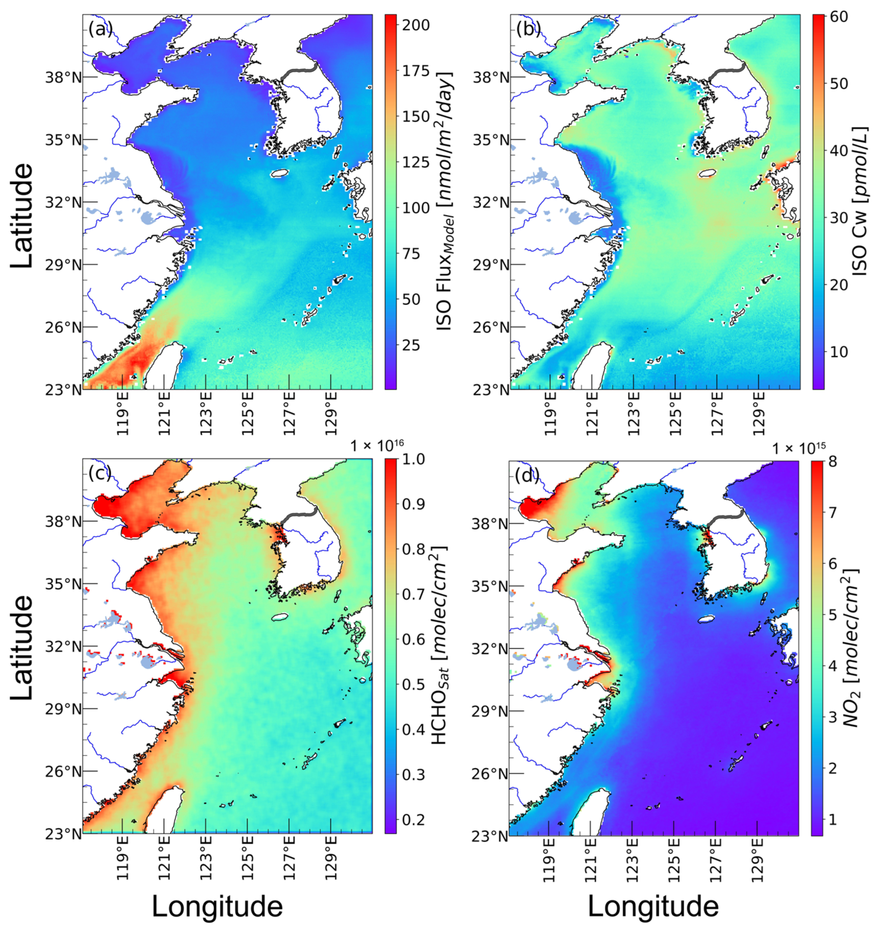
3.1. Spatiotemporal Distribution of Marine Biogenic Emissions and Trace Gas Components

Figure 1 illustrates the spatial distribution characteristics of sea–air isoprene flux (ISO Flux) and sea surface water concentration of isoprene (ISO Cw) from the production model, as well as the satellite-observed HCHO and NO₂ VCDs, over the marginal seas of China (MSC) region during the year 2023. The spatial distribution of the isoprene flux reveals that the average level in the coastal areas of northern China is only 31.03 nmol/m²/day. In contrast, the Taiwan Strait region exhibits a notably high isoprene flux reaching levels as high as 148.25 nmol/m²/day. Additionally, remote oceanic areas show relatively high levels reaching 60 nmol/m²/day, which is significantly higher than that in the northern coastal regions. These findings align well with historical survey results [24,75,86].

In the vicinity of the Korean Peninsula and Kyushu Island, isoprene Cw exhibits relatively high levels averaging about 35.42 pmol/L. The average isoprene Cw level in the Yellow Sea (YS) and East China Sea (ECS) regions is 29.13 pmol/L, while along the coast of Jiangsu Province, it is only 15.80 pmol/L, same as cruise survey results [21,24,75,87]. Despite the Taiwan Strait region showing higher isoprene flux levels, the average isoprene Cw level is only 23.17 pmol/L which is due to the influence of wind speed and sea temperature on the air-sea exchange process [20,34,78]. As illustrated in Figure S1c,e (in Supplementary Material), the SST and U₁₀ levels in the Taiwan Strait region are higher than those in the northern regions. Particularly in the Taiwan Strait, due to the effect of “Tip jet”, the wind speed is significantly higher compared to other regions, leading to intense air–sea substance exchange in this area and, consequently, higher isoprene flux levels but lower isoprene Cw levels compared to other areas [88,89].

HCHO is significantly impacted by human activities in coastal areas [3], exhibiting distinct high levels near the coast and lower levels further offshore. In the coastal regions of the Bohai Sea (BS), YS, and ECS, the average column concentration of HCHO reached as high as 9.23 × 10¹⁵ molec/cm², 8.90 × 10¹⁵ molec/cm², and 1.05 × 10¹⁶ molec/cm², respectively. In the more remote areas of the ECS and parts of the northwest Pacific Ocean, the average HCHO level was lower at 5.15 × 10¹⁵ molec/cm².

NO₂ displays a pronounced spatial distribution pattern, with high levels near coastal areas and lower levels in remote offshore regions, primarily due to anthropogenic emissions being the major source of NO₂ [7]. In remote marine areas with minimal human activity influence, the column concentration of NO₂ was relatively low at around 1.08 × 10¹⁵ molec/cm². However, significant high-value NO₂ areas appeared near the Bohai Bay, the coast of the Shandong Peninsula, and Shanghai, with average levels reaching 6.14 × 10¹⁵ molec/cm², attributed to shipping emissions in these regions. Given that NO₂ typically serves as an indicator of human activity intensity, the lower NO₂ levels and relatively higher HCHO levels in remote offshore regions suggest that besides direct emissions from human activities, a considerable portion of HCHO originates from secondary formation of marine source emissions such as isoprene in these areas [88,90,91].

Figure 2 illustrates the temporal variations of isoprene flux, Cw, atmospheric HCHO, and NO₂ VCDs in the MSC region in 2023. A comparison between Figure 2a,b reveals that the distribution characteristics of isoprene flux and Cw were entirely opposite. Isoprene flux exhibited a pattern of high values in autumn and winter and low values in spring and summer, with a relatively high peak in July. In contrast, isoprene Cw showed high values in spring and summer and low values in autumn and winter, with a relatively low point in July. The differences in the temporal variation characteristics between the two were controlled by factors influencing sea–air exchange of substances. Observation of Figure S2e reveals that U₁₀ exhibited a bimodal pattern under the influence of monsoons, with the main peak occurring in winter and a secondary peak in summer [89]. Therefore, in July, the intensity of material–air exchange was high, leading to significant loss of isoprene in seawater. As a result, July exhibited relatively high isoprene flux and relatively low Cw characteristics.

The temporal variations of HCHO VCDs exhibited a distinct feature of high levels in summer and low levels in winter, with the highest concentration level reaching 2.03 × 10¹⁶ molec/cm² in the BS region in July. Figure 2c reveals that the dispersion of HCHO in July was relatively higher compared to other months, with more grid below the 25th percentile density compared to June and August. This could be attributed to the higher U₁₀ in July, as oceanic winds influence the diffusion and transport processes of HCHO. In contrast, the temporal distribution pattern of NO₂ was opposite to that of HCHO, showing a characteristic of high levels in winter and low levels in summer. Since most areas of the MSC region are less affected by human activities, the background level of NO₂ was relatively low, resulting in less distinct temporal variations in NO₂ concentration. The highest level of NO₂ column concentration, reaching 2.34 × 10¹⁶ molec/cm², occurred near the mouth of the Yangtze River in December.

3.2. Construction of ML Model and Analysis of Influencing Factor

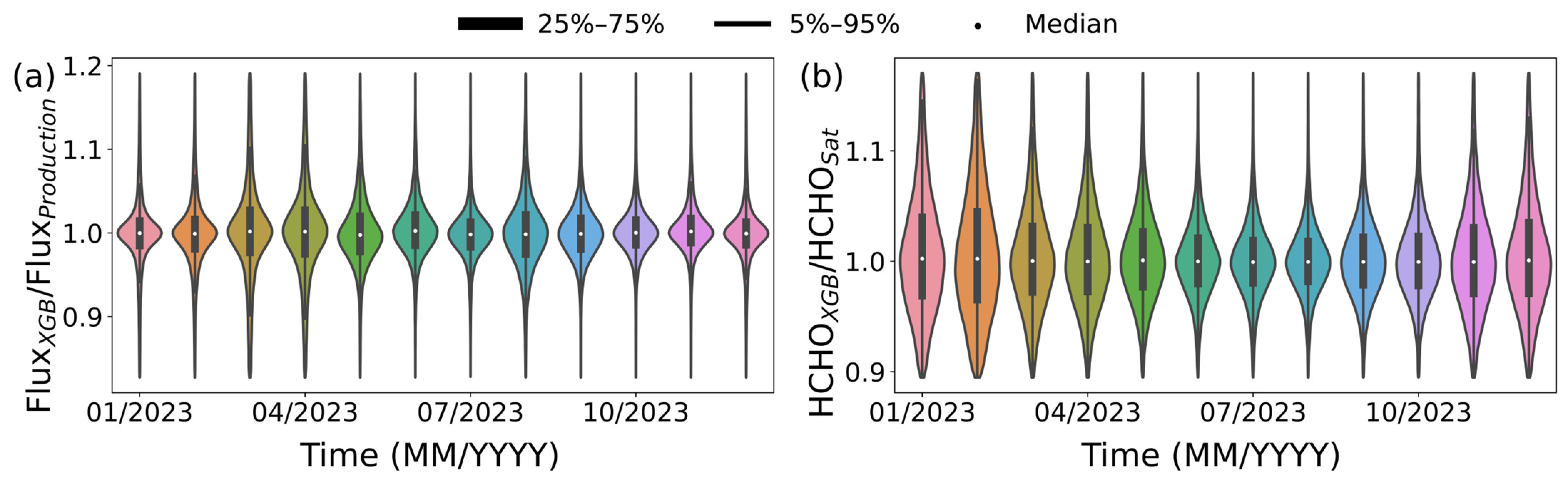
3.2.1. Construction of ML Model for Isoprene Flux and HCHO

This study employed the XGBoost algorithm to simulate the sea–air isoprene flux and atmospheric HCHO VCDs in the MSC region. When simulating flux, the model employed five parameters used in the marine isoprene production model: Chl-a, PAR, SST, MLD, and U₁₀. In the simulation of atmospheric HCHO VCDs, the model inputs included isoprene flux, NO₂, T, RH, SSRD, and U₁₀, where isoprene in the MSC region was considered as a reactant, with NO₂ serving as the chemical reaction atmospheric condition, and T, RH, SSRD, and U₁₀ were regarded as atmospheric physical conditions. The training process ensures that the data for each grid throughout the entire year of 2023 were involved in the training, thereby guaranteeing that the model learns the features of the target variable at different time points.

During the training of the XGBoost model, a total of 738,212 effective grid data were used, with 80% of this data used for model simulation and the remaining 147,643 data points reserved for model validation. The comparison between the model simulation results and the original data is illustrated in Figure S3, which shows the R² values between the simulated results of two models and the validation data were 0.9977 and 0.9756, respectively. The other three evaluation metrics also performed well, indicating that the simulated results can accurately reflect the characteristics of the original data.

To ensure the accuracy of XGBoost model learning results at spatiotemporal scales, the ratio of model-simulated results to input data was analyzed. The spatial distribution results are shown in Figure 3. Figure 3a displays the ratio between Flux_XGB obtained from the XGBoost model and Flux_Production calculated from the production model. It reveals an overestimation of Flux levels by the XGBoost model in the BS region, along the boundary between the Shandong Peninsula and the Jiangsu coast and in the central YS. Conversely, there was an underestimation of flux levels at the boundary between the YS and BS and along the Jiangsu coast. The spatial distribution of the ratio between simulated HCHO VCDs results and satellite observation data is depicted in Figure 3b as HCHO_XGB/HCHO_Sat. In the ECS and some areas of the northwestern Pacific Ocean, certain noise was observed, attributed to the background noise in the TROPOMI-observed HCHO data.

Figure 4a,b, respectively, depict the temporal evolution sequences of t_XGB/Flux_Production and HCHO_XGB/HCHO_Sat. Both exhibited no discernible temporal variations, indicating that the learning outcomes of XGBoost can capture the characteristics of isoprene flux and formaldehyde (HCHO) across different seasons. Their annual average levels were 1.00 ± 0.09 and 1.00 ± 0.03, respectively. In terms of isoprene flux, Flux_XGB/Flux_Production demonstrated its peak and nadir in February and December, with values of 1.08 ± 0.55 and 1.00 ± 0.08, respectively. As for HCHO VCDs, HCHO_XGB/HCHO_Sat reached its maximum and minimum values in February and October, at 1.01 ± 0.09 and 1.00 ± 0.05, respectively. The XGBoost model exhibited superior performance levels in winter compared to other seasons.

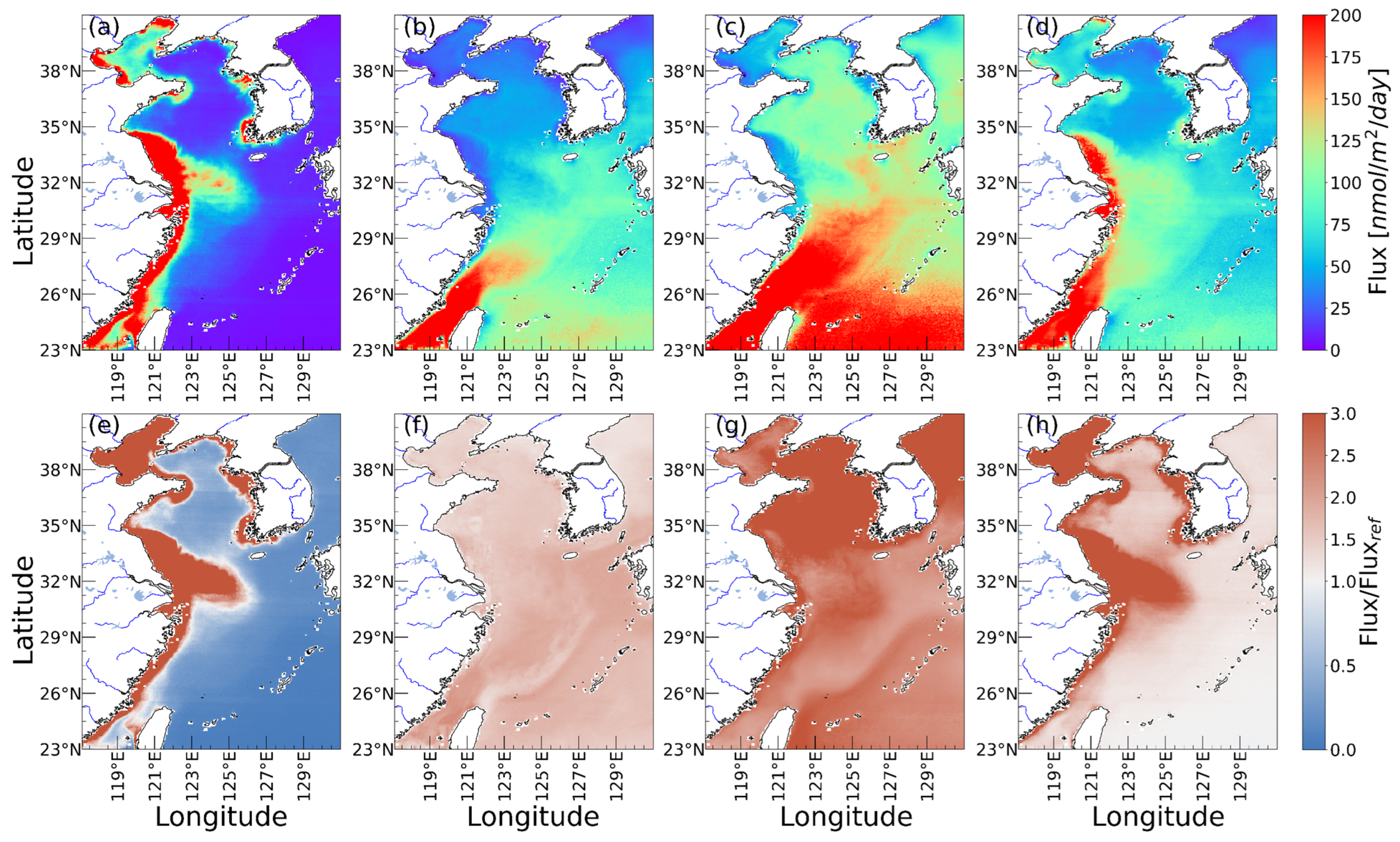
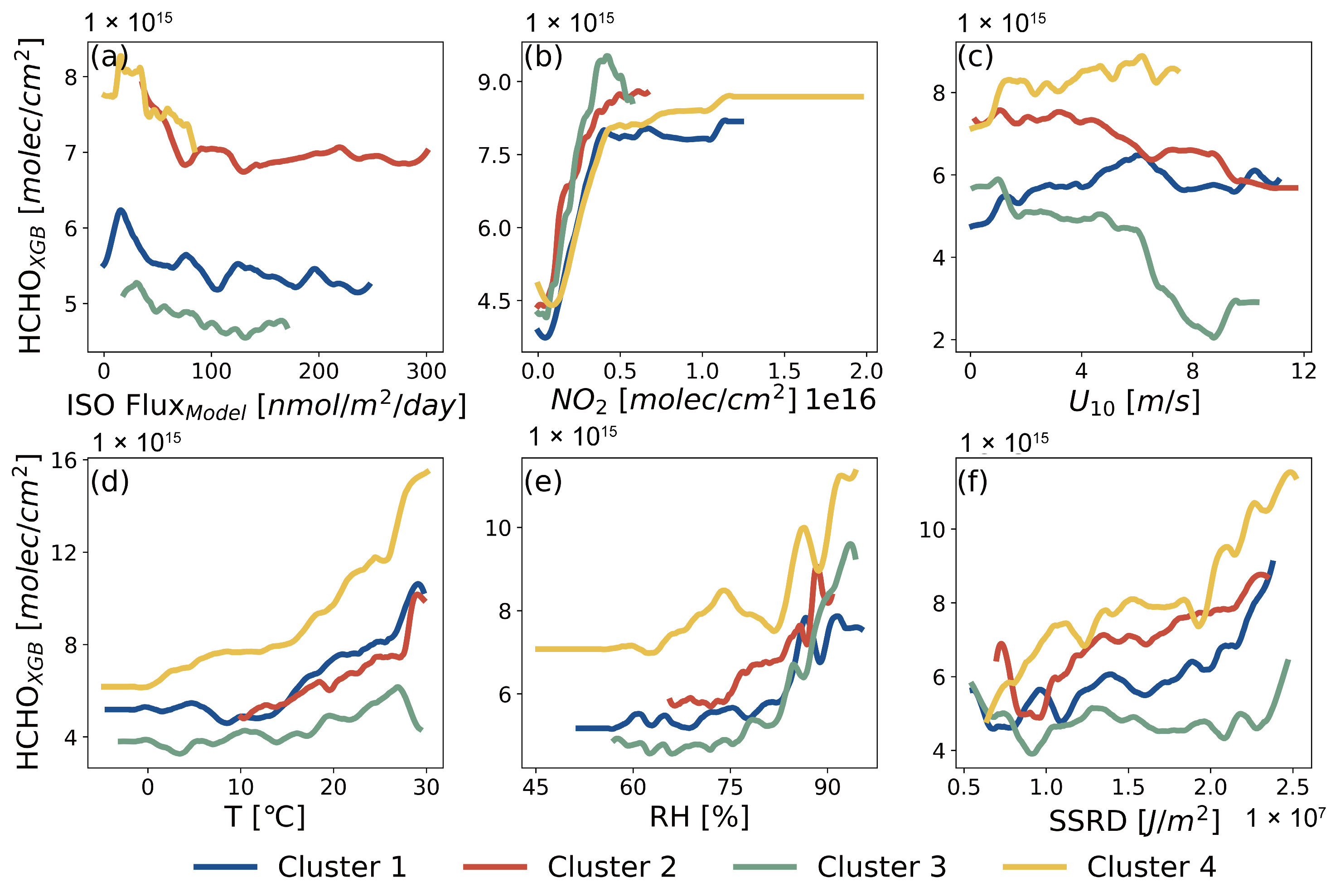
3.2.2. Assessment for Influencing Factors of Flux Based on Isoprene Production Model

Analyzing the factors influencing marine biogenic emissions and atmospheric HCHO is crucial for elucidating their relationship. This study utilized a marine isoprene production model to examine the impact of various factors on marine biogenic emissions. Four scenarios without considerations of phytoplankton functional types (PFTs), photosynthetically active radiation (PAR) attenuation in water, optimal temperature for phytoplankton isoprene production, and biodegradation based on phytoplankton abundance were evaluated. The calculated fluxes under these scenarios were compared with the fluxes used in this study (Flux_ref). The results are illustrated in Figure 5.

In the calculation of the noPFT scenario, the isoprene production model assumes that all phytoplankton functional types (PFTs) in seawater produce isoprene at the same rate, with the production rate being the mean value from laboratory cultivation experiments [19]. The computed results ”Flux_noPFT” are depicted in Figure 5a, where the high flux values were concentrated in coastal areas. In the coastal areas of the YS and ECS, the flux levels far exceed 200 nmol/m²/day, and the distribution of high-value areas perfectly aligns with the regions of high Chl-a concentrations as depicted in Figure S1a. Figure 5e illustrates the spatial distribution of Flux_noPFT/Flux_ref, revealing a significant overestimation of flux in areas with high Chl-a concentrations and a significant underestimation of flux in remote oceanic regions, with an average level of 15.87 ± 11.54 and 0.07 ± 0.04 respectively. This significant discrepancy indicates that the composition of PFTs exhibits considerable spatial variability, and the differentiation of PFTs can lead to substantial errors in the estimation of isoprene [31,67,92].

In the calculation of the noPAR scenario, it was assumed that there was no radiation attenuation in the water column. Compared to Equation (2), in this scenario, the photosynthetically active radiation (PAR) intensity at different depths was assumed to be the initial intensity I₀. Phytoplankton follow Equation (8) for the production of isoprene [31,35].

$$p\left(h\right)=EF\cdot \frac{{\alpha }_1}{{\left(T+\delta \right)}^2+{\alpha }_2\cdot \left(T+\delta \right)+{\alpha }_3}\cdot ln{\left(I_0\right)}^2$$

(8)

The computed results “Flux_noPAR” are depicted in Figure 5b, showing spatial distribution characteristics consistent with Flux_ref. Figure 5f illustrates that the spatial variability of Flux_noPAR/Flux_ref was minimal, with an average level of 1.32 ± 0.03, indicating a 30% overestimation of Flux when radiation attenuation is not considered [71].

In the calculation of the noT scenario, it was assumed that all phytoplankton were at their optimal temperature (OT) for isoprene production. In this case, the isoprene production rate by phytoplankton follows Equation (9) [31]. Compared to Equation (2), the temperature correction based on the OT has been removed. Instead, we only considered the impact of radiation attenuation of PAR in the water column on phytoplankton isoprene bioproduction.

$$p\left(h\right)=EF\cdot \frac{ln{\left(I\right)}^2}{ln{\left(I_0\right)}^2}$$

(9)

The computed results “Flux_noT” are depicted in Figure 5c, indicating that Flux_noT exhibited an overall higher level compared to Flux_ref. In the YS region, the isoprene flux level reached 93.19 ± 27.02 nmol/m²/day, while in the ECS region, the average flux level was 177.01 ± 59.63 nmol/m²/day. Figure 5g demonstrates that in the absence of consideration for OT, the level of Flux_noT/Flux_ref in the YS region can be as high as 2.75 ± 0.58, resulting in an overestimation of isoprene flux by approximately 275%. This is attributed to the presence of cold water masses in the YS, leading to relatively lower water temperatures and, consequently, less production of isoprene by phytoplankton. Conversely, the presence of the Kuroshio Current in the Taiwan Strait region brings its temperature closer to OT, resulting in a relatively smaller Flux_noT/Fluxref ratio between the Taiwan Strait and the ECS region. The biogeochemical model’s overestimation of isoprene in the Arctic [93] and Bering Strait [94] regions by more than twofold underscores the significant impact of optimal temperature on isoprene production from biological activity.

In the noK_bio scenario, the reference for K_bio was set at 0.005 day⁻¹ based on historical studies [19]. When considering the absence of biological degradation caused by phytoplankton abundance, as depicted in Figure 5d, the isoprene flux levels in all coastal areas and the ECS region were elevated compared to Flux_ref. Particularly noteworthy is the high flux level reaching 151.25 ± 80.06 nmol/m²/day along the Jiangsu coast. It becomes evident that the spatial distribution of Flux_noK_bio/Flux_ref closely resembles that of Flux_noPFT/Flux_ref in Figure 5h, exhibiting a similarity with the spatial distribution of Chl-a. The average level of Flux_noK_bio/Flux_ref in coastal areas was 5.42 ± 4.71. Due to the inherently lower Chl-a levels in remote oceanic regions, the level of biological degradation was lower, resulting in a ratio of 1.02 ± 0.03 in these regions. However, the abundance of organisms capable of degrading isoprene does not entirely correlate with Chl-a levels [95], indicating a need for further research on isoprene sinks [31].

Figure 6 illustrates the comparison between flux under four different scenarios and Fluxref, all of which result in an overestimation of isoprene flux. As depicted in Figure 6a, not considering PFTs led to an underestimation of flux when Chl-a levels were low. This could be attributed to high-yield populations dominating under low Chl-a levels. With increasing Chl-a levels, the degree of overestimation of flux gradually rose, consistent with the trend observed in Figure 6d. This suggests that higher Chl-a levels may correspond to relatively lower isoprene production but higher rates of biological degradation, indicating that Chl-a affects both the production and degradation of isoprene, resulting in a potentially non-monotonic effect on isoprene flux. In the noPAR and noT scenarios, lower levels of PAR and sea surface temperature (SST) corresponded to stronger overestimations of flux, indicating that higher PAR and SST levels favor the production and emission of isoprene.

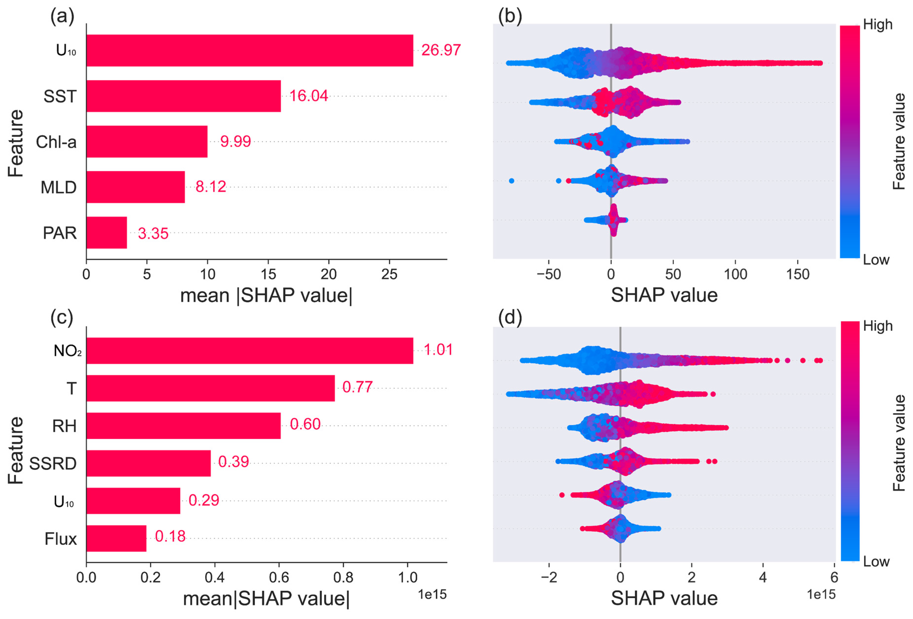
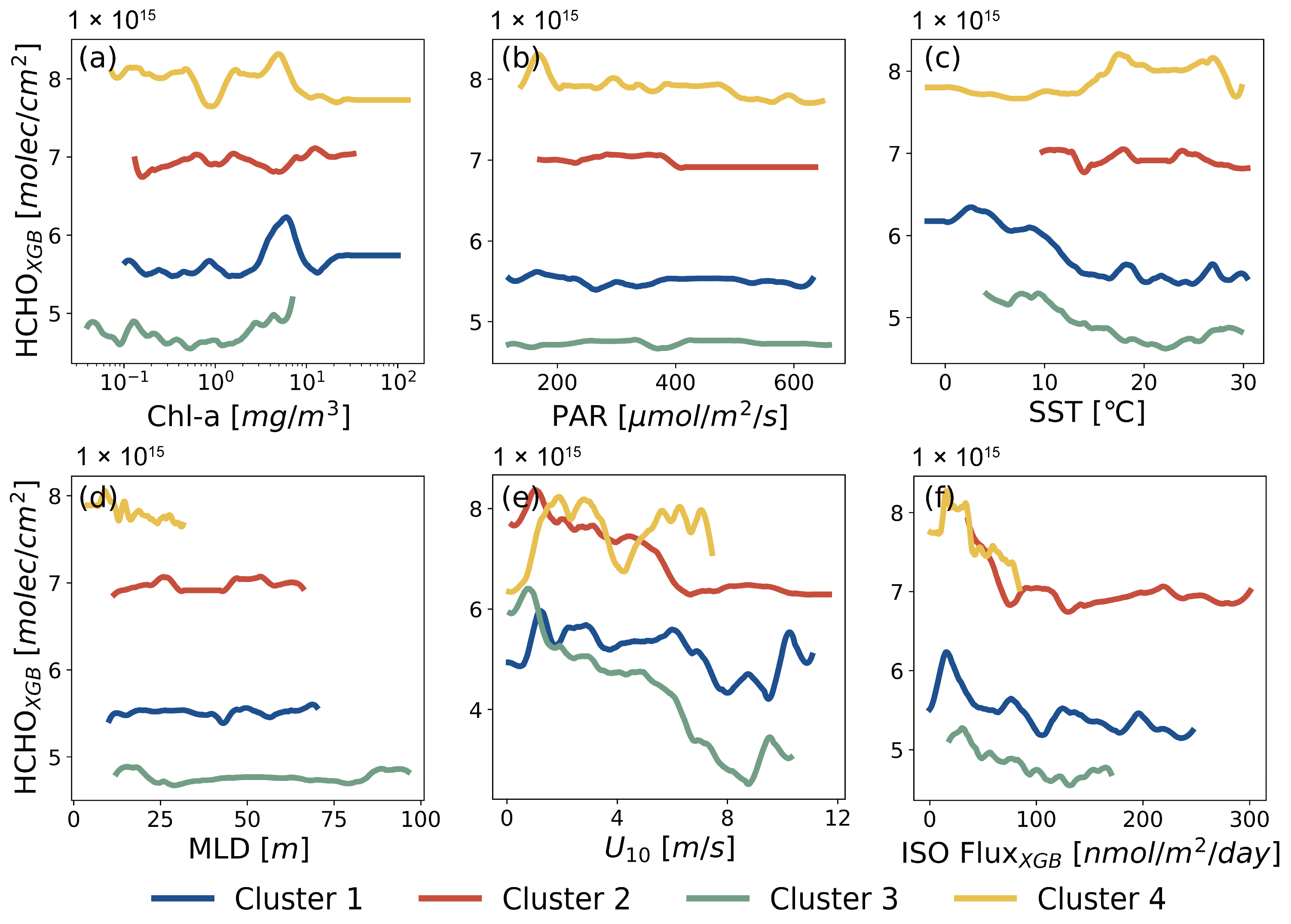
3.2.3. Assessment for Influencing Factors of Isoprene Flux and HCHO Based on XGBoost

Using the SHAP method, a quantitative analysis was conducted on the predictions of the two trained XGBoost models, followed by sorting the SHAP values of each parameter obtained; the results are presented in Figure 7. As illustrated in Figure 7a, the parameter with the greatest influence on isoprene flux is U₁₀, with an average SHAP value approximately eight times larger than that of the least important parameter, PAR. The next most influential parameters are SST and Chl-a. Among them, U₁₀ and SST are the primary factors controlling the exchange of isoprene between the ocean and the atmosphere. SST and Chl-a have a certain impact on the biological production of isoprene, indicating that the process of sea–air exchange has a greater impact on isoprene flux than the biological production of isoprene [32].

Figure 7b displays the SHAP values of each sample point. It can be observed that with an increase in U₁₀ levels, the SHAP value continuously increased, indicating that higher U₁₀ levels promote an increase in isoprene flux. The maximum SHAP value for SST occurred at moderate levels, suggesting a non-monotonic effect of SST on isoprene flux levels, indicating the existence of an optimal temperature for isoprene production and emission. For Chl-a, it was evident that higher Chl-a values corresponded to lower SHAP values of sample points, implying that excessively high Chl-a concentrations are detrimental to the production and emission of isoprene flux. This finding is consistent with the conclusions drawn from the analysis of factors based on the marine isoprene production model. It also demonstrates that the XGBoost model can capture the response of the target variable to changes in input parameters, enabling the use of the XGBoost model to analyze the impact of marine biogenic emissions on atmospheric HCHO [40,96].

Figure 7c illustrates the six parameters influencing HCHO levels. The parameter with the greatest impact on HCHO levels is NO₂, possibly because NO₂ can indicate the intensity of human activities. In areas heavily impacted by human activities, NO₂ and HCHO are typically directly emitted from anthropogenic sources, with anthropogenic HCHO accounting for over 90% of the total atmospheric HCHO [3,7,97]. Additionally, historical studies have suggested that NO_X can facilitate the conversion of atmospheric isoprene to HCHO [88,90,91]. Following NO₂ in importance are T and RH; as meteorological conditions, they can influence the conversion of isoprene and other BVOCs to HCHO and affect atmospheric chemical reactions involving HCHO.

Combining Figure 7d, it is evident that NO₂, T, RH, and SSRD all exhibited a positive correlation with HCHO levels, with higher parameter levels corresponding to larger SHAP values and stronger positive effects on HCHO levels. However, U₁₀ and isoprene flux demonstrated opposite characteristics. For U₁₀, it played a dual role in facilitating HCHO diffusion and promoting sea–air exchange processes. When U₁₀ levels were high, they primarily acted to dilute and disperse HCHO, resulting in negative SHAP values. Moreover, since high HCHO concentrations were mainly observed in regions influenced by human activities, higher isoprene flux levels may indicate lower levels of anthropogenic influence, leading to a situation where elevated isoprene flux levels correspond to decreased HCHO columnar concentrations.

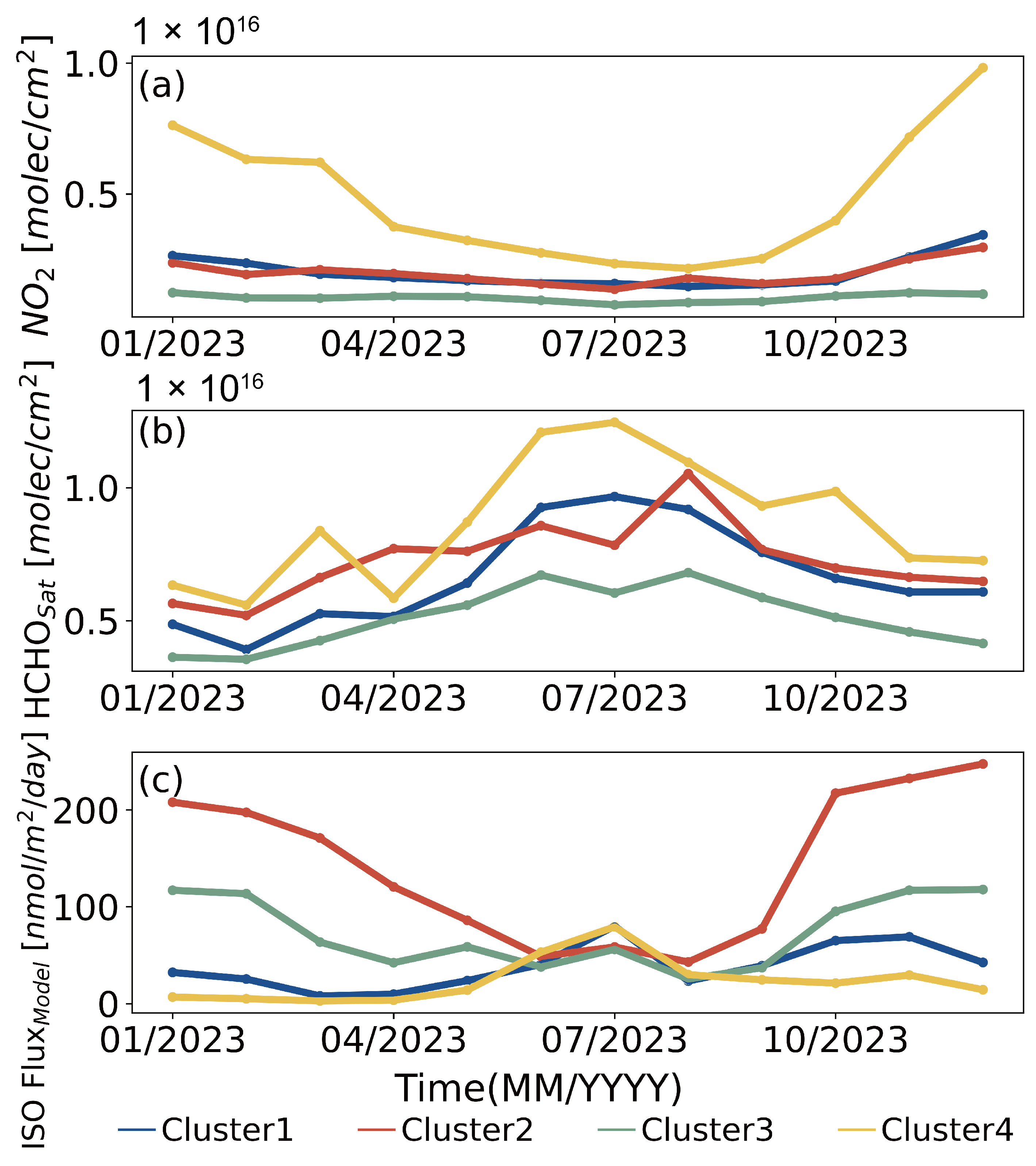
3.3. MBL HCHO under Different Air Masses Based on Clustering Methods

To further discuss the impact of marine biogenic emissions on the MBL HCHO under different environmental conditions, this study clustered air masses over the MSC region based on the levels of flux from isoprene production model and satellite-observed HCHO and NO₂ VCDs. Then, this study categorically discusses the influence of marine biogenic emissions on the MBL HCHO under different atmospheric chemical conditions.

3.3.1. Comprehensive Clustering of Air Masses and Characterization of Air Mass Parameters

The K-means method was utilized for air mass clustering. As depicted in Figure S4, the determination of the optimal number of clusters as 4 was based on the Silhouette Coefficient, Calinski–Harabasz Index, and Davies–Bouldin Index. Figure 8a illustrates the spatial distribution of the four air mass clusters. Figure 8b–d, along with

Table 2. The average levels of HCHO, NO₂, and ISO Flux in four air mass clusters.

Cluster	HCHO [molec/cm2]	NO2 [molec/cm2]	ISO Flux [nmol/m2/day]
Cluster 1	6.67 × 1015 ± 6.19 × 1014	2.03 × 1015 ± 6.18 × 1014	38.16 ± 12.95
Cluster 2	7.29 × 1015 ± 6.11 × 1014	1.97 × 1015 ± 3.25 × 1014	142.28 ± 27.64
Cluster 3	5.11 × 1015 ± 5.01 × 1014	1.04 × 1015 ± 2.09 × 1014	73.41 ± 15.51
Cluster 4	8.68 × 1015 ± 7.26 × 1014	4.83 × 1015 ± 1.21 × 1014	24.08 ± 7.34

, present the concentration levels of atmospheric components in the four air mass clusters. Cluster 1 primarily spanned over the YS and parts of the Sea of Japan. Cluster 2 was situated over the Taiwan Strait and its extension towards the ECS. Cluster 3 was distributed over the ECS and the northwestern Pacific region. Cluster 4 was predominantly found along the coastal areas from the BS, YS to Hangzhou Bay.

Clusters 1 and 2 were both situated in transition zones where human activity intensity decreased gradually, with similar levels of atmospheric pollutants. While Cluster 1 exhibiting slightly higher NO₂ concentration levels than Cluster 2, Cluster 2 stood out with the highest isoprene flux level among the four clusters, indicating a greater intensity of marine source emissions. Consequently, the concentration level of HCHO in Cluster 2 was higher than that in Cluster 1.

The region of Cluster 3 experienced minimal human activity influence, with its NO₂ level being approximately 50% of that in Cluster 1. However, its isoprene flux and HCHO levels were 192% and 76% of those in Cluster 1, respectively, indicating that marine source emissions are the primary source of atmospheric HCHO in remote oceanic regions. Cluster 4 was characterized by the strongest human activity influence, with its NO₂ and HCHO levels being 237% and 130% of those in Cluster 1, respectively. However, its isoprene flux level was only 63% of that in Cluster 1, suggesting that the primary source of HCHO in Cluster 4 air masses was from anthropogenic emissions.

Figure 9 illustrates the monthly variations in NO₂, HCHO, and isoprene flux levels among the four clusters. As depicted in Figure 9a, Cluster 4 exhibited the highest NO₂ levels, with a clear seasonal pattern of higher concentrations in winter and lower in summer. Clusters 1 and 2 showed similar NO₂ levels, with higher concentrations in winter and relatively stable levels throughout the remaining seasons. In contrast, Cluster 3, with minimal human activity influence, showed no significant fluctuations in NO₂ levels throughout 2023. Figure 9b displays the monthly variations in HCHO levels across the four clusters. All clusters demonstrated the characteristic pattern of higher concentrations in summer and lower in winter. However, in Cluster 2 and Cluster 3, characterized by higher marine source emissions, a relative trough in HCHO levels was observed in July, likely due to the high U₁₀ weather conditions during that month.

Similarly, as shown in Figure 9c, the isoprene flux levels in all clusters exhibited a relative peak with similar levels across clusters in July, attributed to the high U₁₀ conditions during that period. Cluster 2 and Cluster 3 showed a seasonal pattern of higher isoprene flux levels in winter and lower levels in summer. In contrast, Clusters 1 and 4, with lower isoprene flux levels, experienced peak levels in July. This aligns with the findings in Figure S5, where lower Chl-a levels in July coincided with a dominance of high-production phytoplankton, favoring the production of isoprene. Moreover, the temporal patterns of isoprene flux levels across clusters correspond to the variations in U₁₀ levels depicted in Figure S5e.

3.3.2. Impact of Isoprene on the MBL HCHO in Different Air Masses

The XGBoost model can effectively capture the response relationship between input parameters and the target variable [98,99]. Therefore, this study utilized the trained XGBoost model, XGB_HCHO, to investigate the relationship between marine biogenic emissions and the HCHO levels in the MBL. The study utilized the data ranges of the six input parameters used to simulate HCHO within different cluster air masses as parameter change intervals. These intervals were sequentially inputted into the XGB_HCHO model for simulation to analyze HCHO’s response within the range of each parameter. At this point, the remaining five parameters were set to the mean value of that parameter within the respective air mass cluster, and the results are depicted in Figure 10.

Figure 10a illustrates the response of HCHO to changes in isoprene flux from production model. Both Cluster 1 and Cluster 4 exhibited a noticeable decrease in HCHO VCDs as isoprene flux levels increased; this may be attributed to the higher degree of human activity influencing these two air mass clusters. An increase in isoprene flux levels signifies a reduction in human activity, leading to a shift in HCHO sources from anthropogenic to natural. Consequently, the HCHO VCDs decreased. In contrast, for Cluster 2 and Cluster 3 air masses, HCHO VCDs initially decreased and then increased with increasing isoprene flux levels; this is because when marine source emissions become the primary source of boundary layer HCHO, the enhancement of source emissions leads to an increase in HCHO levels [15,16].

Figure 10b demonstrates the response of HCHO to changes in NO₂ levels. It was observed that at low NO₂ levels, the HCHO VCDs in all air masses increased with increasing NO₂ levels. This is because NO₂ facilitates the conversion of BVOCs such as isoprene to HCHO. When NO₂ levels are high, the fluctuation in HCHO levels is reduced, as regions with high NO₂ levels have weaker biogenic emissions, resulting in a more stable HCHO concentration. Since NO₂ typically serves as an indicator of anthropogenic activity intensity, the level of correlation between NO₂ VCDs and HCHO VCDs can indirectly indicate the sources of HCHO in the atmosphere. As shown in Figure S6, a high level of $R_{HCHO-N{O}_2}^2$ was observed in the areas corresponding to Cluster 1 and Cluster 4. However, in most regions corresponding to Cluster 2 and Cluster 3, there was no significant correlation between the VCDs of HCHO and NO₂ in the atmosphere. Therefore, it can be inferred indirectly that in Cluster 2 and Cluster 3, most of the HCHO was not influenced by anthropogenic activities.

The response of HCHO to changes in U₁₀ levels is depicted in Figure 10c, where U₁₀ solely functions as a meteorological parameter influencing atmospheric component diffusion and transport. As indicated in Figure S5e, both Cluster 1 and Cluster 4 exhibited low wind speed levels. In these clusters, HCHO levels increased with rising U₁₀ levels, possibly due to the significant influence of human activities, as higher wind speeds facilitate the transport of HCHO from land to sea. On the other hand, Cluster 2 and Cluster 3 showed a rapid decrease in HCHO levels with increasing U₁₀ levels. This could be attributed to the swift dilution and dispersion of HCHO generated from marine biogenic emissions by oceanic winds. The response of HCHO to variations in T, RH, and SSRD across different clusters was consistent, as illustrated in Figure 10d–f. An increase in these meteorological parameters resulted in an elevation of HCHO levels, as it promoted the photochemical oxidation of VOCs into HCHO in the atmosphere.

As the temperature levels consistently rose, the levels of HCHO in Cluster 4 decreased. This suggests that the variability of meteorological conditions had a more pronounced effect on the levels of HCHO in Cluster 4, thus confirming that the mainly source of HCHO in Cluster 4 was from marine biogenic emissions. The response of HCHO levels to meteorological parameters in Cluster 2 and Cluster 3 was more consistent. However, the biogenic emission intensity in Cluster 2 was higher than in Cluster 3. Therefore, with the increase in RH and SSRD levels, the HCHO VCDs levels in Cluster 2 were stronger than those in Cluster 3. The differing response patterns of HCHO VCDs levels to parameter changes among different clusters indicate the distinct sources of HCHO in each cluster.

Furthermore, two XGBoost models was coupled to delve deeper into the relationship between marine biogenic emissions and the MBL HCHO levels. The output from XGB_Flux served as the isoprene flux input parameter for XGB_HCHO. This established a pathway from biogenic elements such as Chl-a and environmental factors to the MBL HCHO, facilitating the analysis of the effects of different biological elements and environmental factors influencing marine biogenic emissions on the MBL HCHO. It is noteworthy that the U₁₀ parameter in the coupled model was considered both as a meteorological parameter affecting the sea–air isoprene exchange and influencing the transport diffusion of HCHO. The response of HCHO to each parameter is depicted in Figure 11.

Firstly, focusing on Figure 11f, the response of HCHO levels to the variation in Flux_XGB of was consistent with Figure 10a. This arose arises because the assessment of HCHO’s response to the parameter influencing flux did not involve parameters other than the flux in XGB_HCHO. The impact of the four parameters other than U₁₀ on the MBL HCHO levels was relatively minor, especially for PAR and MLD. HCHO showed no significant response to changes in these two parameters across different clusters. Regarding Chl-a, as shown in Figure 11a, four clusters exhibited two response patterns. Clusters 1 and 4, corresponding to marine areas with a wide range of Chl-a variations, showed peak HCHO levels when Chl-a levels were around 6 mg/m³. HCHO levels fluctuated significantly within the range from 1 to 10 mg/m³, while the response of HCHO to Chl-a variations was less apparent at other concentration levels. Clusters 2 and 3 showed a decrease followed by an increase in HCHO levels with increasing Chl-a levels. The response of HCHO to variations in SST at the marine areas corresponding to the four clusters is illustrated in Figure 11c. When SST in these areas ranged from 20 to 25 °C, the response of HCHO was a decrease followed by an increase, suggesting the presence of SST conditions least favorable for marine biogenic emission affecting the MBL HCHO. HCHO’s response to changes in Chl-a and SST indicates the direct impact of biological activity intensity on HCHO levels. However, factors influencing biogenic emissions include not only those affecting biogenic activity but also U₁₀, which controls sea–air exchange processes.

Figure 11e illustrates the impact of U₁₀ in the coupled model on HCHO levels. Compared to Figure 10c, the response characteristics of HCHO to wind speed in the four clusters have changed to some extent. In conditions of low wind speed, compared to the scenario without considering the promotion of air–sea exchange by U₁₀, the levels of HCHO in Cluster 1 and Cluster 4 were lower, while those in Cluster 2 and Cluster 3 were higher. This suggests that at low wind speeds, maritime winds primarily facilitate air–sea exchange. As U₁₀ levels increased, HCHO levels in all four clusters showed a decreasing trend. When U₁₀ was around 4 m/s, HCHO levels decreased significantly in Cluster 4, while they decreased more gradually in the other three clusters. For Cluster 4, this indicates that maritime winds started to play a dilution role [3].

As U₁₀ levels rose to around 6 m/s, maritime winds began to transport HCHO from the surrounding environment to Cluster 4, leading to a rapid and steady increase in HCHO levels. At the same time, HCHO levels in the other three clusters also started to decrease sharply. However, with further increases in U₁₀ levels, HCHO levels in Cluster 1 started to rise again. This may have been because maritime winds transported HCHO from other areas to Cluster 1, but at this point, HCHO levels in Cluster 1 were lower than those in Figure 10c. HCHO levels in Cluster 2 remained stable, possibly because the high wind speeds in the Taiwan Strait region balanced the conversion of marine biogenic emissions to HCHO with the dilution effects of HCHO. In Cluster 3, HCHO levels started to rise when U₁₀ reached around 8 m/s, indicating that for remote ocean areas, higher wind speeds leading to higher marine biogenic emissions are the main reason for the increase in atmospheric HCHO levels. It is also evident that considering the influence of U₁₀ on isoprene flux, the HCHO levels in Cluster 3 were higher at high wind speeds [78,100].

Upon comprehensive analysis, it was found that after considering the dual effect of U₁₀, the levels of HCHO in Cluster 2 and Cluster 3 increased, indicating a significant impact of marine source emissions on HCHO in these two types of air masses. However, the levels of HCHO in Cluster 1 and Cluster 4 decreased, suggesting a greater influence of human activities on HCHO in these two types of air masses. In summary, the rise in marine source emissions initially signifies a weakening of human activity influence, leading to a reduction in HCHO levels. However, in remote maritime areas, the increase in marine source emissions leads to pollutant levels higher than anticipated [100,101].

4. Conclusions

The present study delves into the impact of marine biogenic emissions represented by isoprene on the marine boundary layer’s (MBL) HCHO within the region of the marginal seas of China (MSC) in the year 2023, utilizing satellite observations, model simulations, and machine learning techniques. Within the MSC region, the sea–air isoprene flux levels were higher in remote oceanic areas than in the northern coastal regions. The coastal MBL HCHO level was measured at 8.68 × 10¹⁵ molec/cm², while the remote oceanic area showed relatively lower levels at 5.11 × 10¹⁵ molec/cm². The flux exhibited a seasonal variation characterized by higher levels in winter and lower levels in summer, with July marking a relatively high value. Conversely, HCHO displayed a seasonal variation with higher levels in summer and lower levels in winter, with the peak occurring in July.

Drawing upon the isoprene production model, this study discusses the factors influencing the isoprene flux, including primary biological production and environmental conditions Phytoplankton functional types (PFTs) and biological degradation exerted a significant influence on flux, leading to overestimations of 1487% and 442% in areas with high phytoplankton abundance, while in regions with low phytoplankton abundance, the impact from PFTs resulted in an underestimation of approximately 93% of isoprene flux. We employed the SHAP method to assess the model developed for marine isoprene emissions and MBL HCHO concentrations across the entire MSC region. The results highlight U₁₀, SST, and Chl-a as significant factors influencing marine biogenic emissions, while NO₂, T, and RH were identified as influential atmospheric parameters affecting the HCHO levels across the entire MSC region.

Utilizing clustering methods and coupled XGBoost machine learning models, this study explored the impact of marine biogenic emissions on the MBL HCHO under different atmospheric chemical conditions. It was observed that in air masses heavily influenced by human activities, an increase in marine biogenic emissions tended to lower HCHO levels to some extent. This may be attributed to the heightened intensity of marine biogenic emissions, signifying a weakening of human activities. However, in areas with minimal human influence, marine biogenic emissions led to higher levels of HCHO pollution.

References

1. Wang, C.; Huang, X.-F.; Han, Y.; Zhu, B.; He, L.-Y. Sources and Potential Photochemical Roles of Formaldehyde in an Urban Atmosphere in South China. J. Geophys. Res. Atmos. 2017, 122, 11934–11947. [Google Scholar] [CrossRef]
2. Su, W.; Liu, C.; Hu, Q.; Zhao, S.; Sun, Y.; Wang, W.; Zhu, Y.; Liu, J.; Kim, J. Primary and Secondary Sources of Ambient Formaldehyde in the Yangtze River Delta Based on Ozone Mapping and Profiler Suite (OMPS) Observations. Atmos. Chem. Phys. 2019, 19, 6717–6736. [Google Scholar] [CrossRef]
3. Li, D.; Wang, S.; Xue, R.; Zhu, J.; Zhang, S.; Sun, Z.; Zhou, B. OMI-Observed HCHO in Shanghai, China, during 2010–2019 and Ozone Sensitivity Inferred by an Improved HCHO/NO2 Ratio. Atmos. Chem. Phys. 2021, 21, 15447–15460. [Google Scholar] [CrossRef]
4. Xue, R.; Wang, S.; Zhang, S.; Zhan, J.; Zhu, J.; Gu, C.; Zhou, B. Ozone Pollution of Megacity Shanghai during City-Wide Lockdown Assessed Using TROPOMI Observations of NO2 and HCHO. Remote Sens. 2022, 14, 6344. [Google Scholar] [CrossRef]
5. Folberth, G.A.; Hauglustaine, D.A.; Lathière, J.; Brocheton, F. Interactive Chemistry in the Laboratoire de Météorologie Dynamique General Circulation Model: Model Description and Impact Analysis of Biogenic Hydrocarbons on Tropospheric Chemistry. Atmos. Chem. Phys. 2006, 6, 2273–2319. [Google Scholar] [CrossRef]
6. Dawson, R.A.; Crombie, A.T.; Pichon, P.; Steinke, M.; McGenity, T.J.; Murrell, J.C. The Microbiology of Isoprene Cycling in Aquatic Ecosystems. Aquat. Microb. Ecol. 2021, 87, 79–98. [Google Scholar] [CrossRef]
7. Gopikrishnan, G.S.; Kuttippurath, J. A Decade of Satellite Observations Reveal Significant Increase in Atmospheric Formaldehyde from Shipping in Indian Ocean. Atmos. Environ. 2021, 246, 118095. [Google Scholar] [CrossRef]
8. Miller, M.A.; Mages, Z.; Zheng, Q.; Trabachino, L.; Russell, L.M.; Shilling, J.E.; Zawadowicz, M.A. Observed Relationships Between Cloud Droplet Effective Radius and Biogenic Gas Concentrations in Summertime Marine Stratocumulus Over the Eastern North Atlantic. Earth Space Sci. 2022, 9, e2021EA001929. [Google Scholar] [CrossRef]
9. Chen, Z.; Schofield, R.; Keywood, M.; Cleland, S.; Williams, A.G.; Wilson, S.; Griffiths, A.; Xiang, Y. Observations of the Boundary Layer in the Cape Grim Coastal Region: Interaction with Wind and the Influences of Continental Sources. Remote Sens. 2023, 15, 461. [Google Scholar] [CrossRef]
10. Li, Q.; Tham, Y.J.; Fernandez, R.P.; He, X.-C.; Cuevas, C.A.; Saiz-Lopez, A. Role of Iodine Recycling on Sea-Salt Aerosols in the Global Marine Boundary Layer. Geophys. Res. Lett. 2022, 49, e2021GL097567. [Google Scholar] [CrossRef]
11. Tang, Y.; Wu, Q.; Wang, S.; Zhang, M.; Zhang, Y.; Qiao, F. Enhanced Daytime Atmospheric Mercury in the Marine Boundary Layer in the South Oceans. Sci. Total Environ. 2023, 892, 164691. [Google Scholar] [CrossRef] [PubMed]
12. Anderson, D.C.; Nicely, J.M.; Wolfe, G.M.; Hanisco, T.F.; Salawitch, R.J.; Canty, T.P.; Dickerson, R.R.; Apel, E.C.; Baidar, S.; Bannan, T.J.; et al. Formaldehyde in the Tropical Western Pacific: Chemical Sources and Sinks, Convective Transport, and Representation in CAM-Chem and the CCMI Models. J. Geophys. Res. Atmos. 2017, 122, 11201–11226. [Google Scholar] [CrossRef] [PubMed]
13. Mao, J.; Paulot, F.; Jacob, D.J.; Cohen, R.C.; Crounse, J.D.; Wennberg, P.O.; Keller, C.A.; Hudman, R.C.; Barkley, M.P.; Horowitz, L.W. Ozone and Organic Nitrates over the Eastern United States: Sensitivity to Isoprene Chemistry. J. Geophys. Res. Atmos. 2013, 118, 11256–11268. [Google Scholar] [CrossRef]
14. Wang, S.; Apel, E.C.; Schwantes, R.H.; Bates, K.H.; Jacob, D.J.; Fischer, E.V.; Hornbrook, R.S.; Hills, A.J.; Emmons, L.K.; Pan, L.L.; et al. Global Atmospheric Budget of Acetone: Air-Sea Exchange and the Contribution to Hydroxyl Radicals. J. Geophys. Res. Atmos. 2020, 125, e2020JD032553. [Google Scholar] [CrossRef]
15. Wolfe, G.M.; Kaiser, J.; Hanisco, T.F.; Keutsch, F.N.; de Gouw, J.A.; Gilman, J.B.; Graus, M.; Hatch, C.D.; Holloway, J.; Horowitz, L.W.; et al. Formaldehyde Production from Isoprene Oxidation across NOx Regimes. Atmos. Chem. Phys. 2016, 16, 2597–2610. [Google Scholar] [CrossRef] [PubMed]
16. Chan Miller, C.; Jacob, D.J.; Marais, E.A.; Yu, K.; Travis, K.R.; Kim, P.S.; Fisher, J.A.; Zhu, L.; Wolfe, G.M.; Hanisco, T.F.; et al. Glyoxal Yield from Isoprene Oxidation and Relation to Formaldehyde: Chemical Mechanism, Constraints from SENEX Aircraft Observations, and Interpretation of OMI Satellite Data. Atmos. Chem. Phys. 2017, 17, 8725–8738. [Google Scholar] [CrossRef]
17. Zhong, J.; Kumar, M.; Anglada, J.M.; Martins-Costa, M.T.C.; Ruiz-Lopez, M.F.; Zeng, X.C.; Francisco, J.S. Atmospheric Spectroscopy and Photochemistry at Environmental Water Interfaces. Annu. Rev. Phys. Chem. 2019, 70, 45–69. [Google Scholar] [CrossRef]
18. Sprengnether, M.; Demerjian, K.L.; Donahue, N.M.; Anderson, J.G. Product Analysis of the OH Oxidation of Isoprene and 1,3-Butadiene in the Presence of NO. J. Geophys. Res. Atmos. 2002, 107, ACH 8-1–ACH 8-13. [Google Scholar] [CrossRef]
19. Booge, D.; Marandino, C.A.; Schlundt, C.; Palmer, P.I.; Schlundt, M.; Atlas, E.L.; Bracher, A.; Saltzman, E.S.; Wallace, D.W.R. Can Simple Models Predict Large-Scale Surface Ocean Isoprene Concentrations? Atmos. Chem. Phys. 2016, 16, 11807–11821. [Google Scholar] [CrossRef]
20. Booge, D.; Schlundt, C.; Bracher, A.; Endres, S.; Zäncker, B.; Marandino, C.A. Marine Isoprene Production and Consumption in the Mixed Layer of the Surface Ocean—A Field Study over Two Oceanic Regions. Biogeosciences 2018, 15, 649–667. [Google Scholar] [CrossRef]
21. Li, X.-J.; Liang, H.-R.; Zhuang, G.-C.; Wu, Y.-C.; Li, S.-T.; Zhang, H.-H.; Montgomery, A.; Yang, G.-P. Annual Variations of Isoprene and Other Non-Methane Hydrocarbons in the Jiaozhou Bay on the East Coast of North China. J. Geophys. Res. Biogeosci. 2022, 127, e2021JG006531. [Google Scholar] [CrossRef]
22. Qiao, W.-Z.; Wu, Y.-C.; Wang, P.; Wang, J.; Zhou, L.-M.; Li, S.-T.; Zhang, H.-H. Distribution Characteristics and Environmental Effects of Non-Methane Hydrocarbons in the East China Sea. Cont. Shelf Res. 2023, 261, 105023. [Google Scholar] [CrossRef]
23. Li, J.-L.; Zhai, X.; Ma, Z.; Zhang, H.-H.; Yang, G.-P. Spatial Distributions and Sea-to-Air Fluxes of Non-Methane Hydrocarbons in the Atmosphere and Seawater of the Western Pacific Ocean. Sci. Total Environ. 2019, 672, 491–501. [Google Scholar] [CrossRef] [PubMed]
24. Li, J.-L.; Zhang, H.-H.; Yang, G.-P. Distribution and Sea-to-Air Flux of Isoprene in the East China Sea and the South Yellow Sea during Summer. Chemosphere 2017, 178, 291–300. [Google Scholar] [CrossRef] [PubMed]
25. Shaw, S.L.; Gantt, B.; Meskhidze, N. Production and Emissions of Marine Isoprene and Monoterpenes: A Review. Adv. Meteorol. 2010, 2010, 408696. [Google Scholar] [CrossRef]
26. Luo, G.; Yu, F. A Numerical Evaluation of Global Oceanic Emissions of &alpha;-Pinene and Isoprene. Atmos. Chem. Phys. 2010, 10, 2007–2015. [Google Scholar] [CrossRef]
27. Arnold, S.R.; Spracklen, D.V.; Williams, J.; Yassaa, N.; Sciare, J.; Bonsang, B.; Gros, V.; Peeken, I.; Lewis, A.C.; Alvain, S.; et al. Evaluation of the Global Oceanic Isoprene Source and Its Impacts on Marine Organic Carbon Aerosol. Atmos. Chem. Phys. 2009, 9, 1253–1262. [Google Scholar] [CrossRef]
28. Baker, A.R.; Turner, S.M.; Broadgate, W.J.; Thompson, A.; McFiggans, G.B.; Vesperini, O.; Nightingale, P.D.; Liss, P.S.; Jickells, T.D. Distribution and Sea-Air Fluxes of Biogenic Trace Gases in the Eastern Atlantic Ocean. Glob. Biogeochem. Cycles 2000, 14, 871–886. [Google Scholar] [CrossRef]
29. Broadgate, W.J.; Malin, G.; Küpper, F.C.; Thompson, A.; Liss, P.S. Isoprene and Other Non-Methane Hydrocarbons from Seaweeds: A Source of Reactive Hydrocarbons to the Atmosphere. Mar. Chem. 2004, 88, 61–73. [Google Scholar] [CrossRef]
30. Broadgate, W.J.; Liss, P.S.; Penkett, S.A. Seasonal Emissions of Isoprene and Other Reactive Hydrocarbon Gases from the Ocean. Geophys. Res. Lett. 1997, 24, 2675–2678. [Google Scholar] [CrossRef]
31. Conte, L.; Szopa, S.; Aumont, O.; Gros, V.; Bopp, L. Sources and Sinks of Isoprene in the Global Open Ocean: Simulated Patterns and Emissions to the Atmosphere. J. Geophys. Res. Ocean. 2020, 125, e2019JC015946. [Google Scholar] [CrossRef]
32. Cui, L.; Xiao, Y.; Hu, W.; Song, L.; Wang, Y.; Zhang, C.; Fu, P.; Zhu, J. Enhanced Dataset of Global Marine Isoprene Emissions from Biogenic and Photochemical Processes for the Period 2001–2020. Earth Syst. Sci. Data 2023, 15, 5403–5425. [Google Scholar] [CrossRef]
33. Palmer, P.I.; Marvin, M.R.; Siddans, R.; Kerridge, B.J.; Moore, D.P. Nocturnal Survival of Isoprene Linked to Formation of Upper Tropospheric Organic Aerosol. Science 2022, 375, 562–566. [Google Scholar] [CrossRef]
34. Palmer, P.I.; Shaw, S.L. Quantifying Global Marine Isoprene Fluxes Using MODIS Chlorophyll Observations. Geophys. Res. Lett. 2005, 32, L09805. [Google Scholar] [CrossRef]
35. Zhang, W.; Gu, D. Geostationary Satellite Reveals Increasing Marine Isoprene Emissions in the Center of the Equatorial Pacific Ocean. NPJ Clim. Atmos. Sci. 2022, 5, 83. [Google Scholar] [CrossRef]
36. Li, J.; An, X.; Li, Q.; Wang, C.; Yu, H.; Zhou, X.; Geng, Y. Application of XGBoost Algorithm in the Optimization of Pollutant Concentration. Atmos. Res. 2022, 276, 106238. [Google Scholar] [CrossRef]
37. Xiao, Q.; Wang, Y.; Chang, H.H.; Meng, X.; Geng, G.; Lyapustin, A.; Liu, Y. Full-Coverage High-Resolution Daily PM2.5 Estimation Using MAIAC AOD in the Yangtze River Delta of China. Remote Sens. Environ. 2017, 199, 437–446. [Google Scholar] [CrossRef]
38. Stern, R.; Builtjes, P.; Schaap, M.; Timmermans, R.; Vautard, R.; Hodzic, A.; Memmesheimer, M.; Feldmann, H.; Renner, E.; Wolke, R.; et al. A Model Inter-Comparison Study Focussing on Episodes with Elevated PM10 Concentrations. Atmos. Environ. 2008, 42, 4567–4588. [Google Scholar] [CrossRef]
39. Yin, H.; Lu, X.; Sun, Y.; Li, K.; Gao, M.; Zheng, B.; Liu, C. Unprecedented Decline in Summertime Surface Ozone over Eastern China in 2020 Comparably Attributable to Anthropogenic Emission Reductions and Meteorology. Environ. Res. Lett. 2021, 16, 124069. [Google Scholar] [CrossRef]
40. Silva, S.J.; Keller, C.A.; Hardin, J. Using an Explainable Machine Learning Approach to Characterize Earth System Model Errors: Application of SHAP Analysis to Modeling Lightning Flash Occurrence. J. Adv. Model. Earth Syst. 2022, 14, e2021MS002881. [Google Scholar] [CrossRef]
41. Qian, Q.F.; Jia, X.J.; Lin, H. Machine Learning Models for the Seasonal Forecast of Winter Surface Air Temperature in North America. Earth Space Sci. 2020, 7, e2020EA001140. [Google Scholar] [CrossRef]
42. Lu, B.; Meng, X.; Dong, S.; Zhang, Z.; Liu, C.; Jiang, J.; Herrmann, H.; Li, X. High-Resolution Mapping of Regional VOCs Using the Enhanced Space-Time Extreme Gradient Boosting Machine (XGBoost) in Shanghai. Sci. Total Environ. 2023, 905, 167054. [Google Scholar] [CrossRef] [PubMed]
43. Niazkar, M.; Menapace, A.; Brentan, B.; Piraei, R.; Jimenez, D.; Dhawan, P.; Righetti, M. Applications of XGBoost in Water Resources Engineering: A Systematic Literature Review (Dec 2018–May 2023). Environ. Model. Softw. 2024, 174, 105971. [Google Scholar] [CrossRef]
44. Oliveira Santos, V.; Costa Rocha, P.A.; Scott, J.; Van Griensven Thé, J.; Gharabaghi, B. Spatiotemporal Air Pollution Forecasting in Houston-TX: A Case Study for Ozone Using Deep Graph Neural Networks. Atmosphere 2023, 14, 308. [Google Scholar] [CrossRef]
45. Just, A.C.; Arfer, K.B.; Rush, J.; Dorman, M.; Shtein, A.; Lyapustin, A.; Kloog, I. Advancing Methodologies for Applying Machine Learning and Evaluating Spatiotemporal Models of Fine Particulate Matter (PM2.5) Using Satellite Data over Large Regions. Atmos. Environ. 2020, 239, 117649. [Google Scholar] [CrossRef] [PubMed]
46. Kamińska, J.A. The Use of Random Forests in Modelling Short-Term Air Pollution Effects Based on Traffic and Meteorological Conditions: A Case Study in Wrocław. J. Environ. Manag. 2018, 217, 164–174. [Google Scholar] [CrossRef] [PubMed]
47. Jiang, T.; Chen, B.; Nie, Z.; Ren, Z.; Xu, B.; Tang, S. Estimation of Hourly Full-Coverage PM2.5 Concentrations at 1-Km Resolution in China Using a Two-Stage Random Forest Model. Atmos. Res. 2021, 248, 105146. [Google Scholar] [CrossRef]
48. Wang, F.; Li, X.; Tang, X.; Sun, X.; Zhang, J.; Yang, D.; Xu, L.; Zhang, H.; Yuan, H.; Wang, Y.; et al. The Seas around China in a Warming Climate. Nat. Rev. Earth Environ. 2023, 4, 535–551. [Google Scholar] [CrossRef]
49. Li, H.; Zhang, Y.; Tang, H.; Shi, X.; Rivkin, R.B.; Legendre, L. Spatiotemporal Variations of Inorganic Nutrients along the Jiangsu Coast, China, and the Occurrence of Macroalgal Blooms (Green Tides) in the Southern Yellow Sea. Harmful Algae 2017, 63, 164–172. [Google Scholar] [CrossRef]
50. Gao, S.; Wang, H.; Liu, G.; Li, H. Spatio-Temporal Variability of Chlorophyll a and Its Responses to Sea Surface Temperature, Winds and Height Anomaly in the Western South China Sea. Acta Oceanol. Sin. 2013, 32, 48–58. [Google Scholar] [CrossRef]
51. Jin, X.; Zhu, Q.; Cohen, R.C. Direct Estimates of Biomass Burning NOx Emissions and Lifetimes Using Daily Observations from TROPOMI. Atmos. Chem. Phys. 2021, 21, 15569–15587. [Google Scholar] [CrossRef]
52. Fujinawa, T.; Noguchi, K.; Kuze, A.; Richter, A.; Burrows, J.P.; Meier, A.C.; Sato, T.O.; Kuroda, T.; Yoshida, N.; Kasai, Y. Concept of Small Satellite UV/Visible Imaging Spectrometer Optimized for Tropospheric NO2 Measurements in Air Quality Monitoring. Acta Astronaut. 2019, 160, 421–432. [Google Scholar] [CrossRef]
53. Xue, R.; Wang, S.; Li, D.; Zou, Z.; Chan, K.L.; Valks, P.; Saiz-Lopez, A.; Zhou, B. Spatio-Temporal Variations in NO2 and SO2 over Shanghai and Chongming Eco-Island Measured by Ozone Monitoring Instrument (OMI) during 2008–2017. J. Clean. Prod. 2020, 258, 120563. [Google Scholar] [CrossRef]
54. Xue, R.; Wang, S.; Zhang, S.; He, S.; Liu, J.; Tanvir, A.; Zhou, B. Estimating City NOX Emissions from TROPOMI High Spatial Resolution Observations—A Case Study on Yangtze River Delta, China. Urban Clim. 2022, 43, 101150. [Google Scholar] [CrossRef]
55. Bessho, K.; Date, K.; Hayashi, M.; Ikeda, A.; Imai, T.; Inoue, H.; Kumagai, Y.; Miyakawa, T.; Murata, H.; Ohno, T.; et al. An Introduction to Himawari-8/9—Japan’s New-Generation Geostationary Meteorological Satellites. J. Meteorol. Soc. Japan. Ser. II 2016, 94, 151–183. [Google Scholar] [CrossRef]
56. Cheng, Y.; Dai, T.; Goto, D.; Chen, L.; Si, Y.; Murakami, H.; Yoshida, M.; Zhang, P.; Cao, J.; Nakajima, T.; et al. Improved Hourly Estimate of Aerosol Optical Thickness over Asian Land by Fusing Geostationary Satellites Fengyun-4B and Himawari-9. Sci. Total Environ. 2024, 923, 171541. [Google Scholar] [CrossRef] [PubMed]
57. Kurihara, Y.; Murakami, H.; Kachi, M. Sea Surface Temperature from the New Japanese Geostationary Meteorological Himawari-8 Satellite. Geophys. Res. Lett. 2016, 43, 1234–1240. [Google Scholar] [CrossRef]
58. Zhu, Z.; Gu, J.; Xu, B.; Shi, C. Characterization of Himawari-8/AHI to Himawari-9/AHI Infrared Observations Continuity. Int. J. Remote Sens. 2024, 45, 121–142. [Google Scholar] [CrossRef]
59. Cummings, J.A. Operational Multivariate Ocean Data Assimilation. Q. J. R. Meteorol. Soc. 2005, 131, 3583–3604. [Google Scholar] [CrossRef]
60. Cummings, J.A.; Smedstad, O.M. Variational Data Assimilation for the Global Ocean. In Data Assimilation for Atmospheric, Oceanic and Hydrologic Applications (Vol. II); Park, S.K., Xu, L., Eds.; Springer: Berlin/Heidelberg, Germany, 2013; pp. 303–343. ISBN 978-3-642-35088-7. [Google Scholar]
61. Helber, R.W.; Townsend, T.L.; Barron, C.N.; Dastugue, J.M.; Carnes, M.R. Validation Test Report for the Improved Synthetic Ocean Profile (ISOP) System, Part I: Synthetic Profile Methods and Algorithm; Defense Technical Information Center: Fort Belvoir, VA, USA, 2013.
62. Trott, C.B.; Metzger, E.J.; Yu, Z. Luzon Strait Mesoscale Eddy Characteristics in HYCOM Reanalysis, Simulation, and Forecasts. J. Ocean 2023, 79, 423–441. [Google Scholar] [CrossRef]
63. Holte, J.; Talley, L.D.; Gilson, J.; Roemmich, D. An Argo Mixed Layer Climatology and Database. Geophys. Res. Lett. 2017, 44, 5618–5626. [Google Scholar] [CrossRef]
64. de Souza, J.M.A.C.; Couto, P.; Soutelino, R.; Roughan, M. Evaluation of Four Global Ocean Reanalysis Products for New Zealand Waters–A Guide for Regional Ocean Modelling. N. Z. J. Mar. Freshw. Res. 2021, 55, 132–155. [Google Scholar] [CrossRef]
65. He, S.; Wang, S.; Zhang, S.; Zhu, J.; Sun, Z.; Xue, R.; Zhou, B. Vertical Distributions of Atmospheric HONO and the Corresponding OH Radical Production by Photolysis at the Suburb Area of Shanghai, China. Sci. Total Environ. 2023, 858, 159703. [Google Scholar] [CrossRef]
66. Shaw, S.L.; Chisholm, S.W.; Prinn, R.G. Isoprene Production by Prochlorococcus, a Marine Cyanobacterium, and Other Phytoplankton. Mar. Chem. 2003, 80, 227–245. [Google Scholar] [CrossRef]
67. Bonsang, B.; Gros, V.; Peeken, I.; Yassaa, N.; Bluhm, K.; Zoellner, E.; Sarda-Esteve, R.; Williams, J. Isoprene Emission from Phytoplankton Monocultures: The Relationship with Chlorophyll-a, Cell Volume and Carbon Content. Environ. Chem. 2010, 7, 554–563. [Google Scholar] [CrossRef]
68. Colomb, A.; Yassaa, N.; Williams, J.; Peeken, I.; Lochte, K. Screening Volatile Organic Compounds (VOCs) Emissions from Five Marine Phytoplankton Species by Head Space Gas Chromatography/Mass Spectrometry (HS-GC/MS). J. Environ. Monit. 2008, 10, 325–330. [Google Scholar] [CrossRef] [PubMed]
69. Hirata, T.; Hardman-Mountford, N.J.; Brewin, R.J.W.; Aiken, J.; Barlow, R.; Suzuki, K.; Isada, T.; Howell, E.; Hashioka, T.; Noguchi-Aita, M.; et al. Synoptic Relationships between Surface Chlorophyll-a and Diagnostic Pigments Specific to Phytoplankton Functional Types. Biogeosciences 2011, 8, 311–327. [Google Scholar] [CrossRef]
70. Exton, D.A.; Suggett, D.J.; McGenity, T.J.; Steinke, M. Chlorophyll-Normalized Isoprene Production in Laboratory Cultures of Marine Microalgae and Implications for Global Models. Limnol. Oceanogr. 2013, 58, 1301–1311. [Google Scholar] [CrossRef]
71. Gantt, B.; Meskhidze, N.; Kamykowski, D. A New Physically-Based Quantification of Marine Isoprene and Primary Organic Aerosol Emissions. Atmos. Chem. Phys. 2009, 9, 4915–4927. [Google Scholar] [CrossRef]
72. Meskhidze, N.; Sabolis, A.; Reed, R.; Kamykowski, D. Quantifying Environmental Stress-Induced Emissions of Algal Isoprene and Monoterpenes Using Laboratory Measurements. Biogeosciences 2015, 12, 637–651. [Google Scholar] [CrossRef]
73. Thomas, M.K.; Kremer, C.T.; Klausmeier, C.A.; Litchman, E. A Global Pattern of Thermal Adaptation in Marine Phytoplankton. Science 2012, 338, 1085–1088. [Google Scholar] [CrossRef] [PubMed]
74. Morel, A.; Berthon, J. Surface Pigments, Algal Biomass Profiles, and Potential Production of the Euphotic Layer: Relationships Reinvestigated in View of Remote-sensing Applications. Limnol. Oceanogr. 1989, 34, 1545–1562. [Google Scholar] [CrossRef]
75. Wu, Y.-C.; Li, J.-L.; Wang, J.; Zhuang, G.-C.; Liu, X.-T.; Zhang, H.-H.; Yang, G.-P. Occurance, Emission and Environmental Effects of Non-Methane Hydrocarbons in the Yellow Sea and the East China Sea. Environ. Pollut. 2021, 270, 116305. [Google Scholar] [CrossRef] [PubMed]
76. Simó, R.; Cortés-Greus, P.; Rodríguez-Ros, P.; Masdeu-Navarro, M. Substantial Loss of Isoprene in the Surface Ocean Due to Chemical and Biological Consumption. Commun. Earth Environ. 2022, 3, 1–8. [Google Scholar] [CrossRef]
77. Wu, Y.-C.; Gao, X.-X.; Zhang, H.-H.; Liu, Y.-Z.; Wang, J.; Xu, F.; Zhang, G.-L.; Chen, Z.-H. Characteristics and Emissions of Isoprene and Other Non-Methane Hydrocarbons in the Northwest Pacific Ocean and Responses to Atmospheric Aerosol Deposition. Sci. Total Environ. 2023, 876, 162808. [Google Scholar] [CrossRef] [PubMed]
78. Wanninkhof, R. Relationship between Wind Speed and Gas Exchange over the Ocean. J. Geophys. Res. 1992, 97, 7373. [Google Scholar] [CrossRef]
79. Chen, T.; Guestrin, C. XGBoost: A Scalable Tree Boosting System. In Proceedings of the 22nd ACM SIGKDD International Conference on Knowledge Discovery and Data Mining, San Francisco, CA, USA, 13–17 August 2016; Association for Computing Machinery: New York, NY, USA, 2016; pp. 785–794. [Google Scholar]
80. Liu, J.; Ren, K.; Ming, T.; Qu, J.; Guo, W.; Li, H. Investigating the Effects of Local Weather, Streamflow Lag, and Global Climate Information on 1-Month-Ahead Streamflow Forecasting by Using XGBoost and SHAP: Two Case Studies Involving the Contiguous USA. Acta Geophys. 2023, 71, 905–925. [Google Scholar] [CrossRef]
81. Lin, N.; Zhang, D.; Feng, S.; Ding, K.; Tan, L.; Wang, B.; Chen, T.; Li, W.; Dai, X.; Pan, J.; et al. Rapid Landslide Extraction from High-Resolution Remote Sensing Images Using SHAP-OPT-XGBoost. Remote Sens. 2023, 15, 3901. [Google Scholar] [CrossRef]
82. Akiba, T.; Sano, S.; Yanase, T.; Ohta, T.; Koyama, M. Optuna: A Next-Generation Hyperparameter Optimization Framework. In Proceedings of the 25th ACM SIGKDD International Conference on Knowledge Discovery & Data Mining, Anchorage, AK, USA, 4–8 August 2019; Association for Computing Machinery: New York, NY, USA, 2019; pp. 2623–2631. [Google Scholar]
83. Huang, K.; Zhu, Q.; Lu, X.; Gu, D.; Liu, Y. Satellite-Based Long-Term Spatiotemporal Trends in Ambient NO2 Concentrations and Attributable Health Burdens in China From 2005 to 2020. GeoHealth 2023, 7, e2023GH000798. [Google Scholar] [CrossRef]
84. Zhang, W.; Ashraf, W.M.; Senadheera, S.S.; Alessi, D.S.; Tack, F.M.G.; Ok, Y.S. Machine Learning Based Prediction and Experimental Validation of Arsenite and Arsenate Sorption on Biochars. Sci. Total Environ. 2023, 904, 166678. [Google Scholar] [CrossRef]
85. Lundberg, S.M.; Erion, G.; Chen, H.; DeGrave, A.; Prutkin, J.M.; Nair, B.; Katz, R.; Himmelfarb, J.; Bansal, N.; Lee, S.-I. From Local Explanations to Global Understanding with Explainable AI for Trees. Nat. Mach. Intell. 2020, 2, 56–67. [Google Scholar] [CrossRef] [PubMed]
86. Li, J.; Zhai, X.; Zhang, H.; Yang, G. Temporal Variations in the Distribution and Sea-to-Air Flux of Marine Isoprene in the East China Sea. Atmos. Environ. 2018, 187, 131–143. [Google Scholar] [CrossRef]
87. Kurihara, M.; Iseda, M.; Ioriya, T.; Horimoto, N.; Kanda, J.; Ishimaru, T.; Yamaguchi, Y.; Hashimoto, S. Brominated Methane Compounds and Isoprene in Surface Seawater of Sagami Bay: Concentrations, Fluxes, and Relationships with Phytoplankton Assemblages. Mar. Chem. 2012, 134–135, 71–79. [Google Scholar] [CrossRef]
88. Shimada, T.; Chang, Y.; Lan, K.-W. Climatological Features of Surface Winds Blowing through the Taiwan Strait. Int. J. Climatol. 2016, 36, 4287–4296. [Google Scholar] [CrossRef]
89. Yu, L.; Zhong, S.; Bian, X.; Heilman, W.E. Climatology and Trend of Wind Power Resources in China and Its Surrounding Regions: A Revisit Using Climate Forecast System Reanalysis Data. Int. J. Climatol. 2016, 36, 2173–2188. [Google Scholar] [CrossRef]
90. Marvin, M.R.; Wolfe, G.M.; Salawitch, R.J.; Canty, T.P.; Roberts, S.J.; Travis, K.R.; Aikin, K.C.; de Gouw, J.A.; Graus, M.; Hanisco, T.F.; et al. Impact of Evolving Isoprene Mechanisms on Simulated Formaldehyde: An Inter-Comparison Supported by in Situ Observations from SENEX. Atmos. Environ. 2017, 164, 325–336. [Google Scholar] [CrossRef]
91. Millet, D.B.; Jacob, D.J.; Turquety, S.; Hudman, R.C.; Wu, S.; Fried, A.; Walega, J.; Heikes, B.G.; Blake, D.R.; Singh, H.B.; et al. Formaldehyde Distribution over North America: Implications for Satellite Retrievals of Formaldehyde Columns and Isoprene Emission. J. Geophys. Res. Atmos. 2006, 111, D24S02. [Google Scholar] [CrossRef]
92. Alvain, S.; Moulin, C.; Dandonneau, Y.; Bréon, F.M. Remote Sensing of Phytoplankton Groups in Case 1 Waters from Global SeaWiFS Imagery. Deep. Sea Res. Part I Oceanogr. Res. Pap. 2005, 52, 1989–2004. [Google Scholar] [CrossRef]
93. Tran, S.; Bonsang, B.; Gros, V.; Peeken, I.; Sarda-Esteve, R.; Bernhardt, A.; Belviso, S. A Survey of Carbon Monoxide and Non-Methane Hydrocarbons in the Arctic Ocean during Summer 2010. Biogeosciences 2013, 10, 1909–1935. [Google Scholar] [CrossRef]
94. Ooki, A.; Nomura, D.; Nishino, S.; Kikuchi, T.; Yokouchi, Y. A Global-Scale Map of Isoprene and Volatile Organic Iodine in Surface Seawater of the Arctic, Northwest Pacific, Indian, and Southern Oceans. J. Geophys. Res. Ocean. 2015, 120, 4108–4128. [Google Scholar] [CrossRef]
95. Hoppe, H.-G.; Gocke, K.; Koppe, R.; Begler, C. Bacterial Growth and Primary Production along a North–South Transect of the Atlantic Ocean. Nature 2002, 416, 168–171. [Google Scholar] [CrossRef] [PubMed]
96. Loi, C.L.; Wu, C.-C.; Liang, Y.-C. Prediction of Tropical Cyclogenesis Based on Machine Learning Methods and Its SHAP Interpretation. J. Adv. Model. Earth Syst. 2024, 16, e2023MS003637. [Google Scholar] [CrossRef]
97. Marbach, T.; Beirle, S.; Platt, U.; Hoor, P.; Wittrock, F.; Richter, A.; Vrekoussis, M.; Grzegorski, M.; Burrows, J.P.; Wagner, T. Satellite Measurements of Formaldehyde Linked to Shipping Emissions. Atmos. Chem. Phys. 2009, 9, 8223–8234. [Google Scholar] [CrossRef]
98. Ye, M.; Zhu, L.; Li, X.; Ke, Y.; Huang, Y.; Chen, B.; Yu, H.; Li, H.; Feng, H. Estimation of the Soil Arsenic Concentration Using a Geographically Weighted XGBoost Model Based on Hyperspectral Data. Sci. Total Environ. 2023, 858, 159798. [Google Scholar] [CrossRef] [PubMed]
99. Yan, Y.; Li, X.; Sun, W.; Fang, X.; He, F.; Tu, J. Semi-Surrogate Modelling of Droplets Evaporation Process via XGBoost Integrated CFD Simulations. Sci. Total Environ. 2023, 895, 164968. [Google Scholar] [CrossRef] [PubMed]
100. Tripathi, N.; Girach, I.A.; Kompalli, S.K.; Murari, V.; Nair, P.R.; Babu, S.S.; Sahu, L.K. Sources and Distribution of Light NMHCs in the Marine Boundary Layer of the Northern Indian Ocean During Winter: Implications to Aerosol Formation. J. Geophys. Res. Atmos. 2024, 129, e2023JD039433. [Google Scholar] [CrossRef]
101. Tripathi, N.; Sahu, L.K.; Singh, A.; Yadav, R.; Patel, A.; Patel, K.; Meenu, P. Elevated Levels of Biogenic Nonmethane Hydrocarbons in the Marine Boundary Layer of the Arabian Sea During the Intermonsoon. J. Geophys. Res. Atmos. 2020, 125, e2020JD032869. [Google Scholar] [CrossRef]
Figure 1. Averaged spatial distribution of (a) isoprene flux, (b) isoprene Cw, (c) HCHO, and (d) NO2 VCDs in 2023.
Atmosphere 15 00679 g001
Figure 2. The monthly (a) isoprene flux, (b) isoprene Cw, (c) HCHO, and (d) NO2 VCDs in 2023. The box color is only used to distinguish adjacent boxes, and has no practical meaning.
Atmosphere 15 00679 g002
Figure 3. Spatial distribution of the ratio between the XGBoost model-simulated data and the (a) model-calculated isoprene flux, as well as the (b) satellite-observed HCHO VCDs.
Atmosphere 15 00679 g003
Figure 4. Temporal sequence changes of the ratio between the XGBoost model-simulated data and the (a) model-calculated isoprene flux, as well as the (b) satellite-observed HCHO VCDs. The box color is only used to distinguish adjacent boxes, and has no practical meaning.
Atmosphere 15 00679 g004
Figure 5. Isoprene flux calculated under scenarios where (a) PFT, (b) radiation attenuation, (c) the optimal temperature for phytoplankton production, and (d) isoprene biological loss based on phytoplankton abundance is not considered. Panels (eh) show the ratios of isoprene flux obtained under these four scenarios to the isoprene flux data of this study.
Atmosphere 15 00679 g005
Figure 6. Comparison of isoprene flux obtained under four scenarios: without considering (a) PFT, (b) radiation attenuation, (c) the optimal temperature for phytoplankton production, and (d) isoprene biological loss based on phytoplankton abundance, with the flux data used in this study. The color bar in each subplot represents the environmental parameters controlled in that scenario.
Atmosphere 15 00679 g006
Figure 7. The parameter importance of the two XGBoost models. (a,c), respectively, represent the average SHAP values of each parameter used to simulate isoprene flux and HCHO. (b,d) represent the SHAP values of each sample point for the two models.
Atmosphere 15 00679 g007
Figure 8. (a) Spatial representation of air mass clustering results and the concentration levels of (b) HCHO versus NO2, (c) HCHO versus isoprene flux, and (d) NO2 versus isoprene flux in different air mass clusters.
Atmosphere 15 00679 g008
Figure 9. The time series of (a) NO2, (b) HCHO, and (c) isoprene flux in the four clusters of air masses.
Atmosphere 15 00679 g009
Figure 10. The response of HCHO in four categories air masses to (a) isoprene flux from isoprene production model, (b) NO2, (c) U10, (d) T, (e) RH, and (f) SSRD based on the XGBHCHO model.
Atmosphere 15 00679 g010
Figure 11. The response of HCHO in four categories air masses to (a) Chl-a, (b) PAR, (c) SST, (d) MLD, (e) U10, and (f) isoprene flux from XGBFlux based on the XGBFlux-XGBHCHO coupled model.
Atmosphere 15 00679 g011