Study on Wind Profile Characteristics Using Cluster Analysis

Abstract

The accurate characterization of typhoon wind profile properties is of great importance in the field of wind engineering and wind design of high-rise structures. In this paper, the average typhoon wind profile characteristics are investigated using the 930 m height measurement data of Typhoon Lekima 2019 obtained from the observations of the mobile acoustic profiling radar deployed in the coastal area. Specifically, this paper adopts a cohesive hierarchical cluster analysis method to classify the mean wind profiles of Super Typhoon Lekima 2019, and the optimal number of clusters is obtained as two classes by the profile coefficient with the sum of squares of clustering errors, the Calinski–Harabasz index, and the Davies–Bouldin index, and the two classes of typical wind profiles are named as cluster 1 type and cluster 2 type. The model fitting analysis of the two types of typical wind profiles was carried out in the height range of 0~300 m after classification, and the effects of fitting the cluster 1-type mean wind profiles with the Vickery model and the Snaiki and Wu model and the cluster 2-type mean wind profiles with the Power-law model, the Log-law model, and the Deaves–Harris and Gryning models were discussed. The results show that the cohesive hierarchical cluster analysis method used in this paper can effectively categorize the mean typhoon profiles. In addition, this paper has some reference significance for future research on the characteristics of measured typhoon wind profiles and engineering applications such as the wind-resistant design of high-rise structures.

1. Introduction

With the gradual increase in modern high-rise and super-tall buildings, there is a growing demand for higher wind resistance in the structural design of high-rise buildings. Currently, the research methods for wind loads on high-rise buildings include large eddy simulation [1,2], neural networks [3], finite-element modelling [4], and parametric analysis [5]. In recent years, typhoon disasters have had a severe impact on high-rise buildings and wind engineering in coastal areas. The powerful winds of typhoons directly result in severe damage to high-rise buildings, posing a significant threat to people’s lives and property. Therefore, accurately understanding and characterizing the wind profile characteristics of typhoons is of vital importance for the field of wind engineering and the wind-resistant design of high-rise structures.

The on-site measurement of wind profiles is an accurate and reliable research method. Based on on-site measurement methods, the research on wind profiles can be roughly divided into two categories. The first category relies on data collection using anemometers and wind vanes installed on meteorological towers and masts. For instance, Tieleman [6] collected wind data using slow- and fast-response anemometers on two meteorological towers to evaluate the accuracy of theoretical and empirical models in predicting results. Song et al. [7] evaluated the representative features of typhoons observed in the past 10 years in the South China coastal region using cup anemometers and wind vane blades installed on gradient masts. Lin et al. [8] studied the wind speed profiles and related parameters of typhoon-prone areas in the southeastern coastal region of China using data obtained from a 50 m high meteorological tower. Han et al. [9] analyzed the wind speed characteristics of Typhoon “Can Hong” based on actual wind speed data measured by an ultrasonic anemometer installed on a 25 m high observation tower.

With the advancement of remote sensing technology and the development of sounding instruments, the second category utilizes wind profilers, radar detection systems, and other methods for practical research on wind profiles. For example, Chen et al. [10] studied the influence of the internal boundary layer of typhoons on vertical wind profiles using a laser radar wind profiler. Tamura et al. [11] conducted profile evaluations of all wind data collected over a long period using a Doppler wind profiler. Franklin et al. [12] analyzed the characteristics of boundary layer wind profiles by recording average vertical wind speed profiles using a Global Positioning System (GPS) dropwindsonde. Shu et al. [13] studied the wind profiles of typhoons, monsoons, and thunderstorm winds using a Doppler radar profiler. Tse et al. [14] analyzed average typhoon profiles using a wind profiler and a Doppler acoustic sounder and ranging system (SODAR). It is worth noting that existing research has focused more on the characteristics of typhoon wind fields, and there is a need to enhance our understanding of the characteristics of typhoon and severe typhoon wind profiles. Similarly, the design for wind resistance in high-rise and super-high-rise buildings also requires reference to the characteristics of typhoon wind profiles.

Additionally, a multitude of research and analytical techniques are employed in the pertinent wind profile measurement studies. For instance, Beu et al. [15] used Long Short-Term Memory (LSTM) recurrent neural network methods to estimate wind speed profiles within 230 m based on observational data. Li et al. [16] summarized and analyzed wind speed and direction profile patterns using Self-Organizing Map (SOM) clustering methods. Schelbergen et al. [17] used K-means clustering methods to identify wind profile shapes representing a set of wind resource characteristics. Mohandes et al. [18] proposed a clustering algorithm-based fuzzy neural method to estimate wind speed at 40 m based on measurements at 10, 20, and 30 m. Liu et al. [19] conducted a feature study on wind speed profiles of coastal area weather using LiDAR and clustering algorithms. Moreover, there is a paucity of studies employing machine learning methodologies in the context of typhoons, and typhoon-related disasters are frequently of a catastrophic nature. Consequently, the research on typhoon wind profile characteristics requires further enhancement.

To further enhance the study of the wind profile characteristics of Typhoon Lekima, this paper conducted a cluster analysis of the wind profile of Typhoon Lekima in 2019. Typhoon Lekima is the fifth strongest typhoon to land on the Chinese mainland since 1949 and is ranked third in intensity among the typhoons that made landfall in Zhejiang. It was characterized by a strong landing intensity, long duration over land, high wind and rain intensity, wide-ranging impact, and severe consequences. The strong winds and heavy rainfall led to a significant loss of life and economic damage. Therefore, the study of Typhoon Lekima holds certain reference significance.

The remaining sections of this paper are as follows: The main methods will be introduced in Section 2, including the distance measurement, similarity measurement, agglomerative hierarchical clustering analysis, verification and selection of clustering results, and the fitting method of wind profile. The data acquisition part is shown in Section 3. The main contents include observation sites and observation instruments. Section 4 introduces the preprocessing of data, including data sample control, data smoothing, and z-score normalization. Cluster analysis was carried out after data preprocessing. Section 5 describes the results and discussion after cluster analysis and fitting analysis. Section 6 gives the research conclusions based on the research content of this paper.

2. Methodology

The main technical route of this study is illustrated in Figure 1. Firstly, Typhoon Lekima data were collected using a mobile acoustic Doppler radar. The collected data were then preprocessed, which mainly includes sample control, smoothing, and z-score normalization. Following preprocessing, agglomerative hierarchical cluster analysis was performed. The specifics of the cluster analysis include sample distance measurement, similarity measurement, agglomerative hierarchical cluster analysis, evaluation of clustering results, and selection of clustering results. After the clustering process, typical wind profiles were fitted. In the next step, the methods used in this paper will be presented in detail.

2.1. Cluster Analysis

2.1.1. Sample Distance Measurement

The distance measurement between samples is actually used to test the similarity between samples. By calculating the distance between samples, the similarity between samples can be tested, and it is also an important factor to obtain accurate clustering. The distance measurement between samples is the basis of the clustering algorithm. In this paper, we use a more common distance measurement method, Euclidean distance, which is a special case of Minkowski distance when p = 2, and its expression is [20].

$$d_2\left(x,y\right)={\left[{\displaystyle \sum _{i=1}^k{\left(x_i-y_i\right)}^2}\right]}^{\frac{1}{2}}$$

(1)

In the formula, $x_i$ and $y_i$ are the wind speed at different measurement heights in any two different wind speed profile samples, and k is the number of measurement points.

2.1.2. Sample Similarity Measurement

In the cluster analysis of wind profiles, more attention is paid to the shape and trend of the wind profiles than to the magnitude of the absolute values. The Pearson correlation coefficient can help to measure the similarity between two wind profiles; even though there is some difference in their absolute values, they are very similar in shape and trend and are still likely to be clustered in the same cluster. This is expressed as follows [21]:

$$\rho \left(x,y\right)=\frac{{\displaystyle \sum _{i=1}^k\left(x_i-\overline{x}\right)\left(y_i-\overline{y}\right)}}{{\left[{\displaystyle \sum _{i=1}^k{\left(x_i-\overline{x}\right)}^2{\displaystyle \sum _{i=1}^k\left(y_i-\overline{y}\right)}}\right]}^{\frac{1}{2}}}$$

(2)

In the formula, $\overline{x}$ and $\overline{y}$ are the average wind speed of x and y samples in the measurement range, respectively. It is worth noting that the range of the Pearson correlation coefficient is −1 and 1, and it is completely correlated when $\mathsf{\rho }\left(x,y\right)=1$. When $\mathsf{\rho }\left(x,y\right)=0$, it is irrelevant; when $\mathsf{\rho }\left(x,y\right)=-1$, it is a negative correlation.

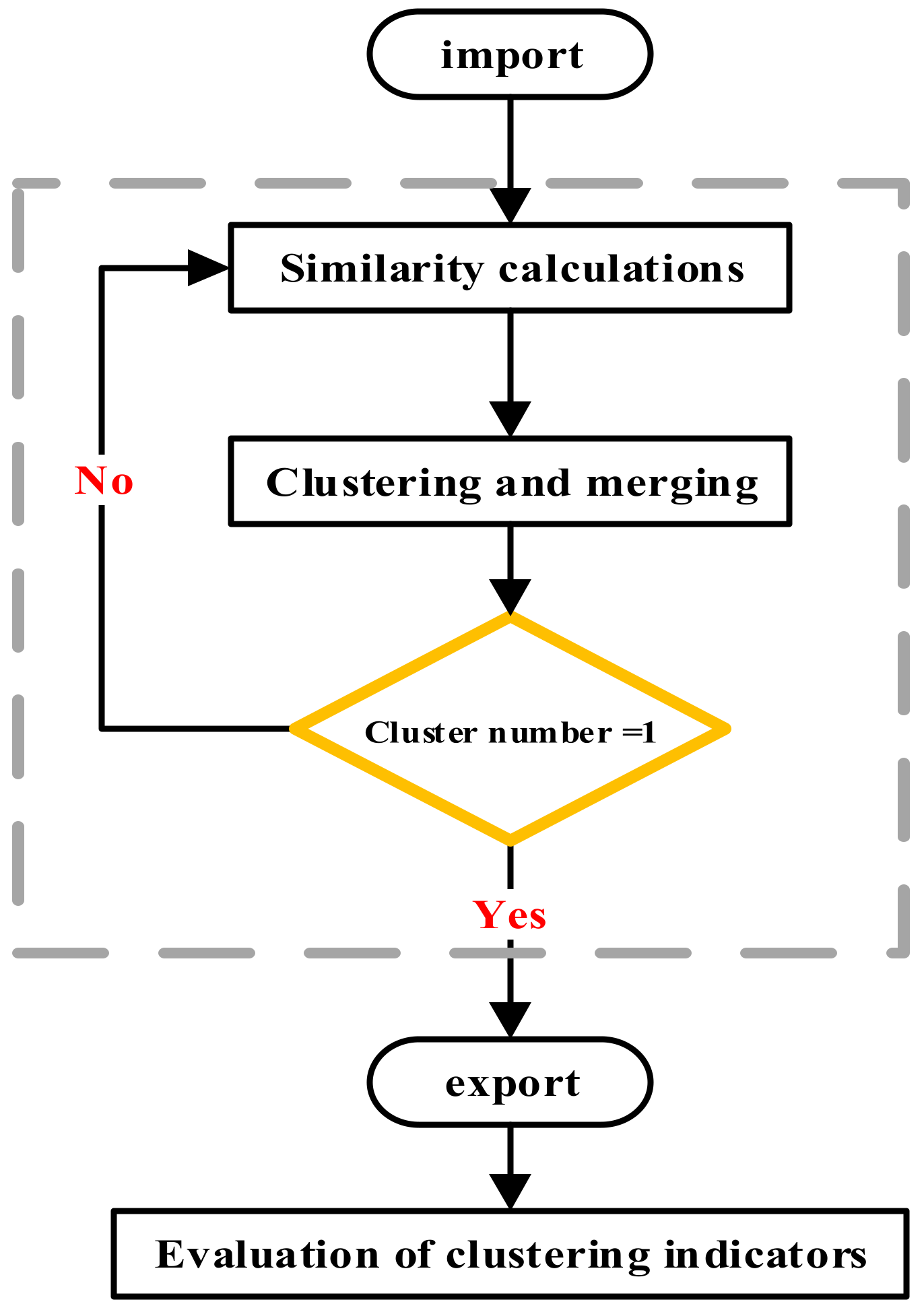
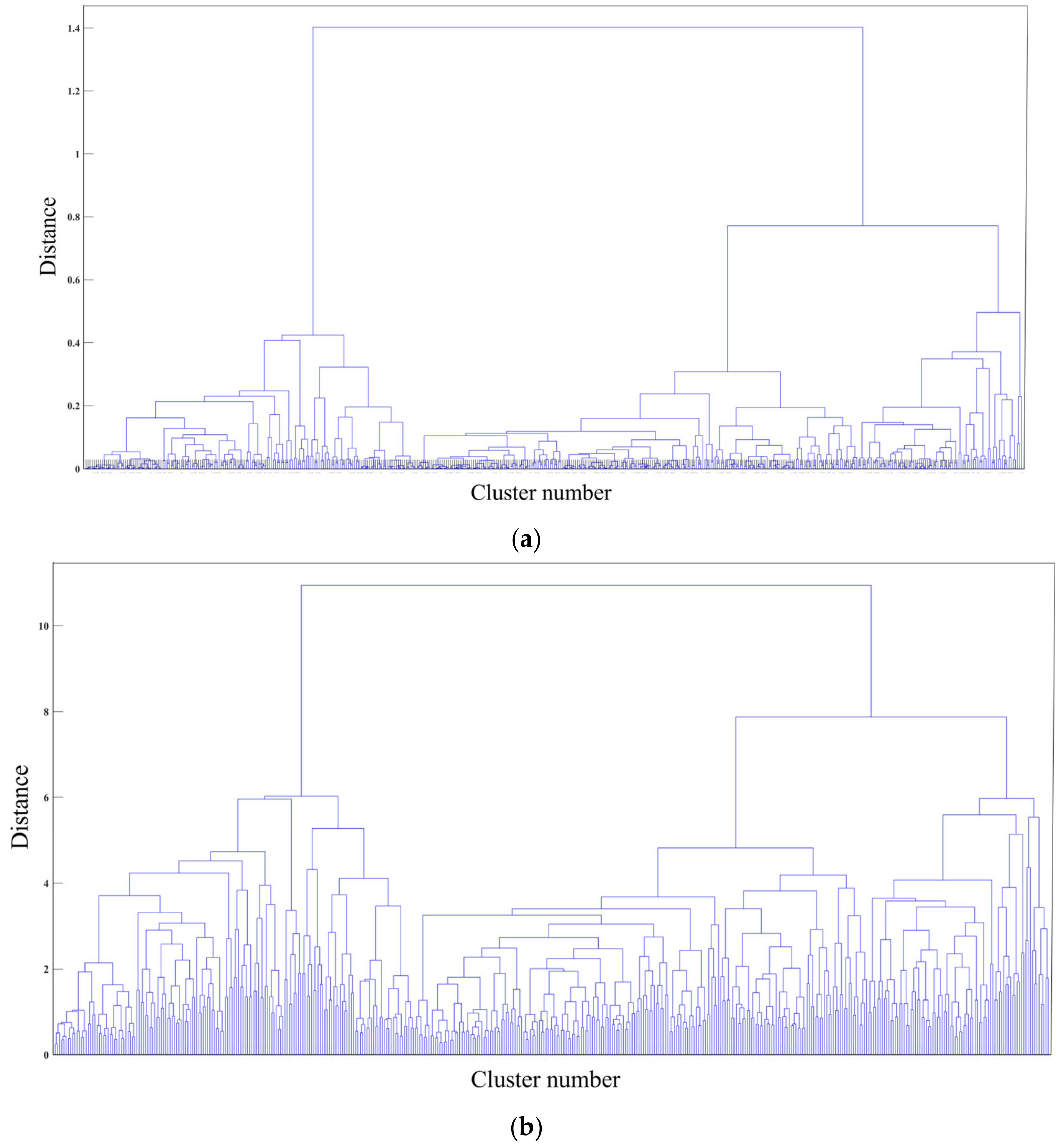
2.1.3. Agglomerative Hierarchical Clustering Analysis

The hierarchical clustering algorithm is a type of clustering algorithm based on similarity or distance measurement. Its main characteristic is to perform clustering by constructing a hierarchical structure of data points, which is presented in a tree-like structure, where each node represents a cluster. By comparing the similarity or distance between nodes, the hierarchical structure of the clusters can be determined. The hierarchical clustering algorithm used in this paper is the agglomerative hierarchical clustering algorithm, which is a bottom-up clustering method, where clusters can contain subclusters, and subclusters can contain even smaller subclusters [22]. In each successive iteration, the algorithm merges the closest pair of clusters that satisfy a similarity criterion until all data points are in one cluster. The average linkage clustering method is used in this process, which calculates all pairwise dissimilarities between elements in one cluster and elements in another cluster and considers the average of these dissimilarities as the distance between the two clusters. Finally, classification is performed based on the similarity measure between clusters.

Figure 2 shows the flow of cohesive hierarchical clustering. Firstly, the preprocessed wind speed profile data are input into it, and then the Euclidean distance and Pearson correlation coefficient are calculated to characterize the distance between the samples between the clusters. Then, the most similar or the smallest distance clusters are merged into a new cluster. If the number of clusters is not 1, the similarity calculation is re-performed. If the number of clusters is 1, the clustering result is visualized as a hierarchical clustering tree. Finally, the clustering result is output, and the clustering evaluation index is used to evaluate the agglomerative hierarchical clustering analysis.

The hierarchical clustering tree plays an important role in clustering analysis. It can usually directly display the inclusion relationship between upper and lower clusters, the importance of clusters, and the division between different clusters. It is an intuitive and convenient representation. It can understand the organization and relationship of data from the whole to the part. It is also flexible and does not need to determine the number of clusters in advance. Clustering results of different scales can be obtained by cutting the hierarchical clustering tree.

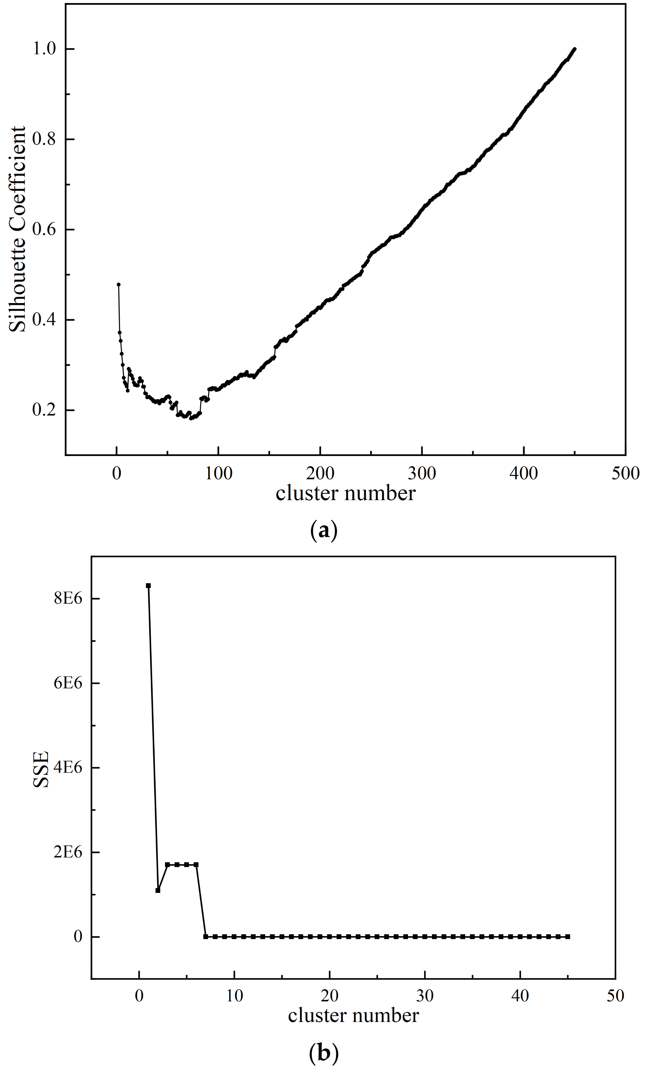
2.1.4. Validation of Clustering Results

After using the agglomerative hierarchical clustering algorithm for clustering analysis, it is necessary to evaluate the clustering results. This paper uses the silhouette coefficient [23] and sum of squared error to evaluate the clustering quality. In the sample set in this paper, the formula of the silhouette coefficient is the average value of the silhouette coefficient of all samples. The total silhouette coefficient $s_i$ of the cluster is expressed as follows:

$$S_i=\frac{1}{k}{\displaystyle \sum _{i=1}^k\frac{b_i-a_i}{\max \left(a_i,b_i\right)}}$$

(3)

In the formula, k is the total number of sample points, $a_i$ is the average distance between one sample and other samples in the cluster, and $b_i$ is the average distance between one sample and other cluster samples. The value range of the silhouette coefficient is between [−1, 1]. The larger the value is, the closer the cluster is. When the silhouette coefficient is 0, it means that there is cluster overlap. The closer it is to 1, the better the clustering quality is. The larger the silhouette coefficient is, the better the clustering effect is.

The sum of squares of clustering error is an important clustering evaluation index, which is of great significance in clustering analysis. The sum of squares of clustering error measures the sum of squares of the distance between each sample and the center of the cluster. In agglomerative hierarchical clustering, we can evaluate the quality of clustering by comparing the sum of squared errors of different clustering results. A smaller clustering error sum of squares indicates that the data points in the same cluster are more similar and the difference between different clusters is greater, which means that the clustering results are better. As the clustering iteration progresses, the sum of squared clustering error will gradually decrease until it finally stabilizes. The expression of the sum of squared clustering error is [24] as follows:

$$SSE={{\displaystyle \sum _i^k\left(d\right)}}^2$$

(4)

In the formula, d is the distance between each sample and its cluster center.

2.1.5. Selection of Clustering Results

Determining the optimal number of clusters is a key step in hierarchical clustering, which has a direct impact on the quality of clustering results. Comprehensive consideration of multiple indicators can more comprehensively evaluate the clustering results. In this paper, four indicators, the silhouette coefficient, sum of squares of clustering error, Calinski–Harabasz index, and Davies–Bouldin index, are used.

The validation of results includes the silhouette coefficient and the sum of squared errors in the results verification section. When the silhouette coefficient approaches 1, it indicates that the data points have a higher similarity to their own cluster and a lower dissimilarity to other clusters, suggesting better clustering effectiveness for that cluster. Therefore, the optimal number of clusters should be the one that maximizes the silhouette coefficient. At the same time, as the number of clusters increases, the sum of squared errors will gradually decrease. However, as the number of clusters further increases, the rate of decrease in the sum of squared errors will slow down, forming a clear inflection point. The number of clusters corresponding to this clear inflection point is the optimal number of clusters. In other words, the clustering result with a smaller sum of squared errors should be chosen as the best clustering result.

As the number of clusters increases, the Davies–Bouldin index and Calinski–Harabasz index change accordingly, and the optimal number of clusters can be determined by observing the changes in the Davies–Bouldin index and Calinski–Harabasz index; therefore, the Davies–Bouldin index and the Calinski–Harabasz index are suitable for judging the optimal number of clusters in agglomerative hierarchical clustering analysis. The Davies–Bouldin index essentially calculates the similarity between each cluster and its most similar clusters and then measures the whole clustering results by calculating the average value of all similarities. If the similarity between clusters is lower (the Davies–Bouldin index is lower), it means that the distance within the cluster is smaller and the distance between clusters is larger, so the clustering result is better, and vice versa. The calculation formula is as follows [25]:

$$DB=\frac{1}{k}{\displaystyle \sum _{i,j=1}^k\underset{i\ne j}{\max }\frac{s_i+s_j}{M_{ij}}}$$

(5)

In the above equation, DB is the abbreviation of Davies–Bouldin; k denotes the number of clusters; $s_i$ denotes the average distance from all sample points in the ith cluster to the center of the cluster; and $M_{ij}$ denotes the distance between the ith and jth clusters, that is, the distance between the centers of the two clusters. The Davies–Bouldin index measures the degree of balance between the tightness and separation of clusters, and the smaller the value of the index, the better the clustering results.

The Calinski–Harabasz index is also known as the variance ratio criterion. Its essence is the ratio of inter-cluster distance to intra-cluster distance. The compactness of the cluster is measured by calculating the square sum of the distance between each point in the cluster and the cluster center, and the separation is measured by calculating the square sum of the distance between the center point of the cluster and the center point of the data set. The judgment function is as follows [26]:

$$CH=\frac{BGSS}{k-1}/\frac{WGSS}{n-k}$$

(6)

In the formula, CH is the abbreviation of Calinski–Harabasz, n is the number of data set samples, k is the number of categories, BGSS is the between-group sum of squares, and WGSS is the within-group sum of squares. The larger the CH index is, the better the clustering effect is.

2.2. Wind Profile Fitting

After conducting agglomerative hierarchical clustering analysis on Typhoon Lekima, the optimal number of clusters was identified. Due to the fact that individual wind speed profiles hardly reflect the general patterns of wind speed profiles [12], numerous studies have opted for ensemble wind speed profiles for research purposes [27,28]. This study obtained ensemble wind speed profiles by averaging all 10 min average wind speed profiles at the same height and subsequently conducted fitting research.

The calculation of wind profiles is one of the main methods to study the change in wind speed. At present, the calculation models of wind profiles mainly include the Power-law model, Log-law model, Deaves–Harris model (D-H model), and Gryning model. In the near-surface layer, the wind profile is mainly affected by the roughness of the underlying surface, friction velocity, atmospheric stability, and other parameters.

The Power-law model is a functional form used to describe the average wind profile on the landform. Because of its simple form and convenient use, the model is widely used. At present, many countries, such as China and Japan, adopt the exponential rate model in their building codes for wind resistance design. The expression is as follows [29]:

$$U\left(z\right)=U\left(z_r\right){\left(\frac{z}{z_r}\right)}^{\alpha }$$

(7)

In the above formula, U(z) represents the wind speed at height z; U(z_r) represents the wind speed at reference height z_r, which is the reference wind speed; and α is the surface roughness index. In practice, α varies with wind speed, stability, and fitting height range [30]. However, the Power-law model still has some problems. The Power-law model is an empirical formula for the average wind speed, and it has not been developed with much reference to the real physical conditions of the atmospheric boundary layer. The model has the problem that it cannot satisfy the upper boundary condition or the lower boundary condition. It may not be able to describe the vertical distribution of low-level wind speed well. Cook et al. [31] pointed out that the Power-law model has the best fitting effect in the height range of 30~300 m.

According to the asymptotic similarity of the neutral atmospheric boundary layer, the Log-law model can be expressed as follows under neutral conditions [32]:

$$U\left(z\right)=\frac{u_{\ast }}{k}\ln \left(\frac{z}{z_0}\right)$$

(8)

In the above expression, U(z) denotes the wind speed at the effective height z; k is the von Karman constant, generally 0.4; z₀ denotes the roughness length of the ground, in m; and u* denotes the friction velocity. The effective height z is calculated as follows:

$$z=z\prime -z_d$$

(9)

where z′ is the height above ground and z_d is the zero-plane displacement, which is a function of surface roughness, height, and distribution. The Log-law model is ideal for describing the strong wind profile at the bottom of the atmosphere. The model can satisfy the minimum boundary conditions [33]. However, since only the surface roughness is considered and the height of the atmospheric boundary layer is not, the model is used to calculate the average wind speed above 100 m. The results will be relatively conservative. The research of Li et al. [34] also shows that the logarithmic rate model cannot describe the wind speed profile above 200 m.

The improved D-H model is based on the Log-law model, which improves the disadvantage that the Log-law model is only applicable to the near-surface layer. The improved model satisfies the upper boundary condition and the lower boundary condition at the same time and is suitable for the whole boundary layer. The improved D-H model is [35] as follows:

$$U\left(z\right)=\frac{u_{\ast }}{k}\left[\ln \left(\frac{z}{z_0}\right)+5.75\left(\frac{z}{h}\right)-1.88{\left(\frac{z}{h}\right)}^2-1.33{\left(\frac{z}{h}\right)}^3+0.25{\left(\frac{z}{h}\right)}^4\right]$$

(10)

In the above formula, h represents the height of the neutral boundary layer. The calculation of h is as follows:

$$h=\frac{u_{\ast }}{\beta f}$$

(11)

In the above formula, β represents the empirical parameter, generally 6 [6], and f is the Coriolis parameter, which is related to the latitude of the observation point and is generally 9.375 × 10⁻⁵/s.

When the height is more than 100 m, there is a certain deviation in the description of the wind profile by the logarithmic rate model. Based on a number of assumptions, Gryning et al. [36] proposed a wind profile model that can describe the entire boundary layer, and its expression under neutral conditions is

$$U\left(z\right)=\frac{u_{\ast }}{k}\left[\ln \left(\frac{z}{z_0}\right)+\frac{z}{L_{MBL,N}}-\frac{z}{h}\left(\frac{z}{2L_{MBL,N}}\right)\right]$$

(12)

In the above formula, L_MBL,_N is the total length scale under the neutral condition of the atmospheric boundary layer. The calculation of L_MBL,N is as follows:

$$L_{MBL,N}=\frac{u_{\ast }}{\left[-2\ln \left(\frac{u_{\ast }}{f{z}_0}\right)+55\right]f}$$

(13)

In addition, this paper also uses the empirical form of the inverse C-type wind speed profile to fit. The empirical form of the inverse C-type wind speed profile includes the Vickery model and the Snaiki and Wu model.

The empirical profile function proposed by Vickery et al. [37] is as follows:

$$U\left(z\right)=\frac{u_{\ast }}{k}\left[\ln \left(\frac{z}{z_0}\right)-\alpha {\left(\frac{z}{H^{\ast }}\right)}^n\right]$$

(14)

In the formula, u* is the friction velocity, k is the von Karman constant, generally 0.4, and a and n are considered as free parameters. In this paper, a takes 0.4, n takes 2.0, and H* is the boundary layer height parameter.

Snaiki and Wu [38] proposed various empirical forms of inverse C-type wind speed profiles, as shown below.

$$U\left(z\right)=\frac{u_{\ast }}{k}\left[\ln \left(\frac{z}{z_0}\right)+{\eta }_0\sin \left(\frac{z}{\delta }\right)\exp \left(-\frac{z}{\delta }\right)\right]$$

(15)

In the formula, η₀ is a constant, and δ is the height of the maximum wind speed, which is 190 m in this paper.

3. Data Acquisition

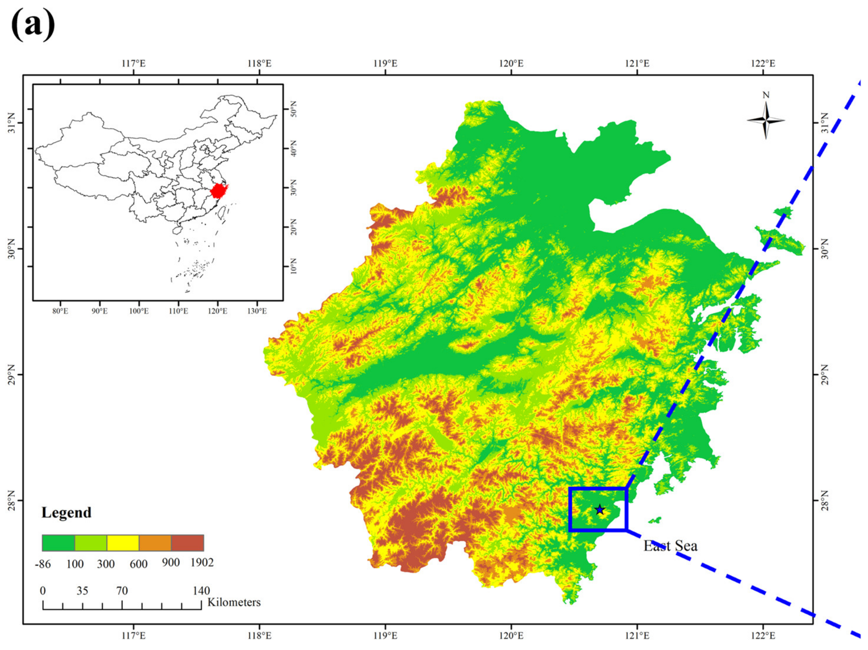
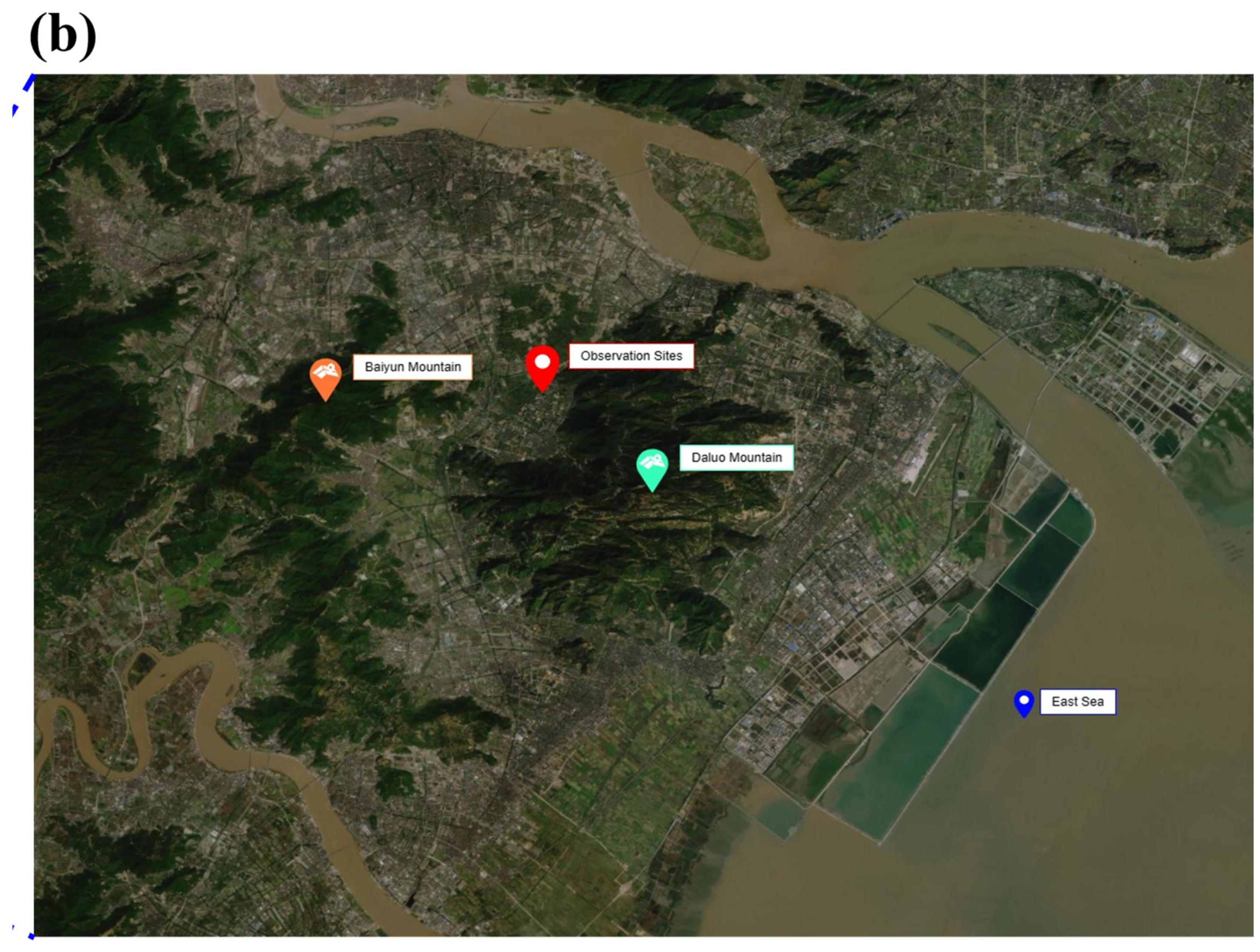
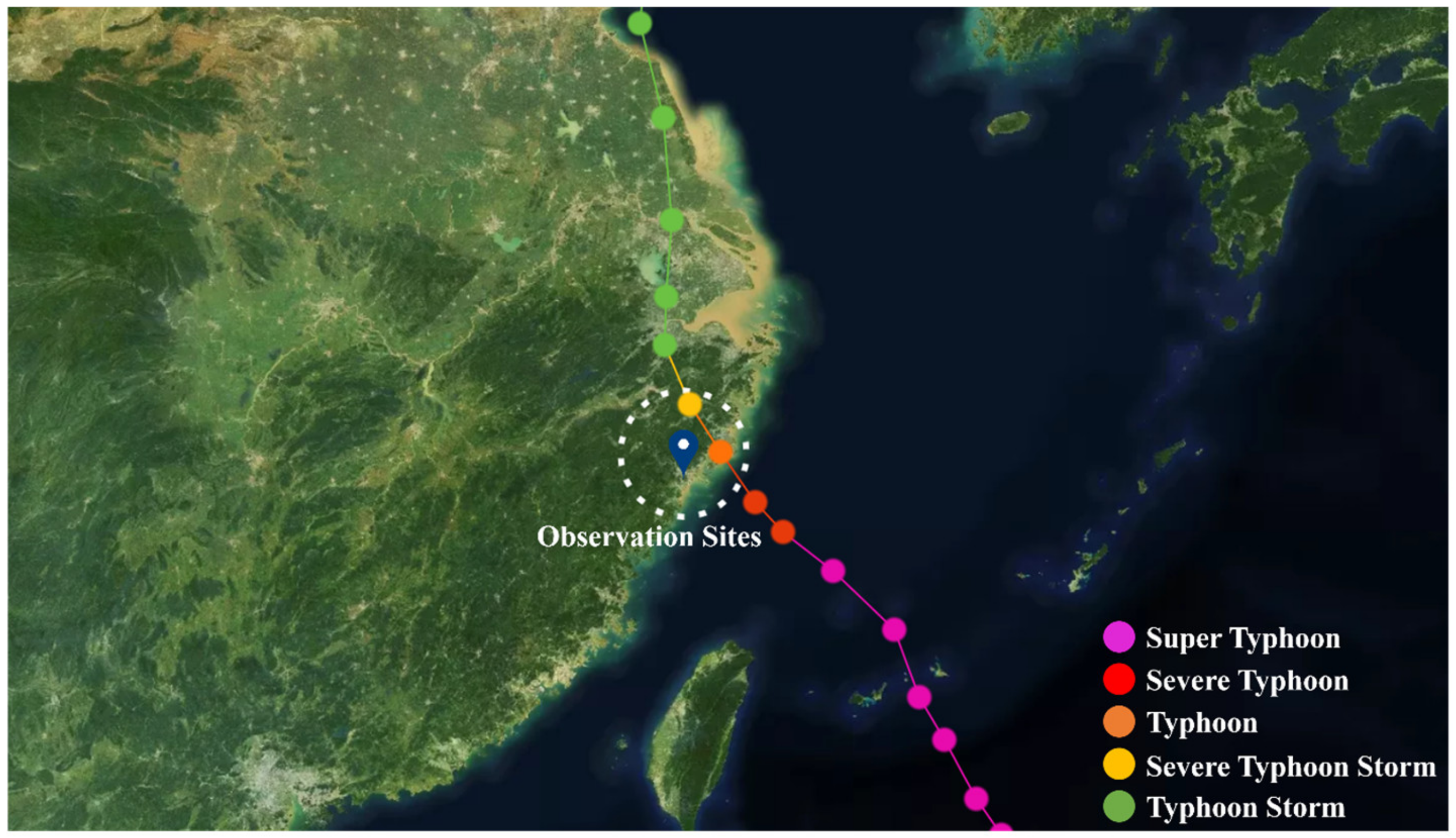
3.1. Observation Sites

The data observation site is located in Zhejiang Province, China, as shown in Figure 3a. The red part of the map of China in the upper left corner is located in Ouhai District, Wenzhou City, Zhejiang Province, as shown in Figure 3a. Wenzhou City is located in the southern part of Zhejiang Province, which is a typhoon-prone area. The topography of the observation site is as shown in Figure 3b. Furthermore, 2 km southeast of Daluo Mountain, the mountain trend is north–south, and the east–west branch is extended. The highest elevation of Daluo Mountain is 707.4 m, and the southeast side is about 17 km from the East China Sea coast. The northwest side is the open Sanyang Wetland, and the west side is Wenzhou City, which belongs to the suburbs of the city.

In Figure 4, the Typhoon Lekima path diagram is shown. The observation instrument measures the Typhoon Lekima at the observation point. The linear distance between the typhoon landing site and the observation point is about 82 km. During the typhoon landing, at 3:00 on 10 August 2019, the observation point is the closest to the typhoon center, about 70.8 km. At this time, the intensity level of the typhoon is strong typhoon level.

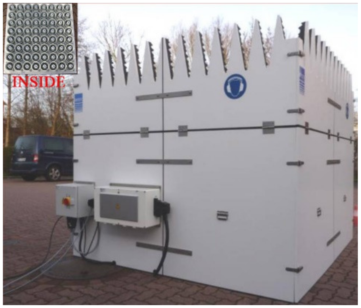
3.2. Observation Instrument

The observation instrument used in this study is the PCS.2000-64 mobile acoustic profile radar (SODAR) manufactured by METEK, Germany, as shown in Figure 5, which is used to measure continuous real-time three-dimensional vertical wind profiles and can also be used for remote measurements of wind speed, wind direction, and disturbances in the lower atmosphere, featuring convenient and flexible operation, easy setup, and mature analysis technology, and the specific technical specifications are shown in

Table 1. Acoustic sounder SODAR PCS2000-64 technical specifications.

Project	Value
Beam width	Typical 7~12° (depends on frequency)
Height resolution	Adjustable, 5 m ≤ ΔH ≤ 50 mIncrements ≥ 5 m, typical 10~30 m
Maximum measuring height	Nominally > 1500 m (not available in adverse weather conditions)
Minimum measuring height	≥15 m, adjustable, increment ≥5 m
Wind direction	0 to 360°
Wind direction accuracy	1~3° (wind speed > 5 m/s)3~5° (wind speed <5 m/s)
Vertical wind speed	−10~10 m/s
Horizontal wind components	±50 m/s
Vertical wind speed accuracy	0.03~0.1 m/s
Horizontal wind speed accuracy	0.1~0.3 m/s

. SODAR realizes remote measurements by transmitting acoustic signals into the atmosphere, and the backscattered acoustic signals can be used to invert wind speed and direction information by measuring the Doppler shift generated by the acoustic waves.

4. Data Preprocessing

4.1. Data Sample Control

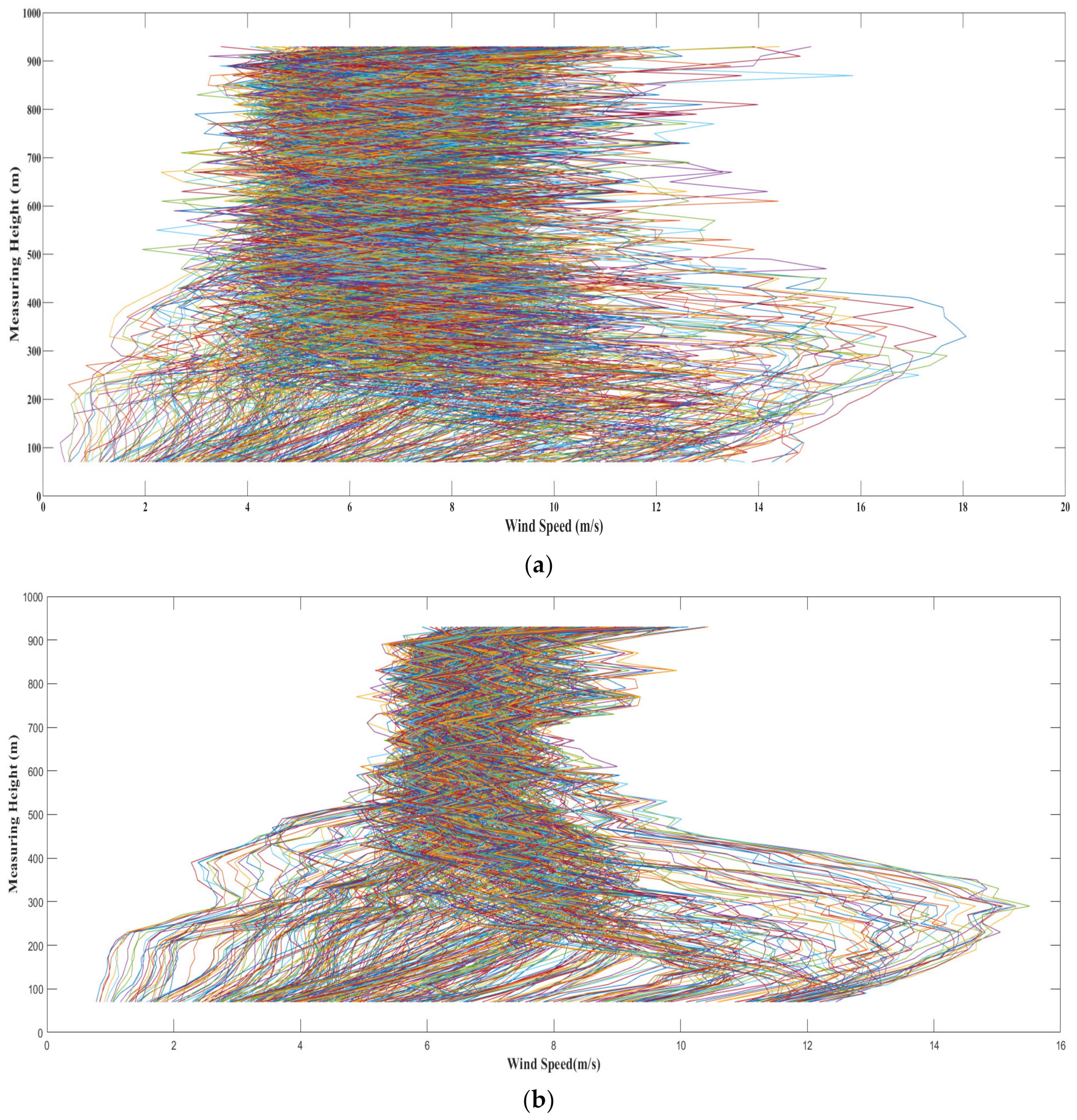
The measured data used in this paper are Typhoon Lekima-related data. The time length of Typhoon Lekima data is 7 August 2019, 5:00 pm—10 August 2019, 8:00 p.m., and the time is Chinese standard time (CST = UTC + 8 h). The reason for the length of time selected is that the intensity of Typhoon Lekima reached the typhoon level during this period. In the data processing, 10 min was selected as the average time interval, and the related factors of time and space were taken into account.

Due to weather and other reasons, some data quality is poor. In order to ensure the scientific and rigorous analysis results, this article has removed individual abnormal data. Due to the long total continuous observation time and large sample size, invalid samples were removed in data processing, which does not affect the overall validity and reliability of the data.The wind profile acoustic radar used in this paper has the advantage that the system state can be easily verified by the quality-related output variables (SNR, DA), which also include data availability (DA), signal-to-noise ratio (SNR), and error codes (ER) in the output data. Data availability is the ratio of used/successful instantaneous spectra. When the data availability is 0%, the data should be rejected, including anomalous data due to malfunction or signal transmission or anomalous data where wind speed and direction are outside the normal measurement range. The signal–noise ratio is the ratio of mean signal spectra to mean noise spectra. If the error code (ER) is 0%, the data should be rejected. The signal-to-noise ratio is the ratio of mean signal spectra/mean noise spectra. The error codes “01”, “02”, or “03” report rejected instantaneous spectra due to receiver saturation or broad band noise while the mean spectra are still normal, and the data are still fine. Error codes above “03” report rejected mean spectra, and the data should be rejected.

In Figure 6, the average wind speed contour map of Typhoon Lekima measured by wind profile acoustic radar with a time interval of 10 min is shown during the period from 17:00 on 7 August 2019 to 20:00 on 10 August 2019. The black dashed part of the figure indicates the time of landfall of Typhoon Lekima, which was 01:45 on 10 August 2019, and the landfall location of the typhoon was 86 km away from the observation point. In Figure 6, it is shown that the average wind speed peaked twice after the typhoon’s landfall, showing a trend of increasing, then decreasing, and then increasing, with the maximum average wind speed reaching 18 m/s. The total average wind speed after the passage of the typhoon was greater than that before the typhoon made landfall.

4.2. Data Smoothing

Figure 7a shows the average wind speed profile of the 10 min time interval of Typhoon Lekima without smoothing. It can be seen that there are many irregular fluctuations in the map. This is due to the fact that the measured data are greatly affected by the environment. Smoothing helps to reduce some random noise and fluctuations, thereby improving the interpretability of the profile data and revealing potential patterns and trends. For wind speed profile data, if there are a large number of random noises or irregular fluctuations, the smoothing method can eliminate these noises and extract the main features, so as to improve the effect of clustering analysis.

The data smoothing method used in this paper is the moving average method, which is a simple and effective smoothing method. By calculating the average value of wind speed observations in the window to smooth the data, it can effectively smooth out high-frequency noise or random fluctuations and help to reveal the potential patterns and periodic behaviors in the data. The moving average window size used in this paper is 10, as shown in Figure 7b. The moving-average-smoothed Typhoon Lekima’s 10 min average wind speed profile of 10 data points shows that the original random fluctuations basically disappeared, and the average wind speed profile data tended to be more stable. This makes the data easier to use in the next cluster analysis.

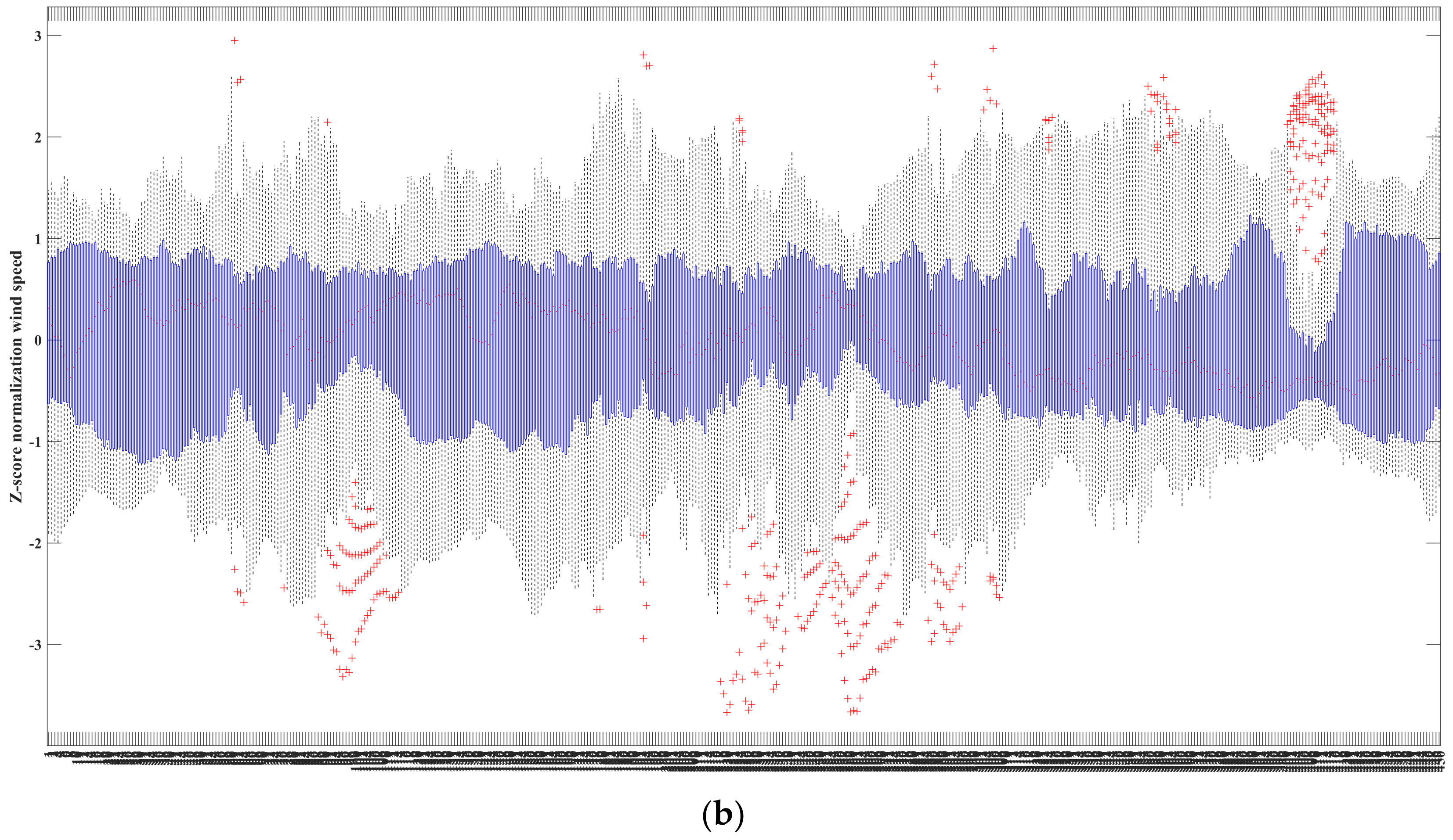
4.3. Data Standardization

Standardized data can eliminate the dimensional differences between different features so that the data can be compared on the same scale. In this paper, the wind speed profile needs to be clustered. In the clustering analysis, if the data are not standardized, the characteristics of the larger value may have a greater impact on the clustering results, resulting in the clustering results being biased towards the characteristics of the larger value. Through standardization, all features have the same importance and avoid this deviation.

For the agglomerative hierarchical clustering analysis of wind speed profiles, whether the data need to be standardized depends on the specific situation. In some cases, standardization may be necessary, while in other cases, it may not be possible. For instance, if the data of the wind speed profile have different magnitudes and units, or the distribution range of the data is quite different, then standardization can ensure that the contribution of the characteristics of different wind speed profiles to the clustering results is relatively balanced and avoids some characteristics dominating the clustering results. However, if the wind speed profile data already have similar dimensions and distributions, or the clustering algorithm itself is not sensitive to the scale of the data, then standardization may not be a necessary step. Therefore, whether it is necessary to standardize the data of wind speed profiles should be determined according to the specific situation. In this paper, we will use the method of drawing a box–line diagram to judge whether the data of wind speed profiles have similar dimensions and distributions and draw the box–line diagram of wind speed values at different heights to observe the dispersion degree and abnormal values of their distribution. By comparing the box plots at different heights, it can be inferred whether the data show different distribution characteristics. The collected wind speed values at different heights are grouped, and the relevant statistics corresponding to each height are calculated, such as the median, upper and lower quartiles, and possible outliers. If the box plot shows significant differences, including significant changes in the length, position, or shape of the box, it can be inferred that the wind speed data at different heights have different distribution characteristics. In addition, if there are a large number of outliers in the box plot, it indicates that there may be extreme wind speed values at some heights.

In Figure 8a, the 10 min time–distance wind speed box diagram of Typhoon Lekima is shown. In the box diagram, the blue represents the box, the box represents the upper and lower quartile range of the data, the middle line represents the median, and the upper and lower tentacles represent the overall distribution of the data. Any whiskers beyond 1.5 times the quartile distance are marked as outliers by symbols such as circles or asterisks. The above image is represented by a red cross. It can be seen that the box plot of the data in this paper shows obvious differences, indicating that the data have different distributions, so the data need to be standardized.

In this paper, the z-score normalization method is used to standardize the data. The z-score normalization is a common data normalization method. It realizes the normalization of the data by converting the data into a standard normal distribution with a mean of 0 and a standard deviation of 1. The formula used by the z-score normalization method is shown below [39].

$$z_i=\frac{x-\overline{x}}{\sigma }$$

(16)

where $z_i$ is the normalization results, $x$ is the value to be normalized, $\overline{x}$ is the average value, and σ is the standard deviation. In Figure 8b above, the box plot of the normalized wind speed data at 10 min for Typhoon Lekima is shown. It can be clearly seen that the median of the data is distributed around 0 after z-score normalization, which is close to 0. The box indicates that the interquartile range of the data is close to 2, and the upper quartile and lower quartile of the data are distributed between −1 and 1. Most of the upper and lower limits in the box plot are close to 3 and −3, respectively. It can be considered that the effect of z-score normalization processing is better.

5. Results and Discussion

5.1. Results of Agglomerative Hierarchical Clustering Analysis

In this paper, the hierarchical clustering tree of the Typhoon Lekima 10 min time–distance wind speed profile was obtained by agglomerative hierarchical clustering analysis. Figure 9a is a hierarchical clustering tree based on the Pearson correlation coefficient, and Figure 9b is a hierarchical clustering tree based on the Euclidean distance. It can be clearly seen that all samples are finally concentrated in a cluster, and finally, the appropriate typical wind speed profile samples can be selected according to the optimal clustering number.

After the clustering analysis is completed, the clustering results need to be evaluated. In this paper, the evaluation index is the sum of the contour coefficient and the clustering error square. The following Figure 10a shows the silhouette coefficient map after the hierarchical clustering analysis. It can be seen that the silhouette coefficient decreases first and then increases with the increase in the number of clusters. After all data aggregation is complete, the silhouette coefficient reaches 1, which indicates that this cohesive hierarchical clustering analysis is better and the clustering results are more compact. As shown in Figure 10b, it can be clearly seen that the sum of squared errors is very large at the beginning of clustering, with values over 1,000,000. As the clustering progresses, the sum of squared errors gradually decreases. When the number of clusters increases, the sum of squared errors gradually approaches 0, indicating that the aggregated hierarchical clustering is effective. Considering the two clustering evaluation indexes of the silhouette coefficient and clustering error sum of squares, this agglomerative hierarchical clustering analysis has a certain level of scientific knowledge, which provides support for the next clustering optimal result selection.

After the evaluation of the clustering results was completed, this paper chose the optimal clustering results, which were combined with the silhouette coefficient and the sum of the square of the clustering error, and the CH index and the DB index. In Figure 11b below, the Calinski–Harabasz index and the Davies–Bouldin index are plotted. It can be seen that when the number of clusters is three, the CH index reaches 561.3, but the DB index is in a high state at this time. However, when the number of clusters is two, the CH index is only different by 4.39 from when the number of clusters was three, while the DB index is 0.12 lower than that when the number of clusters was three, so two clusters are more appropriate. Considering the four indicators, it is decided to select the optimal clustering number of this agglomerative hierarchical clustering as two.

5.2. Typical Wind Profile

Figure 12a,b, respectively, represent two optimal clusters and the preliminary fitting results based on the sample composition trends. In this study, cluster I wind profiles shown in Figure 12a are named as “cluster 1 type”, while cluster II wind profiles in Figure 12b are named as “cluster 2 type”. It can be observed that the average wind speed profiles of cluster type 1 show an increasing trend followed by a decrease and then stabilization as the measurement height increases, while the average wind speed profiles of cluster type 2 exhibit an initial increase followed by gradual stabilization. Both average wind speed profiles show significant differences at lower altitudes but exhibit similarities above 500 m, gradually stabilizing with minimal fluctuations. As shown in Figure 13, there are distinct differences in the wind speed profiles of the two categories below 500 m, with both cluster 1 and cluster 2 wind speed profiles effectively reflecting the characteristics of the sample wind speed profiles.

After obtaining two typical average wind speed profiles, cluster 1 type and cluster 2 type, it is necessary to further study the average wind speed profile characteristics of these two forms. The following is the model fitting of the two forms of wind speed profiles. The fitting height of this wind profile is 300 m. The measured height of 50 m is the reference height, and the measured wind speed at 50 m height is the reference wind speed. In order to quantify the fitting degree of the six wind speed profile models to the observed wind profile, this paper uses the R² test as the evaluation index of the goodness of fit test of the wind speed profile, and the value of R² ranges from 0 to 1; a value closer to 1 indicates a better fitting effect, and a value closer to 0 indicates a poor fitting effect.

5.3. Results of the Wind Profile Fitting Analysis

In this paper, the measured wind speed profile of cluster 1 type shows an anti-C shape. In Figure 14a, the mean wind profile of cluster 1 is compared with the two model wind profiles. It can be seen that below 300 m, the horizontal wind speed is 8–11 m/s, and the average wind speed first increases and then decreases. The average wind profile shows an anti-C shape. There is a low-level jet phenomenon near the vertical height of about 50–300 m. Kepert et al. [40] show that the low-level jet is a common feature of the mean wind profile of the tropical cyclone boundary layer. The maximum mean wind speed appears near the height of about 200 m, which is consistent with the peak wind speed found by Gunter and Schroeder around 200 m, while Powell et al. [41] found that the maximum mean wind speed height of an Atlantic hurricane near the ground is 500 m, which is much higher than the cluster 1 wind profile. Both the Vickery model and the Snaiki and Wu model can effectively describe the cluster 1 wind profile of the wind speed profile, as shown in Figure 14a. The relevant fitting parameters and goodness of fit results of the cluster 1 wind profile are shown in

Table 2. Cluster 1 and 2 fitting parameters of wind speed profile.

Typhoon Samples	Vickery						Snaiki and Wu
Cluster 1	u*	z0	a	n	H*	R2	u*	z0	η0		R2
	1.11	2.34	0.4	2.0	153.49	0.992	0.21	7.69 × 10−4	24.88		0.987
Cluster 2	Power-law model		Log-law model			Deaves–Harris model			Gryning model
	α	R2	u*	z0	R2	u*	z0	R2	u*	z0	R2
	0.33	0.987	0.587	6.041	0.971	0.278	0.873	0.984	0.266	0.762	0.984

. It can be seen that the Vickery model can better describe the cluster 1 wind profile than the Snaiki and Wu model at the height of 130 m-270 m, and the overall goodness of fit of the Vickery model is also greater than that of the Snaiki and Wu model.

As shown in Figure 14b, the comparison of cluster 2 average wind profiles with four model wind profiles reveals that below the height of 300 m, the horizontal average wind speed ranges from 3 to 6 m/s, showing a gradual increasing trend that also rises with vertical height. The fitting parameters and goodness of fit results for the cluster 2 wind profile are presented in Table 2. It can be observed that the Power-law, Log-law, Deaves–Harris (D-H), and Gryning models all exhibit good fitting for the average wind profile below the fitted heights, with goodness of fit values exceeding 0.97. Specifically, the Power-law model demonstrates the best fitting performance at heights of 50–70 m, 110 m, 250 m, and 290 m, while the Log-law model performs best at 90 m but shows poor fitting performance beyond 100 m. The D-H model exhibits the best fitting performance at heights of 130 m and 270 m, and the Gryning model performs best at heights of 150–230 m. Overall, the Power-law model shows good fitting performance at heights of 50–150 m and 250–300 m, while the Gryning model performs better at heights of 150–250 m. Additionally, as the height exceeds 250 m, the fitting performance of all four models gradually deteriorates.

6. Conclusions

In this paper, the moving acoustic profile radar deployed in Ouhai District, Wenzhou City, Zhejiang Province, was used to observe the average wind profile data of Typhoon Lekima in the vertical range of 50–1000 m from the ground in 2019. Based on the observed data, the average wind profile with different characteristics was clustered by using the agglomerative hierarchical clustering analysis algorithm, and two typical average wind profiles were obtained. The model fitting analysis of the classified samples was performed to study the characteristics of the average wind profile of Typhoon Lekima and to provide a reference for the study of different typhoon average wind profiles. The main findings and results of this study are as follows:

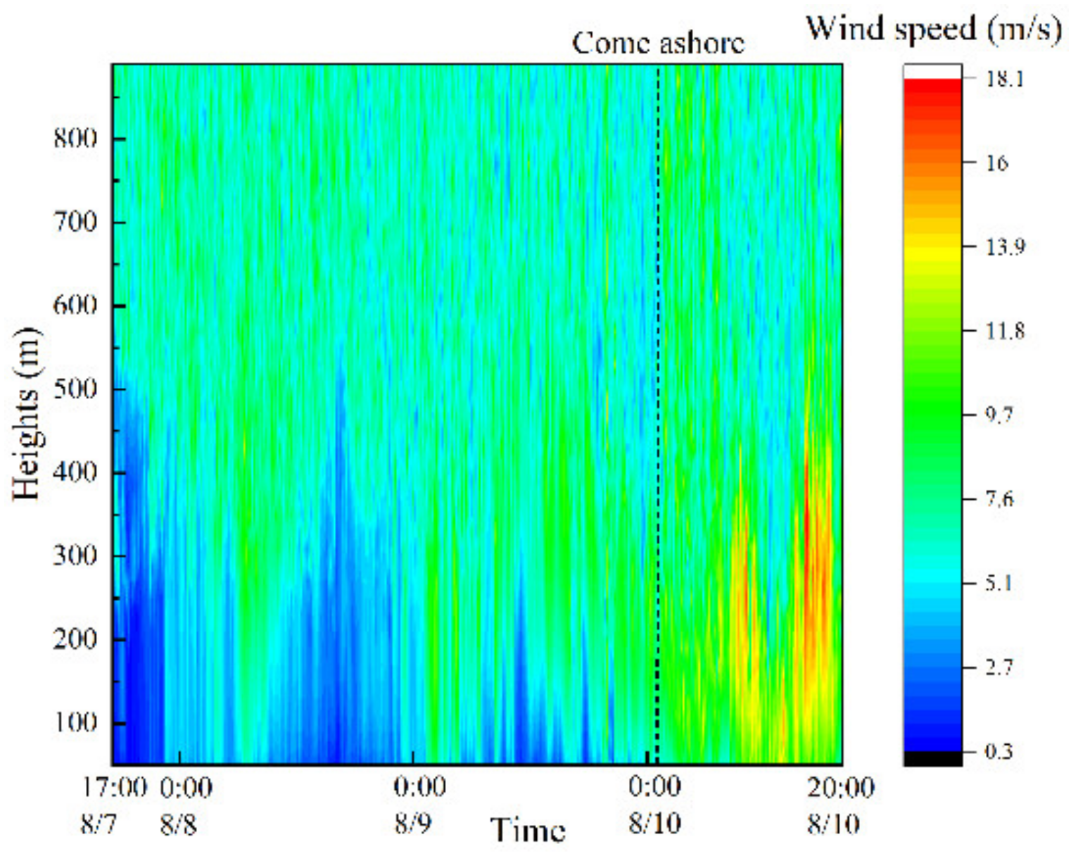
• Since the measured data of Typhoon Lekima are not suitable for direct clustering analysis, this paper smoothes the measured data and uses the z-score normalization method to standardize the data, which reveals the potential patterns and trends of the data. Then, the agglomerative hierarchical clustering analysis method is used to effectively classify Typhoon Lekima. The Euclidean distance and Pearson correlation coefficient are used as measurement criteria, and the contour coefficient and sum of squared clustering error are used as clustering evaluation indexes. The results show that the clustering effect is good. Finally, the optimal number of clusters is selected by combining the contour coefficient and the sum of squared clustering error, the CH index, and the DB index.
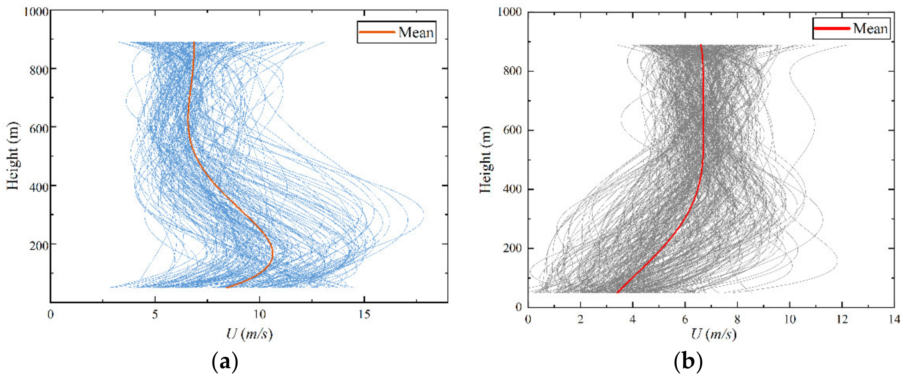
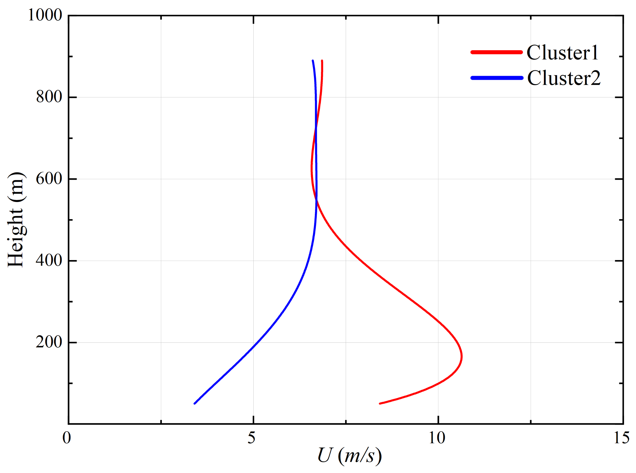
• Based on the agglomerative hierarchical clustering analysis, the mean wind profile of Typhoon Lekima can be divided into two types. In this paper, the two typical mean wind profiles are named cluster 1 and cluster 2. For cluster 2, the wind speed gradually increases with increasing height and then gradually stabilizes. For cluster 1, there is an obvious low-level jet phenomenon, and the wind speed first increases, then decreases, and then slightly increases with the increase in height.
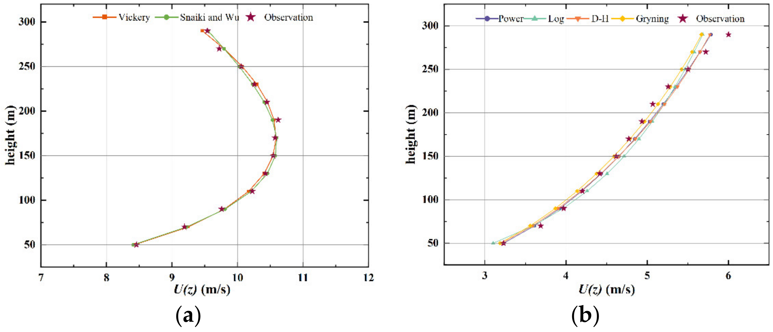
• After cluster analysis, this paper also carried out fitting processing. The average wind speed profile of cluster 1 shows an inverse C shape, and there is a low-level jet phenomenon near the vertical height of about 50–300 m, and the average wind speed appears near the height of 200 m. The empirical form of the wind speed profile used for fitting in this paper is the Vickery model and the Snaiki and Wu model. In terms of the overall fitting effect, the Vickery model is superior to the Snaiki and Wu model. Especially at the height of 130–270 m, the Vickery model can better describe the average wind profile of cluster 1.
• The average wind profile of cluster 2 is fitted by four calculation models: the Power-law model, Log-law model, Deaves–Harris model, and Gryning model. In general, the fitting effects of the four models are good, and the coefficient of the goodness of fit can reach more than 0.97. Among them, the Power-law model has a better fitting effect when the height is 50–150 m and 250–300 m, and the Gryning model has a better fitting effect when the height is 150–250 m. It is worth noting that when the height is greater than 250 m, the fitting effect of the four models on the cluster 2 mean wind profile gradually deteriorates with the increase in height.

The conclusions of this paper can provide a reference for near-surface typhoon modeling in wind field numerical simulation and the setting of wind tunnel test environments in structural wind engineering. In practical engineering applications, it can strengthen the understanding of the average wind profile characteristics of the boundary layer under strong typhoons in coastal areas and promote the wind resistance design of high-rise building structures.

It is worth noting that only a single typhoon was used for the cluster analysis in this study. In the future, more measured typhoon data are needed to further improve the conclusions of this study. It is also possible to classify the observed typhoon data by wind speed and then perform cluster analysis. This will provide more specific conclusions. In addition, the problem of typhoon wind direction can be comprehensively considered to further promote the application of the average wind profile under typhoon conditions in structural wind engineering and to provide a theoretical basis for the wind resistance of high-rise and super-high-rise structures.

References

1. Ciarlatani, M.F.; Huang, Z.; Philips, D.; Gorlé, C. Investigation of Peak Wind Loading on a High-Rise Building in the Atmospheric Boundary Layer Using Large-Eddy Simulations. J. Wind Eng. Ind. Aerodyn. 2023, 236, 105408. [Google Scholar] [CrossRef]
2. Ricci, M.; Patruno, L.; Kalkman, I.; De Miranda, S.; Blocken, B. Towards LES as a Design Tool: Wind Loads Assessment on a High-Rise Building. J. Wind Eng. Ind. Aerodyn. 2018, 180, 1–18. [Google Scholar] [CrossRef]
3. Dongmei, H.; Shiqing, H.; Xuhui, H.; Xue, Z. Prediction of Wind Loads on High-Rise Building Using a BP Neural Network Combined with POD. J. Wind Eng. Ind. Aerodyn. 2017, 170, 1–17. [Google Scholar] [CrossRef]
4. Mohammadi, A.; Azizinamini, A.; Griffis, L.; Irwin, P. Performance Assessment of an Existing 47-Story High-Rise Building under Extreme Wind Loads. J. Struct. Eng. 2019, 145, 04018232. [Google Scholar] [CrossRef]
5. Zheng, X.-W.; Li, H.-N.; Yang, Y.-B.; Li, G.; Huo, L.-S.; Liu, Y. Damage Risk Assessment of a High-Rise Building against Multihazard of Earthquake and Strong Wind with Recorded Data. Eng. Struct. 2019, 200, 109697. [Google Scholar] [CrossRef]
6. Tieleman, H.W. Strong Wind Observations in the Atmospheric Surface Layer. J. Wind Eng. Ind. Aerodyn. 2008, 96, 41–77. [Google Scholar] [CrossRef]
7. Song, L.; Chen, W.; Wang, B.; Zhi, S.; Liu, A. Characteristics of Wind Profiles in the Landfalling Typhoon Boundary Layer. J. Wind Eng. Ind. Aerodyn. 2016, 149, 77–88. [Google Scholar] [CrossRef]
8. Lin, L.; Chen, K.; Xia, D.; Wang, H.; Hu, H.; He, F. Analysis on the Wind Characteristics under Typhoon Climate at the Southeast Coast of China. J. Wind Eng. Ind. Aerodyn. 2018, 182, 37–48. [Google Scholar] [CrossRef]
9. Han, Z.; Wang, X.; Tang, Y.; Yue, C.; Ao, X. Characteristic Analysis of Measured Winds under Typhoon Chan-hom and Normal Climate at Xujiahui in Shanghai. Meteorol. Sci. Technol. 2020, 48, 529–536. Available online: https://jglobal.jst.go.jp/en/detail?JGLOBAL_ID=202002232011931521 (accessed on 3 June 2024).
10. Chen, T.; Fu, J.Y.; Chan, P.W.; He, Y.C.; Liu, A.M.; Zhou, W. Wind Characteristics in Typhoon Boundary Layer at Coastal Areas Observed via a Lidar Profiler. J. Wind Eng. Ind. Aerodyn. 2023, 232, 105253. [Google Scholar] [CrossRef]
11. Tamura, Y.; Iwatani, Y.; Hibi, K.; Suda, K.; Nakamura, O.; Maruyama, T.; Ishibashi, R. Profiles of Mean Wind Speeds and Vertical Turbulence Intensities Measured at Seashore and Two Inland Sites Using Doppler Sodars. J. Wind Eng. Ind. Aerodyn. 2007, 95, 411–427. [Google Scholar] [CrossRef]
12. Franklin, J.L.; Black, M.L.; Valde, K. GPS Dropwindsonde Wind Profiles in Hurricanes and Their Operational Implications. Weather Forecast. 2003, 18, 32–44. [Google Scholar] [CrossRef]
13. Shu, Z.R.; Li, Q.S.; He, Y.C.; Chan, P.W. Vertical Wind Profiles for Typhoon, Monsoon and Thunderstorm Winds. J. Wind Eng. Ind. Aerodyn. 2017, 168, 190–199. [Google Scholar] [CrossRef]
14. Tse, K.T.; Li, S.W.; Chan, P.W.; Mok, H.Y.; Weerasuriya, A.U. Wind Profile Observations in Tropical Cyclone Events Using Wind-Profilers and Doppler SODARs. J. Wind Eng. Ind. Aerodyn. 2013, 115, 93–103. [Google Scholar] [CrossRef]
15. Beu, C.M.L.; Landulfo, E. Machine Learning-Based Estimate of The Wind Speed Over Complex Terrain Using the LSTM Recurrent Neural Network. Wind Energy Sci. Discuss. 2023, 2023, 1–31. [Google Scholar]
16. Li, F.; Xie, Z.; Yang, Y.; Yu, X. Investigations of Synoptic Wind Profile Patterns in Complex Urban Areas Based on LiDAR Measurements. Build. Environ. 2023, 242, 110573. [Google Scholar] [CrossRef]
17. Schelbergen, M.; Kalverla, P.C.; Schmehl, R.; Watson, S.J. Clustering Wind Profile Shapes to Estimate Airborne Wind Energy Production. Wind Energy Sci. 2020, 5, 1097–1120. [Google Scholar] [CrossRef]
18. Mohandes, M.; Rehman, S.; Rahman, S.M. Estimation of Wind Speed Profile Using Adaptive Neuro-Fuzzy Inference System (ANFIS). Appl. Energy 2011, 88, 4024–4032. [Google Scholar] [CrossRef]
19. Liu, Z.; Zheng, C.; Wu, Y.; Song, Y. Investigation on Characteristics of Thousand-Meter Height Wind Profiles at Non-Tropical Cyclone Prone Areas Based on Field Measurement. Build. Environ. 2018, 130, 62–73. [Google Scholar] [CrossRef]
20. Burlando, M.; Antonelli, M.; Ratto, C.F. Mesoscale Wind Climate Analysis: Identification of Anemological Regions and Wind Regimes. Int. J. Climatol. 2008, 28, 629–641. [Google Scholar] [CrossRef]
21. Janse Van Vuuren, C.Y.; Vermeulen, H.J. Clustering of Wind Resource Data for the South African Renewable Energy Development Zones. J. Energy South. Afr. 2019, 30, 126–143. [Google Scholar] [CrossRef]
22. Müllner, D. Modern Hierarchical, Agglomerative Clustering Algorithms. arXiv 2011, arXiv:1109.2378. [Google Scholar]
23. Kim, B.; Kim, J.; Yi, G. Analysis of Clustering Evaluation Considering Features of Item Response Data Using Data Mining Technique for Setting Cut-Off Scores. Symmetry 2017, 9, 62. [Google Scholar] [CrossRef]
24. Nainggolan, R.; Perangin-angin, R.; Simarmata, E.; Tarigan, A.F. Improved the Performance of the K-Means Cluster Using the Sum of Squared Error (SSE) Optimized by Using the Elbow Method. J. Phys. Conf. Ser. 2019, 1361, 012015. [Google Scholar] [CrossRef]
25. Davies, D.L.; Bouldin, D.W. A Cluster Separation Measure. IEEE Trans. Pattern Anal. Mach. Intell. 1979, PAMI-1, 224–227. [Google Scholar] [CrossRef]
26. Calinski, T.; Harabasz, J. A Dendrite Method for Cluster Analysis. Commun. Stat.—Theory Methods 1974, 3, 1–27. [Google Scholar] [CrossRef]
27. Powell, M.D.; Vickery, P.J.; Reinhold, T.A. Reduced Drag Coefficient for High Wind Speeds in Tropical Cyclones. Nature 2003, 422, 279–283. [Google Scholar] [CrossRef] [PubMed]
28. Giammanco, I.M.; Schroeder, J.L.; Powell, M.D. GPS Dropwindsonde and WSR-88D Observations of Tropical Cyclone Vertical Wind Profiles and Their Characteristics. Weather Forecast. 2013, 28, 77–99. [Google Scholar] [CrossRef]
29. Davenport, A.G. Rationale for Determining Design Wind Velocities. J. Struct. Div. 1960, 86, 39–68. [Google Scholar] [CrossRef]
30. Li, Q.S.; Zhi, L.; Hu, F. Field Monitoring of Boundary Layer Wind Characteristics in Urban Area. Wind Struct. 2009, 12, 553–574. [Google Scholar] [CrossRef]
31. Cook, N.J. The Deaves and Harris ABL Model Applied to Heterogeneous Terrain. J. Wind Eng. Ind. Aerodyn. 1997, 66, 197–214. [Google Scholar] [CrossRef]
32. Kustas, W.P.; Brutsaert, W. Wind Profile Constants in a Neutral Atmospheric Boundary Layer over Complex Terrain. Bound.-Layer Meteorol. 1986, 34, 35–54. [Google Scholar] [CrossRef]
33. Simiu, E.; Scanlan, R.H. Wind Effects on Structures: Fundamentals and Applications to Design; John Wiley: New York, NY, USA, 1996; Volume 688. [Google Scholar]
34. Li, Q.S.; Zhi, L.; Hu, F. Boundary Layer Wind Structure from Observations on a 325m Tower. J. Wind Eng. Ind. Aerodyn. 2010, 98, 818–832. [Google Scholar] [CrossRef]
35. Deaves, D. A Mathematical Model of the Structure of Strong Winds. CIRIA Rep. 76 Const. Ind. Res. Inf. Assoc. 1978. [Google Scholar]
36. Gryning, S.-E.; Batchvarova, E.; Brümmer, B.; Jørgensen, H.; Larsen, S. On the Extension of the Wind Profile over Homogeneous Terrain beyond the Surface Boundary Layer. Bound.-Layer Meteorol. 2007, 124, 251–268. [Google Scholar] [CrossRef]
37. Vickery, P.J.; Wadhera, D.; Powell, M.D.; Chen, Y. A Hurricane Boundary Layer and Wind Field Model for Use in Engineering Applications. J. Appl. Meteorol. Climatol. 2009, 48, 381–405. [Google Scholar] [CrossRef]
38. Snaiki, R.; Wu, T. A Semi-Empirical Model for Mean Wind Velocity Profile of Landfalling Hurricane Boundary Layers. J. Wind Eng. Ind. Aerodyn. 2018, 180, 249–261. [Google Scholar] [CrossRef]
39. Imron, M.A.; Prasetyo, B. Improving Algorithm Accuracy K-Nearest Neighbor Using Z-Score Normalization and Particle Swarm Optimization to Predict Customer Churn. J. Soft Comput. Explor. 2020, 1, 56–62. [Google Scholar] [CrossRef]
40. Kepert, J.; Wang, Y. The Dynamics of Boundary Layer Jets within the Tropical Cyclone Core. Part II: Nonlinear Enhancement. J. Atmos. Sci. 2001, 58, 2485–2501. [Google Scholar] [CrossRef]
41. Gunter, W.S.; Schroeder, J.L. High-Resolution Full-Scale Measurements of Thunderstorm Outflow Winds. J. Wind Eng. Ind. Aerodyn. 2015, 138, 13–26. [Google Scholar] [CrossRef]
Figure 1. Technical route.
Atmosphere 15 00708 g001
Figure 2. Flow chart of agglomerative hierarchical cluster analysis.
Atmosphere 15 00708 g002
Figure 3. Location of observation points: (a) geographical map and (b) topographical map.
Atmosphere 15 00708 g003aAtmosphere 15 00708 g003b
Figure 4. Typhoon Lekima track map.
Atmosphere 15 00708 g004
Figure 5. The SODAR PCS.2000-64.
Atmosphere 15 00708 g005
Figure 6. The measured 10 min average wind speed of Typhoon Lekima.
Atmosphere 15 00708 g006
Figure 7. The average wind speed profile (a) at 10 min of Typhoon Lekima before smoothing and (b) after moving average smoothing of 10 data points.
Atmosphere 15 00708 g007
Figure 8. Typhoon Lekima 10 min wind speed box plot (a) without standardization and (b) after standardization.
Atmosphere 15 00708 g008aAtmosphere 15 00708 g008b
Figure 9. The hierarchical clustering tree (a) of wind speed profile at 10 min time interval of Typhoon Lekima based on Pearson correlation coefficient and (b) based on Euclidean distance.
Atmosphere 15 00708 g009
Figure 10. Clustering index evaluation: (a) silhouette coefficient and (b) clustering error sum of squares.
Atmosphere 15 00708 g010
Figure 11. The best clustering number selection: (a) SSE and silhouette coefficient and (b) Calinski–Harabasz index and Davies–Bouldin index.
Atmosphere 15 00708 g011
Figure 12. Preliminary fitting results after wind speed profile clustering: (a) cluster 1 and samples and (b) cluster 1 and samples.
Atmosphere 15 00708 g012
Figure 13. Different types of wind speed profiles.
Atmosphere 15 00708 g013
Figure 14. Comparison of average wind profile and model wind profile: (a) cluster 1 type and (b) cluster 2 type.
Atmosphere 15 00708 g014