Abstract
By deploying machine learning (ML) and deep learning (DL) algorithms, we address the problem of smell event modelling in the Pittsburgh metropolitan area. We use the Smell Pittsburgh dataset to develop a model that can reflect the relation between bad smell events and industrial pollutants in a specific urban territory. The initial dataset resulted from crowd-sourcing citizen reports using a mobile phone application, which we categorised in a binary matter (existence or absence of smell events). We investigate the mapping of smell data with air pollution levels that were recorded by a reference station located in the southeastern area of the city. The initial dataset is processed and evaluated to produce an updated dataset, which is used as an input to assess various ML and DL models for modelling smell events. The models utilise a set of air quality and climate data to associate them with a smell event to investigate to what extent these data correlate with unpleasant odours in the Pittsburgh metropolitan area. The model results are satisfactory, reaching an accuracy of 69.6, with ML models mostly outperforming DL models. This work also demonstrates the feasibility of combining environmental modelling with crowd-sourced information, which may be adopted in other cities when relevant data are available.
1. Introduction
Air pollution significantly affects quality of life and is one of the major environmental concerns in urban areas. The city under study (Pittsburgh, Pennsylvania, USA) has a history of air pollution due to the presence of various industries such as steel production. Many industrial activities are conducted in the greater metropolitan area currently, with this case study focusing on the Allegheny County area, which is primarily impacted by the operation of a petroleum refinery unit associated with the release of sulphur oxides [1]. In this research, we are specifically interested in modelling the relationships between odour experiences and air pollutants using the Smell Pittsburgh dataset. Smell Pittsburgh (https://smellpgh.org/, accessed on 18 May 2024) is a mobile application for crowd-sourcing odour reports, originally designed to empower citizens to address air pollution issues [2]. The application was deployed in 2016 and is still an ongoing project.
We employ two different types of data in our analysis: air pollution measurements (from a relevant monitoring station) and smell reports. By modelling the relationship between these two, we aim to inspect how local people’s living experiences are related to air pollution. The insights obtained from this research can potentially inform local community members and stakeholders to improve air quality in areas with similar air pollution characteristics. The research procedure we establish may also motivate other municipalities to conduct similar research to assess the impact of air pollution on citizens and urban environment.
Previous research has applied machine learning (ML) on the Smell Pittsburgh dataset to predict the presence of odour in an 8h range for the Pittsburgh region using air quality sensor measurements [2]. Here, we take a different perspective. Instead of modelling the entire Pittsburgh region, we narrowed the scale down to inspect the viability to model a local region where a reference air quality monitoring station is located. This approach allows us to better understand the performance of ML and deep learning (DL) models at a finer geographical resolution.
2. Literature Review
Air quality modelling, especially in urban areas, employs various simulation approaches to initially mimic the behaviour and the dynamics of the urban atmosphere and then to investigate the possible relationships between air pollution sources and other environmental factors and their impact on air quality. Developments in computer systems over the last twenty years have enabled a rapid increase in the use of numerical simulation models that treat urban air pollution as a system. The main objective of this discipline is the detailed simulation of the spatial and temporal distribution of air pollutants, from source emissions to the determination of the level of pollutant concentrations in a ‘virtual’ microenvironment that is part of the wider urban environment [3].
Different approaches have been developed to model concentrations of atmospheric pollutants that are harmful to human health [4,5]. Several of them are based on mathematical methods that determine the concentration of pollutants in the air when there is a lack of sufficient data [6]. Other approaches are based on available data from monitoring stations, low-cost instruments [7] and citizen inputs [8]. If sufficient data are available, some of the most popular approaches are ML and DL to explore the correlations between different data [9]. Some of the most popular ML algorithms are Random Forest, Support Vector Regression, Gradient Boosting, Multiple Linear Regression, and Artificial Neural Networks, which can find a pattern in complex, unstructured and non-linear data in air pollution datasets [10]. In this research, we focus on exploring the possible correlation of odour data with air pollution levels and climate data, deploying ML and DL algorithms.
Modelling the olfactory mechanism is one of the most challenging problems as it is the least understood of all the human senses [11]. This is primarily due to the subjective nature of the sense of smell. However, in recent years, there has been significant progress in this research area. Models have been developed in order to determine odour concentration levels at various receptor points around a source of pollution/odour. Atmospheric dispersion models like AERMOD have been deployed to simulate the dispersion of chemical compounds that produce unpleasant odours [12].
Recent studies provide evidence that odour modelling is feasible and, in some cases, a quite effective tool in the assessment of the environmental impact that is caused by odour emissions, especially if adequate spatial data (of a high resolution) are available [13]. Odours can be associated with the presence of high levels of gaseous pollutant concentrations [14]. Dispersion modelling has been suggested to study the relationship between odours and certain air pollutant emissions [15]. Nevertheless, only a few works attempted to produce ML/DL models or develop numerical modelling algorithms that correlate odour data with the presence of air pollution [16,17]. Thus, this study aims to contribute to the available scientific literature.
Citizens living in highly industrialised urban centres can experience unpleasant odours associated with anthropogenic activities that cause air quality pollution [18]. In this case, citizen observations can be valuable for research, which links to the citizen science area that engages people in data collection [8]. Such crowd-sourced data can provide information for training ML/DL models to tackle local concerns and investigate the patterns of complex problems [19]. In the field of odour sensing, citizen science shows promising results in providing solutions to address urban air pollution issues [20].
3. Materials and Methods
3.1. Smell Pittsburgh Dataset
The Smell Pittsburgh dataset was developed by the CREATE Lab at Carnegie Mellon University and contains five years of smell reports and sensor measurement data from November 2016 (dataset—https://github.com/CMU-CREATE-Lab/smell-pittsburgh-prediction, accessed on 18 May 2024). The dataset was published under the Creative Commons Zero (CC0) license with a CSV file structure. A previous work used an earlier version of the dataset that contains two years of data for pollution pattern analysis and predictive modelling [2].
The configuration of the database used in this research was based on the following procedure: Smell report data are collected from Pittsburgh citizens using a mobile application (its interface is displayed in Figure 1). The input process includes severity ratings from 1 to 5, with 5 being the most and 1 the least strong smell. A text description of the smell source is also available, accompanying symptoms, geographical locations of the reports (in latitude and longitude), timestamps upon submission, and zip codes. To protect the privacy of the users, geographical locations (latitude and longitude) are skewed, but the zip codes reflect the location in general. Also, the user information is excluded intentionally for privacy concerns, which means that it is unknown whether one user submitted smell reports multiple times within a certain short time window.
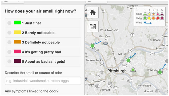
Figure 1.
Smell Pittsburgh mobile phone app. The right image is showing a map of Pittsburgh’s urban area. Triangles represent smell reports and circles represent PM2.5 levels. The image in the left provides an overview of the smell report app screen, where the user can have a clear view of the data that can be reported in the app.
3.2. Air Quality Measurements
The air quality and climate data were obtained through the United States Environmental Protection Agency (EPA). The EPA provides such information from a reference station (EPA, pre-generated data files: https://aqs.epa.gov/aqsweb/airdata/download_files.html, accessed on 18 May 2024) (Allegheny Monitoring Station) located in the Pittsburgh metropolitan area. Climate data are also available, such as the wind direction/speed and temperature. Each record also has an associated timestamp. Data are available in annual, monthly, and hourly formats for the 1980–2023 period.
3.3. Selection of the Geographic Region
Several studies for determining the environmental burden of a region conclude that selecting a specific metropolitan region can yield results that better reflect actual conditions [21].
In this study, we selected a specific urban zone in the southeast Pittsburgh metropolitan area (as shown in Figure 2); our choice was based on the following criteria:
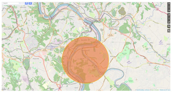
Figure 2.
Location of Allegheny air quality monitoring station in the Pittsburgh metropolitan area and schematic representation of the study radius, i.e., the area in which the smell data were collected (orange circle). It is noted that some zip codes incorporated in the study may fall outside this circle.
- i.
- Existence of abundant odour data from this specific area (that will evidently provide sufficient information to train ML and DL models).
- ii.
- Existence of an air quality reference monitoring station to ensure data quality.
- iii.
- Relative homogeneity of urban morphology (to control the noise in the data).
The area that meets all these requirements is in southern Pittsburgh (Allegheny County) and it was therefore selected to be the focus of this study. Furthermore, there are industrial activities near the selected zone, which may contribute to air quality degradation. Hence, many reports regarding strong odours are expected. The study region is the circular zone around the reference station and is characterised by rich vegetation (grass and trees) and a low building density. Based on the area’s morphology, elevated levels of air pollution may be more associated with the presence and activity of industries rather than other anthropogenic factors, such as increased traffic congestion.
We chose 8 km as the radius of the study area to ensure homogeneity in terms of urban density, green zones, and other features of urban morphology. It is worth noting that the study zone depicted in Figure 2 does not fully reflect the study area nor is it the most accurate representation possible. The reason behind this is that we selected smell data on the basis of zip codes, which correspond to various area shapes, so it is not possible to derive a study area that is a perfect circle.
3.4. Data Pre-Processing
To transform the original smell report dataset into a dataset that would best fit into our ML and DL models, we have devised the following pipeline. Firstly, we have chosen the period that we would retrieve the smell data, and this was 2018–2022. We then selected the odour data from citizen inputs based on the zip codes in our study region. The zip codes that were chosen were the following: 15025, 15034, 15037, 15045, 15047, 15088, 15104, 15110, 15120, 15122, 15123, 15131, 15132, 15133, 15135, 15137.
Next, we removed rows containing zero or non-numeric values from the dataset. As the reports of the citizens were in an exact time format (e.g., 09:47) and the time data from the reference station are in an hourly format, we rounded the time to the nearest hour (e.g., 10:00) to associate the data from smell reports dataset with the data from the EPA.
We then decided to transform the smell related data into a binary format. We aggregated the severe smell reports near the reference station into “odour episodes”, representing a pungent odour event. We decided to group all the smell reports with a value ranging from 0 to 3 as 0: no smell episode, and values in the range of 4–5 as 1: a smell episode. Although reports with values of 1–3 indicate the presence of odour, and we could have included these classes as smell episodes, we considered this categorisation as suboptimal. This comes from the definition of different levels of odour nuisance in the mobile application (Smell Pittsburgh). Value 3 is defined as an overall acceptable (in terms of annoyance) smell. We therefore chose this categorisation to ensure that there is definitely (as objectively as possible) an unpleasant odour in the air, which is generally and not subjectively perceived. This binary coding was also made to simplify the task that the models will have to undertake, and an additional reasoning was that the research question can be narrowed to: “Are the citizens of Pittsburgh experiencing bad odour in the air related to low air quality or not?”. In this scope, we can simplify and group the smell categories to the above two categories.
We also decided to process the daily data of smell reports to reflect their relationship with possible activities (on weekdays opposed to weekends), attributing values of 1–7 for each day (1 = Monday…, 7 = Sunday). We also included the skewed latitude and longitude values in our analysis, as they were processed in the same way; as far as the training of the models is concerned, they can provide a sufficient input. Finally, we did not incorporate in our analysis the column that had comments from the citizens, as we did not develop a model that could process natural language features. This would be quite interesting, but more suitable for another type of analysis compared to ours, which is focused on numerical data analysis.
Snapshots of the data resulting from the pre-processing phase are presented in Table 1a,b in order for the reader to have a clearer understanding of the features that have been incorporated in the model training procedure. The total number of smell reports recorded in the mobile application for each year is summarised in Table 2, where different rates of citizen engagement are displayed for different years. We then processed the data from the reference station. We used PM25, PM10 and SO2 for air quality data, and temperature, wind speed and wind direction for climate data. While particulate matter is not directly related to bad odours, as it is seemingly odourless, it may be associated with sources (industrial or agricultural) that produce bad odours. However, relevant research provides evidence of a positive association between long-term PM2.5 exposure and odour identification [22].

Table 1.
Dataset after pre-processing. (a) Part 1—xxx and yyy present undisclosed data. (b) Part 2—continuation of Table 1a.
Table 2.
Number of bad smell reports over the course of 2018−2022.
Furthermore, sulphur dioxide is a gas with a strong, irritating and pungent odour used in a variety of workplaces (i.e., in inorganic and petrochemical industries) [23], making it an ideal choice for the needs of our research. On top of that, the Smell Pittsburgh mobile application provides citizens with the option to provide a comment with their smell report. Although an analysis of these comments was not performed in this research, the citizens’ comments were also considered in the formulation of our research strategy. In many of these comments, the citizens mentioned the smell of “rotten eggs”, a smell commonly associated with the presence of high concentrations of hydrogen sulphide, so this was an additional indicator to incorporate sulphur dioxide into the analysis. Pollutants like benzene, toluene, etc., that are strongly related to the presence of strong/unpleasant odours would provide a higher accuracy to the model; however, we were limited to the data that were available from the EPA, so we proceeded to perform the analysis with the aforementioned gaseous compounds.
The selected climate data can be linked to the presence of bad odours. The direction of the wind, for example, can be a decisive factor in the presence of unpleasant odours in an area if it blows from the direction of the source. In addition, the temperature was incorporated in the analysis, although the relationship between odour concentration and temperature is quite complex and not a straightforward mechanism [14].
The ambient temperature is a meteorological parameter that could influence odour attention. Research provides evidence that there is a correlation between temperature levels and odour concentrations [24]. However, this is not the case for all the parameters that influence odour concentration, like odour dispersion, where the temperature has a smaller effect [12]. Based on the above, a final decision on whether to incorporate temperature in our analysis was based on the effect of its presence on the results. As the results with temperature in the training features were better, we decided to keep it in the analysis.
We chose to process all the available pollutants to investigate their potential relationship with unpleasant odours. Unpleasant smells have historically been linked to potential risks to human health. Malodours emitted by industrial activities, animal production facilities and other human activities are known to lead to complaints regarding eye and nose irritation, coughs, headaches, etc. [14]. These symptoms, being similar to those caused by elevated levels of air pollution, may establish a link between unpleasant odours and poor air quality. We then deleted all the rows that did not contain a value for any of the features.
After the dataset of the air quality was ready, we begun the procedure of associating the two datasets. Therefore, we chose the smell reports that were available for each hour. To ensure that the smell data are closely connected to the reference station data, we opted to keep the smell reports that had the smallest distance to the reference station.
3.5. The Post-Processed Dataset
The final dataset consisted of 9085 rows and 12 columns (Day, Hour Val, Latitude (skewed), Longitude (skewed), Zip code, PM25, PM10, SO2, Temperature, Wind direction, and Wind speed as model input features and Smell event as the model output variable).
The resulting database contained data from January 2018 to January 2022 (Table 3). The data were not evenly distributed across the years. This is expected, as the level of commitment of the citizens fluctuated over the time frame of our study, while the emergence of the COVID-19 pandemic may have had an influence.
Table 3.
Model performance using 10-fold cross-validation. Model performance metrics are averaged across all 10 folds.
Each year provided over 1000 training instances, so it is safe to assume that the dataset provides a representative picture of odour episodes over the years. The fact that the number of smell reports did not decrease over the years, but rather remains stable or even increases, is an indicator that citizens’ interest in this issue remains strong and that they have confidence that this odour recording effort will provide some positive results in the future. Among the data points, 5598 (61.6%) of them include odour episodes (presence of a bad smell). As can be seen, there is an uneven distribution between the odour and non-odour data. However, we have chosen not to interfere with this distribution to create a balanced dataset so that the model predictions reflect the existing real-life picture. All the data pre-processing was performed with R programming language.
3.6. ML and DL Architecture and Training Hyperparameters
To fit a model Y = F(X), we use the column ‘Smell event’ as the response variable (Y) and the columns of Day, Hour val, Latitude (skewed), Longitude (skewed), Zip code, PM25, PM10, SO2, Temperature, Wind direction and Wind speed as the predictors (X). The models used in this study employ ML algorithms as well as DL algorithms. In the case of ML, we employed Multi-layer Perceptron (MLP), Support Vector Machine (SVM), Random Forest (RF), Gradient Boost (GB) and X-Gradient Boost (xGB) algorithms. We also tested the implementation of DL networks like long short-term memory (LSTM) and two variations of LSTM: stacked and bidirectional and Recurrent Neural Networks (RNNs). Our algorithm selection considered previous work in the field [25] as well as our intention to investigate different model approaches.
In the case of MLP, we constructed a model consisting of 100 hidden layers, deploying the ReLU (Rectified Linear Unit) activation function in each layer. The learning rate was set to 0.001 and the stochastic-gradient-based Adam optimiser was chosen for neuron weight optimisation. Concerning the GB model, the learning rate was set to 0.1. The maximum depth of individual trees within the ensemble was set to 5. The boosting stages/iterations that were performed were 100. Finally, the minimum number of samples required to split an internal node was set to 10.
For the XGB model, the learning rate was set to 0.1 and the maximum depth was set to 7. The boosting stages that this model required were 50. In the SVM model, the Kernel function that yielded the best results was sigmoid. We also chose to set a gamma value of 0.1 to define the influence that each training example had on the model. For the RF model, we used a total number of 300 trees in the ensemble (forest). The number of splits that each decision tree was allowed to make (maximum depth) was set to none, combined with a minimum split rate of 10. The function we deployed to measure the quality of the splits was Gini. Finally, we chose not to run jobs in parallel in the training process.
For the LSTM model, we used one LSTM layer with 64 LSTM units. The sigmoid activation function was employed, which is suitable for binary classification problems, like the one we are investigating in this study. We also used binary cross-entropy as the loss function to determine the difference between model outcomes and the actual values. The optimiser used in this model was Adam; the learning rate was set to 0.001 and the number of training epochs was set to 10. In the case of the stacked LSTM model, we created two LSTM layers, with the first having 64 LSTM units and the second having 32 LSTM units. The rest of the parameters were the same as in the case of the simple LSTM model.
For the bidirectional LSTM model, which allows the LSTM layer to learn in both the forward and backward directions, we used a single LSTM layer with 64 neurons. The rest of the hyperparameters were the same as in the other two LSTM variations. Finally, in the RNN model, we made use of a simple RNN layer with 64 RNN units (neurons).
The activation function was sigmoid, the loss function was binary cross-entropy and the optimiser was once more Adam. The learning rate was set to 0.001 and the number of training epochs that yielded the best results was 10. We implemented these models using Python programming language, the scikit-learn ML library for ML models and TensorFlow/Keras libraries for DL models.
3.7. Model Validation and Performance Evaluation
We used 10-fold cross-validation to evaluate the models’ performance. In this setting, the input space (dataset) was divided into ten equally sized folds, where nine folds were used for training the model and the remaining one-fold was used for testing. This process was repeated 10 times (each time leaving a different fold out) until all the (different) folds were used for testing the model. To decide which model had the best overall performance, we have chosen the following evaluation metrics:
- Accuracy (the fraction of successful forecasts to total forecasts).
- Recall (ratio of positive values successfully classified as positive divided by the total positive values).
- Precision (ratio of the successful classification of positive values divided by the total projections categorised as positive by the model).
- F-score (harmonic mean of previously calculated precision and recall).
Moving forward, we normalised the data of columns that were used as training inputs. The normalisation technique we employed in this case study is Min–Max normalisation (feature scaling). This method rescales each feature in the dataset to a fixed range, which was set to between 0 and 1 in our case (which is also the most common approach). This normalisation manages to preserve the original data relationships while ensuring uniformity in the scale across all the normalised features.
We opted to normalise all the features to limit the influence of outlier values in the model training to have an unbiased learning. This can have a serious (positive) impact on algorithms/models like Gradient Boosting, which are distance-based. Also, since we have values of different variables (such as hours, days, pollutant concentrations and wind intensity), it is necessary to adjust them all to a common scale so that we avoid the phenomenon of one column (i.e., feature) having a greater influence on training due to increased weights, which will result from its higher values [26].
4. Results
The model results are summarised in Table 3, where the model evaluation metrics are reported for each model type used. In addition, in Figure 3, the Receiver Operating Characteristic (ROC) curve as well as the relevant Area Under the Curve (AUC) are reported for the three ML models in our study, as well as the feature ranking resulting from the RF algorithm.
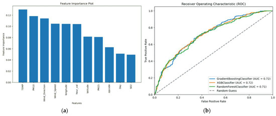
Figure 3.
(a) How the Random Forest model evaluates the importance of features used for its training; (b) AUC curve for the three ML models of this study. (Random Forest Classifier, Gradient Boost Classifier and X Gradient Boost Classifier). The closer the curve is on the upper left corner of the diagram space, the better quality of the predictions. We observe that these three models showcase similar performances, so their differences can be spotted in other performance metrics.
The overall performance of the models was found to be satisfactory in model performance metrics, although some values, like the 99.6% recall of SVM that may seem to be an indicator of a particularly high performance, do not reflect the whole picture of the performance, as this is not the case for the rest of the metrics and SVM does not outperform the rest of the models. Based on the overall performance in all the metrics, GB and RF models proved to perform better on our data. These two models provide better performance among the ML models, especially for Precision and F-score. XGB is very close to these performances as well, although somewhat lower compared to GB. The overall picture, however, is that all the ML models were able to fit our data and could model the occurrence of a smell episode with high precision. The similar performance of the models is also reflected in the AUC curve, where three models (GB, XGB and RF) have almost identical curves, which indicates the good fit of these models to the available data.
DL models, on the other hand, provide satisfactory results, especially for the Recall metric; however, their performance was inferior to that of the ML models. Despite testing various architectures of LSTM and RNNs, the results obtained do not demonstrate significant differences and therefore are not considered to be the best model solution for the problem under study. Nevertheless, their performance is more than satisfactory and might have been superior if we had more training data, as DL models tend to perform better when more training data are available.
5. Discussion
In this section, we present some of the most interesting findings from the study results. We comment on the performance of the models and attempt to interpret some outcomes that are of interest regarding the environmental part of the study.
Figure 3 shows the performance of the RF model and provides insight into the features that the models consider as important. The most important features are found to be the temperature, PM10 and wind direction. These results seem to be consistent with the nature of this study. As far as the temperature is concerned, it influences the volatility and diffusion of odour molecules in the air. Therefore, it is expected to play an important role in whether an unpleasant odour is perceived or not. It is worth noting that wind direction has higher significance values compared to the values of the air pollutant concentrations, reflecting a quite important finding of the study: wind blowing from a congruent direction is associated with certain human activities, possibly industrial. This finding is supported by the existence of pollution sources in the area, which contribute (to a greater or lesser extent) to the presence of odours. In addition, the importance of PM10 may be attributed to the simultaneous production of this pollutant as well as of odorous substances from the same anthropogenic activity. An additional finding is that all models demonstrate a sufficient capability to infer both smell events and non-smell events. As our dataset is unbalanced, with more training instances for smell events, we were expecting the models to perform better in these cases. This behaviour outlines the ability of ML/DL models to fit particularly complex data, such as the dataset developed for this case study.
The models may perform better if there is more information within the available dataset that would allow them to better “learn” the relationships between environmental data and odour episodes and therefore model the latter in a more effective way. However, this condition is part of the problem we are tackling, as we are bounded by the availability of data. Therefore, it is necessary to develop methods that also take this into account and can produce highly accurate model results. A future approach to the problem may incorporate more advanced feature engineering and refinements to the model architecture. Moreover, the availability of additional features is expected to improve model outcomes if they adequately reflect odour generation and dispersion mechanisms.
Another technique not explored in this study is training the models on a more balanced dataset, i.e., a database where there is a balanced the number of odour and non-odour episodes. In this case study, the number of odour episodes was about twice as high as the number of non-odour cases, so one might expect that a more evenly balanced dataset would yield better results. We did not pursue this perspective here, as we believe that the resulting data would not be sufficient for satisfactory model training. In the future, when data availability will allow it, such a research perspective may yield the expected results.
We display the ROC curve of the three different models in Figure 3. This curve captures the ratio of odour episode predictions that were confirmed relative to all odour episodes estimated by the model. The slope of the curve depicts the complexity of the data on which the models were deployed to find a pattern. The slope of the curve indicates that there is clear room for improvement. This performance of the models reinforces the need to explore other methods of pre-processing the data or even explore other ML models to find an approach that gives a more satisfactory answer to the problem faced in this study.
Finally, we address the inferior performance of DL models compared to ML models. Although we conducted extensive tests on a range of different network architectures, the performance of the DL models failed to approach that of the ML models, although they are still satisfactory. While DL models have immense potential, they may not be the ideal solution when applied to numerical data and when aiming to solve a binary classification problem with not a lot of data available, such as the dataset utilised in this study.
6. Conclusions
Crowd-sourced information is important in environmental modelling, as citizen-contributed data reflect living experiences, which are not captured by sensor measurements. Although the collected data were odour-related, which are challenging to model, it turned out that there is room for development of scientific research, which, based on this type of data, could yield significant results, like in this case study.
Our research shows that citizen-contributed odour data, while important, can be noisy and difficult to model. The results indicate that it remains a big challenge to map citizens’ experiences to sensor measurements using DL and ML techniques; however, with the right strategy of feature engineering, pre-processing and model fine-tuning, satisfactory results can be achieved. The exploration of the models for estimating smell events by processing air quality, climate and georeferenced data (even with a skewed latitude and longitude, as in our case) seems encouraging at first sight, as the results are quite promising. The models’ performance underlines the challenging nature of the modelling problem we faced. Of course, as this is a work in progress, a more promising approach is expected to be achieved in future research by deploying different approaches and techniques for the problem faced here.
Finally, a case study like the present one would probably not have been possible for a broader scale of analysis that considers the entire Pittsburgh metropolitan area, given the limited data available. Based on the results of this research, we encourage researchers to analyse data from local regions of urban areas in future environmental studies to understand the impact of air pollution on local communities. The conclusions drawn from such research can be used to raise awareness of environmental issues among public authorities and citizens in urban areas.
Author Contributions
Conceptualisation, A.G., K.K. and Y.-C.H.; methodology, A.G.; software, A.G.; investigation, A.G.; data curation, A.G.; writing—original draft preparation, A.G.; writing—review and editing, A.G., K.K. and Y.-C.H.; supervision, K.K. and Y.-C.H. All authors have read and agreed to the published version of the manuscript.
Funding
This research received no external funding.
Institutional Review Board Statement
Not applicable.
Informed Consent Statement
Not applicable.
Data Availability Statement
The original data presented in the study are openly available in [smell-pittsburgh-dataset-v2] at [https://github.com/CMU-CREATE-Lab/smell-pittsburgh-prediction/tree/master/dataset/v2, accessed on 18 May 2024].
Conflicts of Interest
The authors declare no conflicts of interest.
References
- Byrwa-Hill, B.M.; Presto, A.A.; Wenzel, S.; Fabisiak, J.P. Impact of a pollution breach at a coke oven factory on asthma control in nearby vulnerable adults. J. Allergy Clin. Immunol. 2021, 148, 225–233. [Google Scholar] [CrossRef]
- Hsu, Y.C.; Cross, J.; Dille, P.; Tasota, M.; Dias, B.; Sargent, R.; Huang, T.H.K.; Nourbakhsh, I. Smell pittsburgh: Engaging community citizen science for air quality. ACM Trans. Interact. Intell. Syst. 2020, 10, 1–49. [Google Scholar] [CrossRef]
- Vallero, D. Environmental Systems Science: Theory and Practical Applications, 1st ed.; Elsevier: Amsterdam, The Netherlands, 2008; pp. 154–196. [Google Scholar]
- Karroum, K.; Lin, Y.; Chiang, Y.Y.; Maissa, Y.B.; El Haziti, M.; Sokolov, A.; Delbarre, H. A Review of Air Quality Modeling. MAPAN 2020, 35, 287–300. [Google Scholar] [CrossRef]
- Sokhi, R.S.; Moussiopoulos, N.; Baklanov, A.; Bartzis, J.; Coll, I.; Finardi, S.; Friedrich, R.; Geels, C.; Grönholm, T.; Halenka, T.; et al. Advances in air quality research—Current and emerging challenges. Atmos. Chem. Phys. 2022, 22, 4615–4703. [Google Scholar] [CrossRef]
- Gavros, A.; Karatzas, K. Air pollution due to central heating of a city-centered university campus. In Advances and New Trends in Environmental Informatics; Wohlgemuth, V., Naumann, S., Behrens, G., Arndt, H.K., Eds.; Elsevier: Amsterdam, The Netherlands, 2022. [Google Scholar] [CrossRef]
- Gavros, A.; Karatzas, K. Microclimate profile and contribution of air conditioning to local heat island effects at the Aristotle University of Thessaloniki main campus. IOP Conf. Ser. Earth Environ. Sci. 2020, 410, 012003. [Google Scholar] [CrossRef]
- Kassandros, T.; Gavros, A.; Bakousi, K.; Karatzas, K. Citizens in the Loop for Air Quality Monitoring in Thessaloniki, Greece. In Advances and New Trends in Environmental Informatics; Kamilaris, A., Wohlgemuth, V., Karatzas, K., Athanasiadis, I.N., Eds.; Progress in IS; Springer: Cham, Switzerland, 2021. [Google Scholar] [CrossRef]
- Tang, D.; Zhan, Y.; Yang, F. A review of machine learning for modeling air quality: Overlooked but important issues. Atmos. Res. 2024, 300, 107261. [Google Scholar] [CrossRef]
- Bekkar, A.; Hssina, B.; Douzi, S.; Douzi, K. Air-pollution prediction in smart city, deep learning approach. J. Big Data 2021, 8, 161. [Google Scholar] [CrossRef]
- Chacko, R.; Jain, D.; Rai, B. Data based predictive models for odor perception. Sci. Rep. 2020, 10, 17136. [Google Scholar] [CrossRef]
- Mott, A.; Guo, H. Odour dispersion modelling, odour impact criteria, and setback distances for an oil refinery plant. Atmos. Environ. 2022, 270, 11887. [Google Scholar] [CrossRef]
- Brancher, M.; Hoinaski, L.; Piringer, M.; Prata, A.A.; Schauberger, G. Dispersion modelling of environmental odours using hourly-resolved emission scenarios: Implications for impact assessments. Atmos. Environ. X 2021, 12, 100124. [Google Scholar] [CrossRef]
- Schiffman, S.; Williams, C. Science of odor as a potential health issue. J. Environ. Qual. 2005, 34, 29–38. [Google Scholar] [CrossRef]
- Capelli, L.; Sironi, S.; Del Rosso, R.; Guillot, J.M. Measuring odours in the environment vs. dispersion modelling: A review. Atmos. Environ. 2013, 79, 731–743. [Google Scholar] [CrossRef]
- Chemel, C.; Riesenmey, C.; Batton-Hubert, M.; Vaillant, H. Odour-impact assessment around a landfill site from weather-type classification, complaint inventory and numerical simulation. J. Environ. Manag. 2012, 93, 85–94. [Google Scholar] [CrossRef]
- Szałata, Ł.; Zwodziak, J.; Majernk, M.; Cierniak-Emerych, A.; Jarossová, M.A.; Dziuba, S.; Knošková, L.; Drábik, P. Assessment of the odour quality of the air surrounding a landfill site: A case study. Sustainability 2020, 13, 1713. [Google Scholar] [CrossRef]
- Hadrich, J.C.; Wolf, C.A. Citizen complaints and environmental regulation of Michigan livestock operations. J. Anim. Sci. 2011, 89, 277–286. [Google Scholar] [CrossRef]
- De Sherbinin, A.; Bowser, A.; Chuang, T.R.; Cooper, C.; Danielsen, F.; Edmunds, R.; Elias, P.; Faustman, E.; Hultquist, C.; Mondardini, R.; et al. The critical importance of citizen science data. Front. Clim. 2021, 3, 650760. [Google Scholar] [CrossRef]
- Environmental Protection Agency. Odor Explore: A Participatory Science Project Using a Mobile App and New Measurement Approaches. Available online: https://www.epa.gov/air-research/odor-explore-participatory-science-project-using-mobile-app-and-new-measurement (accessed on 23 April 2024).
- Sharma, A.; Wuebbles, D.J.; Kotamarthi, R. The need for urban-resolving climate modelling across scales. AGU Adv. 2021, 2, e2020AV000271. [Google Scholar] [CrossRef]
- Andersson, J.; Oudin, A.; Nordin, S.; Fosberg, B.; Nordin, M. PM2.5 exposure and olfactory functions. Int. J. Environ. Health Res. 2022, 32, 2484–2495. [Google Scholar] [CrossRef]
- Kleinbeck, S.; SchäPer, M.; Juran, S.A.; Kiesswetter, E.; Blaszkewicz, M.; Golka, K.; Zimmermann, A.; BrüNing, T.; Van Thriel, C. Odor Thresholds and Breathing Changes of Human Volunteers as Consequences of Sulphur Dioxide Exposure Considering Individual Factors. Saf. Health Work 2014, 2, 355–364. [Google Scholar] [CrossRef]
- Ismain, L.; Sakawi, Z.; Saipi, M.K. Measurement of Odour Concentration from Livestock Farm. Curr. World Environ. 2014, 9, 264–270. [Google Scholar] [CrossRef][Green Version]
- Iskandaryan, D.; Ramos, F.; Trille, S. Application of deep learning and machine learning in air quality modeling. In Intelligent Data-Centric Systems, Current Trends and Advances in Computer-Aided Intelligent Environmental Data Engineering, 1st ed.; Marques, G., Ighalo, J.O., Eds.; Academic Press: Cambridge, MA, USA, 2022. [Google Scholar] [CrossRef]
- Singh, D.; Singh, B. Investigating the impact of data normalization on classification performance. Appl. Soft Comput. 2019, 97, 105524. [Google Scholar] [CrossRef]


Disclaimer/Publisher’s Note: The statements, opinions and data contained in all publications are solely those of the individual author(s) and contributor(s) and not of MDPI and/or the editor(s). MDPI and/or the editor(s) disclaim responsibility for any injury to people or property resulting from any ideas, methods, instructions or products referred to in the content. |
© 2024 by the authors. Licensee MDPI, Basel, Switzerland. This article is an open access article distributed under the terms and conditions of the Creative Commons Attribution (CC BY) license (https://creativecommons.org/licenses/by/4.0/).