Abstract
Since 2017, there has been a considerable increase in the recorded sea salt aerosol (SSA) levels across the United States, particularly the economically critical Baltimore–Washington Corridor (BWC). This unexpected escalation, as reported in the Environmental Protection Agency’s (EPA) annual air quality report, has generated worries about the potential effects on air quality, public health, and regional climate dynamics. However, this technical note demonstrates that the apparent rise in SSA levels is mostly due to a change in the EPA’s Chemical Speciation Network’s (CSN) approach to measuring these aerosols. In 2017, the CSN switched from utilizing chlorine to chloride as a tracer for SSAs. Speciation data for this region show that chloride concentrations are often an order of magnitude greater than chlorine concentrations, explaining the significant increase in SSA levels following the methodological modification. The absence of a similar spike in SSA levels at the nearby IMPROVE site, which has been consistent with its methodology, provides more evidence to corroborate this conclusion. These findings demonstrate the importance of methodological consistency and openness in environmental monitoring networks. Clear documentation of such changes is critical to avoiding data misunderstanding, which might lead to the development of incorrect public health and environmental policies. We advocate for continued collaboration among researchers to establish standardized measuring procedures and data analysis tools to accommodate and clarify methodological changes, resulting in accurate environmental evaluations and informed decision-making.
1. Introduction
The atmosphere contains a variety of naturally emitted fine particulate matter PM2.5 that includes sea salt, organic and elemental carbon, mineral dust, and sulfate aerosol particles from volcanic eruptions [1]. In both fine and coarse size ranges, sea salt is an important aerosol in the atmosphere [2]. Sea salt aerosols (SSAs) are microscopic particles formed by the evaporation of seawater droplets, breaking of ocean waves, or bursting of air bubbles, released into the air and transported by the winds [3]. These particles have a significant impact on climate due to their direct and indirect influence on radiative transfer [4]. SSAs can influence cloud properties, affecting cloud formation, lifetime, and precipitation patterns [5]. The alteration of cloud dynamics due to SSAs can have cascading effects on the regional water cycle, including changes in rainfall patterns and water. There have been no major studies which have shown that sea salt aerosols in the atmosphere have a significant and direct health impact. As a result, air quality researchers over the years may have overlooked SSAs in both urban and rural setups and focused on other components of PM2.5 [6].
Measuring the concentrations of SSA accurately presents significant challenges. Elements such as sodium (Na), chlorine (Cl), magnesium (Mg), sulfur (S), calcium (Ca), bromine (Br), and potassium (K) are elements found in these aerosols, which closely resemble seawater in their initial composition [2]. Measurements have revealed that the two significant components of SSAs are Na and Cl with mass contributions (g/g) of 55.4 and 30.8, respectively [7]. However, once emitted into the atmosphere, sea salt particles undergo chemical reactions with other airborne pollutants. These transformations result in the depletion of Cl, thereby modifying the aerosol into what is commonly referred to as aged sea salt. This dynamic alteration poses a major challenge in accurately measuring the original and modified compositions of SSAs.
Further complicating the measurement is the high emission rate of SSAs, which is over 20 times greater than that of other aerosol constituents like organics, black carbon, sulfate, nitrate, and ammonium in the atmosphere [8]. This high rate influences numerous atmospheric processes, including cloud formation and radiative forcing, which, in turn, affect the distribution and lifetime of these aerosols. The vast range of organic and inorganic constituents, and their size-dependent variations, add another layer of difficulty in quantifying the precise contributions of each component [9].
Additionally, the interaction of SSAs with industrial pollutants further complicates measurements. The reaction of Cl with anthropogenic precursors increases ozone formation, thereby influencing the oxidative capacity of the atmosphere [10]. The rate constant for the reaction between Cl and many VOCs is higher than that of HO [2]. Therefore, the presence of Cl can increase the rate of VOC oxidation, producing products that result in higher HO concentrations, which can accelerate ozone production. In coastal areas, there can be a depletion of Cl due to the emission of dimethyl sulfide (DMS) by phytoplankton, but this depletion is insignificant compared to reactions with anthropogenic emissions [11]. Overall, sea salt particles play a multifaceted role in atmospheric chemistry, influencing cloud formation, aerosol composition, ozone formation and removal, and ocean–atmosphere exchange processes. Hence, understanding these complex interactions requires accurate measurement and calculation of sea salt aerosols which, in turn, will lead to improved aerosol and climate modelling simulations.
The US Environmental Protection Agency (EPA) issues an interactive report titled “Our Nation’s Air” each year (https://gispub.epa.gov/air/trendsreport/2023/#home, accessed on 10 June 2024). The latest 2023 edition of the EPA’s report reveals a significant finding—a marked increase in SSA measurements at selected sites in the US since 2017. Figure 1 shows the PM2.5 speciation trends for the Baltimore–Washington Corridor (BWC) sites, namely Washington DC (Figure 1a), Beltsville (Figure 1b), and Essex (Figure 1c). The measurement sites where the increase in SSAs (in black) has been observed are contrasted with other unaffected locations such as nearest IMPROVE sites, namely Madison County (Figure 1d) and Piney Run (Figure 1e). This disparity in sea salt aerosol behavior has led to a significant research problem for the scientific community to determine the factors responsible for these variations. Understanding the root causes of these discrepancies may be a crucial source of valuable insights into the measurement and calculation of sea salt particles and the mechanisms behind their formation, transport, and dispersion in the atmosphere.
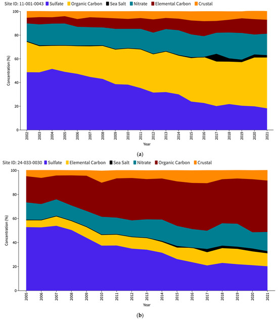
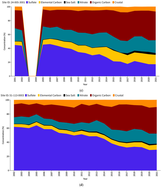
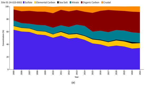
Figure 1.
PM2.5 speciation (in percentage) trend for DC (a), Beltsville (b) and Essex (c) CSN stations; Madison County (d) and Piney Run (e) IMPROVE stations as reported in the EPA Our Nation’s Air annual 2023 report.
The primary aim of this technical study is to explore the methodologies employed by the CSN for quantifying sea salt aerosols, emphasizing a pivotal methodological shift in 2017 and its implications. This research examines the SSA measurements gathered from various monitoring sites, assessing whether the notable increase in the reported SSA levels following 2017 is a long-term trend or a result of short-term variability. By analyzing the data collected over the past two decades, with a specific focus on sites in the BWC area, this paper seeks to determine whether the observed trends are restricted to the CSN network or are also present in other networks, such as IMPROVE. Additionally, it aims to investigate whether the sharp increase in SSA levels was caused by measurement or reporting errors.
2. Methodology
2.1. Network Description and Sampling
In the United States, two major networks play crucial roles in assessing PM2.5 speciation, providing critical insights into air quality dynamics—the Interagency Monitoring of Protected Visual Environments (IMPROVE) and the Chemical Speciation Network (CSN). Established in 1985, after the 1977 amendments to the Clean Air Act, IMPROVE monitors the air quality in national parks and wilderness areas, using modern equipment to evaluate particulate matter composition, and currently, there are approximately 160 active sites [12]. In reaction to the health-oriented National Ambient Air Quality Standards (NAAQS) for PM2.5 established in 1997, the CSN was established by the US EPA in 1997 to complement the National PM2.5 Monitoring Network (https://www.epa.gov/amtic/chemical-speciation-network-csn, accessed on 10 June 2024). This network comprises the Speciation Trends Network (STN) and supplemental speciation sites. Employment of CSN data has helped achieve various goals including the development of effective State Implementation Plans, formulation of emission control strategies, interpretation of health studies, and characterization of the spatial variation of aerosols throughout the year. In 2020, the CSN had around 50 STN sites and 100 State and Local Air Monitoring Stations (SLAMS) supplemental sites. The CSN program enhances the coverage of IMPROVE by adding monitoring sites in heavily populated urban areas [13,14].
Figure 2 shows the geographical distribution of IMPROVE (red dots) and CSN (blue dots) air quality monitoring networks in the mainland USA. IMPROVE sites are heavily concentrated in the western states, particularly in natural and protected areas such as the national parks, aligning with their focus on visibility and air quality in these regions. In contrast, CSN sites are more evenly distributed but denser in Eastern USA, particularly in the Midwest, Northeast, and along the Atlantic coast, targeting urban and suburban areas to analyze PM pollution.
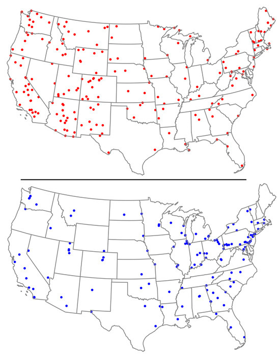
Figure 2.
Location of IMPROVE sites (red dots, top) and CSN sites (blue dots, bottom) throughout mainland USA. Source: Federal Land Manager Environmental Database.
Since 2000, CSN and the IMPROVE network have followed a similar sampling process where samples are collected every three days from the monitoring sites. However, the sampling process involves independent sampling techniques and specific filter media. The CSN and IMPROVE networks focus on measuring various components present in the air, including major anions, carbonaceous material, and a range of trace elements. In addition to measuring major anions and carbonaceous material, the CSN network directly measures ammonium (NH4+) and other cations. On the other hand, the IMPROVE network estimates ammonium levels by assuming that the measured sulfate (SO42−) and nitrate ions (NO3−) are completely neutralized. The IMPROVE network also measures chloride and nitrite (NO2−) ions from the beginning of its operations [12]. The data samples at both the sites are systematically gathered according to a 1-in-3 sampling schedule, wherein an integrated 24 h sample is collected every third day.
While the CSN and IMPROVE networks share similarities in their field and laboratory approaches, several subtle differences exist in their sampling and chemical analysis methods. These differences include variations in the techniques used to collect samples and analyze the chemical composition of the collected samples. For this study, the focus is on the measurement of chlorine and chloride. Both the CSN and IMPROVE networks use specific methods for these measurements. They utilize energy dispersive X-ray fluorescence (EDXRF) to measure the chlorine levels, and nylon ion chromatography to measure the chloride levels. There are differences in the acceptance testing protocols between IMPROVE and the CSN, but the impact on measurements is likely minimal due to the rigorous approach of collecting and analyzing blanks throughout the sampling and analysis process [14]. Blanks are used as controls to identify and quantify any contamination or artifacts introduced during collection, processing, transportation, and analysis, thereby improving the data’s reliability and validity [15]. Over time, the CSN’s methodologies have become more like those of IMPROVE [16,17]. Starting with samples obtained in November 2015, a new contractor was hired to analyze and report on the CSN data.
2.2. Sea Salt Aerosol Calculation from Tracers
Accurately quantifying the contribution of sea salt aerosol to the total mass of PM2.5 is crucial for understanding the composition and sources of atmospheric PM. To achieve this, the identification and utilization of appropriate tracers/markers play a pivotal role. Among the numerous constituents of sea salt, sodium and chlorine emerge as the prominent tracers due to their prevalence and distinctive analytical signatures. In the literature, it is assumed that other significant sources of Na and Cl in the atmosphere are negligible, and hence their concentrations can be employed to estimate the concentration of freshly formed sea salt particles in the air. This estimation relies on the relative contribution of Na and Cl in sea salt (Table 1), as determined by the work of [7]. By dividing the concentration of Na or Cl by their respective relative contributions, the concentration of sea salt particles is derived.

Table 1.
Mass contribution (g/g) of selected elements in fresh sea salt (Millero, 2006).
The computation of sea salt concentrations follows a simple relationship—the concentration of sea salt particles (in μg/m3) equals the reciprocal of the element’s mass fraction in sea water multiplied by the concentration of the tracer. For chlorine, the sea salt particle concentration is given by 1 divided by 0.554, multiplied by the Cl concentration, which yields a factor of 1.8 times the Cl concentration. Similarly, for Na, the sea salt particle concentration is obtained by dividing 1 by 0.308, and then multiplying it by the Na concentration, resulting in a factor of 3.26 times the Na concentration. This calculation is also based on the major and minor constituents of seawater and marine aerosols described in detail by [18]. The EPA, following the research conducted by [6], calculates sea salt concentrations as 1.8 times the chloride measurement when available, or alternatively, 1.8 times the chlorine measurement.
2.3. Study Area
The Baltimore–Washington Corridor (BWC) was chosen as the research region due to its vital relevance in terms of air quality and strategic position. The BWC is a major metropolitan center in the Mid-Atlantic region of the United States, spanning the urban and suburban areas between Baltimore, Maryland, and Washington, D.C. It is particularly sensitive to many air contaminants, owing to its geographical location and high degree of urbanization [19]. The area has significant air quality concerns due to mobility emissions, industrial activity, and its geographic location. The BWC, which is home to several manufacturing factories, power stations, and other industrial facilities, emits considerable amounts of pollutants into the atmosphere, including SO2, nitrogen oxides (NOx = NO + NO2), and particulate matter (PM) [20].
The BWC has three prominent air monitoring sites in the BWC region, namely McMillan NCore-PAMS (DC), HU-Beltsville (Beltsville) and Essex (Essex), all of which belong to the CSN. These stations play a crucial role in collecting data that reflect the cumulative impact of emissions, particularly near industrial sources (Figure 3). Multiple CSN stations in the region ensure detailed chemical analyses of PM, helping to identify pollution trends and sources and aiding in developing strategies to improve air quality.
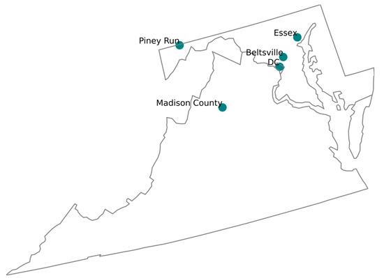
Figure 3.
Location of the DC, Beltsville, and Essex (as part of CSN); Madison County and Piney Run (as part of IMPROVE).
To conduct a fair and insightful analysis of the PM speciation dataset trend from the BWC CSN, we chose the two nearest IMPROVE stations, namely Madison County, Virginia, and Piney Run, Maryland (Figure 3). This allowed for a thorough review of the long-term datasets from each station, allowing for the detection and explanation of any SSA measurement/calculation anomalies that may exist. The authors recognize that these stations, part of different networks, are situated in varying environmental conditions, which may influence the measurement of SSA concentrations. Despite potential variations, the study primarily focused on the overarching long-term trends in the SSA concentration levels. By examining the PM speciation dataset acquired over time, we aimed to gain a comprehensive understanding of regional air quality trends, with a special emphasis on SSAs.
3. Results
3.1. Sea Salt Aerosol Trend
3.1.1. Percentage of SSAs in the Total PM2.5 Speciation
Table 2 provides a comprehensive overview of the relative contribution of sea salt aerosols to the total PM2.5 concentration at the study sites, as seen in Figure 1 as well. Analysis of the data from the CSN sites spanning from 2005 to 2014 shows that sea salt particles constitute the smallest fraction of PM2.5 compared to other constituents such as crustal matter, organic carbon, elemental carbon, nitrate, and sulfate, whereas in case of the IMPROVE sites, the slight increase in SSA percentage can be observed starting from 2011. This finding suggests that within the specified period, SSAs had a relatively minor influence on the overall PM2.5 concentration levels in the study region. The average percentage of SSA during this period was recorded as 0.43%, 0.35%, and 0.56% at the DC, Beltsville, and Essex monitoring stations, respectively. However, an intriguing shift in sea salt aerosol levels emerged in 2015, as evidenced by a substantial increase in its proportion. Remarkably, the Beltsville station stands out with a particularly high percentage of SSAs, approximately three times greater than its average during 2005–2014. In contrast, the DC and Essex stations exhibit comparatively lower percentage increases during the same period.
Table 2.
Percentage of sea salt aerosol in the total PM2.5 speciation measured at the study sites [21].
In 2016, a notable decline was observed across all three stations, with SSAs contributing to the lowest proportion of PM2.5 during that year. However, this downturn is short-lived, as a significant upsurge occurred in 2017 for all three CSN sites, with DC showing a significant increase to 6.5% from just 0.1% the previous year. Following the spike in 2017, each of the three CSN locations experienced a decline in subsequent years, although the percentages remained higher than the pre-2017 levels. The two IMPROVE sites, while also showing an increase in 2011, did not exhibit sharp peaks as the CSN sites did. Madison County showed a higher baseline from 2011 onwards, with its peak occurring in 2020 (1.8%). Piney Run’s data are generally the lowest of all the sites but follows the overall trend of a slight increase in 2011 onwards. Thus, the comparison between the CSN and IMPROVE dataset trends highlights a striking divergence in the SSA percentages. The data suggest that the CSN sites registered notably higher SSA levels from 2017 onwards.
3.1.2. Annual Average of SSA Concentrations
Figure 4 presents a comprehensive analysis of the annual average sea salt trends in the study area from 2001 to 2021. Notably, the absence of data for the Essex site in 2003 and 2004 contributes to a discontinuity in the trend. Madison county has data available from 2004, whereas the Beltsville and Piney Run sites provide data from 2005 onwards. This discrepancy in data availability also underscores the importance of continuous monitoring to maintain a comprehensive understanding of the PM2.5 speciation trends.
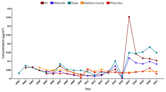
Figure 4.
Two decades of SSA trend in the study area from 2001 to 2021, showing the annual average concentrations.
Examining the measured sea salt levels over time, a slight increase was observed in 2007 at both the DC and Essex sites, although the trend declined until 2012. During this time, Essex regularly had slightly elevated annual average SSA concentrations than DC, an observation that could be attributed to the Essex site’s proximity to the Baltimore Bay region. In contrast, the Beltsville site reported lower annual average SSA concentrations, most likely due to its location, which is further away from coastal area. From 2013, a consistent trend appeared as all three CSN sites showed a progressive increase in SSA levels, which lasted until 2015. In contrast to this ascending pattern, 2016 marked an unexpected decline in the SSA levels throughout these CSN sites. This shift cannot be attributed to missing measurements or datasets. From 2017, the data show a pronounced surge in SSA levels, notably at the DC location, which witnessed the most significant escalation in the same year. This major increase only being recorded in the DC site, unlike the moderate trends at Beltsville and Essex, suggests no shared large-scale event or change in environmental conditions of the BWC. Madison county generally showed a stable or slight downward trend with a small noticeable peak in 2004 and 2011. Piney Run exhibited a relatively stable trend with minor fluctuations in 2011 and 2020. The increase in SSA levels from 2010 to 2011 for both these IMPROVE sites is minor as compared to the one measured by the CSN sites between 2016 and 2017.
The consistently moderate concentrations of SSA observed at the IMPROVE sites suggest that the SSAs may be attenuated due to transport and aging, given that these sites are located a long distance from the coastal areas where such particles originate. The decrease in SSA levels is likely attributed to the deposition and dispersion processes that occur when aerosols move inland. However, the disparity becomes more evident when we look at the CSN sites. Despite being impacted by regional emissions from various sources—industrial operations, urban emissions, or natural contributions from the surrounding environment—the CSN sites showed increased SSA concentrations, notably after 2016. This significant increase raises concerns, implying potential technological or procedural changes within the monitoring system that went into force around 2017. These modifications might account for the observed increase in reported levels, indicating improvements in detection capabilities or updates to monitoring techniques that resulted in a more accurate depiction of the SSA abundance in these places.
3.2. Domination of Chloride over Chlorine Measurements
Figure 5 displays the measurements of chlorine and chloride taken at the Essex site during the study period. All three CSN sites display similar trends, and hence Essex is used as a representative of the other two sites. The concentration of chlorine remained relatively low throughout the period, with no significant changes occurring during or after 2017. This trend suggests a consistent and stable presence of chlorine at the site. On the contrary, the chloride levels measured at the station were consistently higher since the commencement of the measurements. We observed continuous and relatively higher concentrations of chloride compared to chlorine. The annual average sea salt concentrations from 2017 to 2021, presented in Table 3, support this observation. The data reveal that the annual average chloride concentration is approximately ten times greater than the annual average chlorine concentration, indicating a significant disparity between the two.
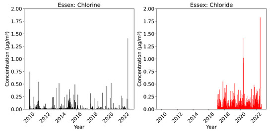
Figure 5.
Bar representation of chlorine (black) and chloride (red) measurements at the Essex.
Table 3.
Comparisons between annual average of chlorine and chloride data from the Essex CSN station from 2017 to 2021.
Interestingly, similar patterns were also noted at the other two sites in the BWC, suggesting that the lower chlorine levels are not specific to the Essex site alone but may be a characteristic of the entire region. The lower chlorine levels could be attributed to its depletion through atmospheric chemical reactions, leading to its conversion or loss into the gas phase. These reactions can occur between chlorine and various compounds present in the atmosphere [22]. Consequently, the chlorine concentration at the site remains consistently low.
The CSN began reporting chloride concentrations in February 2017, marking a pivotal methodological shift with substantial implications for the way SSA was calculated. The use of chloride as a marker for SSA measurement was a change from the previous usage of chlorine for the same purpose. This transition was crucial in interpreting the SSA data trends, as chloride tends to be present in higher concentrations and is a more substantial constituent of sea salt compared to elemental chlorine. As a result of this analytical refinement, the CSN stations began reporting higher SSA concentrations from 2017 onwards. This methodological change explains the significant increase in SSA percentages recorded after 2017 by the CSN sites, a trend that deviates sharply from the traditionally lower percentages.
Table 4 presents a comprehensive analysis of the data for chlorine and chloride measured at Essex CSN over a span of five years, from 2017 to 2021. The data includes key statistical measures such as the mean, standard deviation, standard error of the mean, and coefficient of variation (%), which are crucial for understanding the behavior and trends of these chemical elements. Chloride has a significantly higher mean compared to chlorine, indicating that, on average, the chloride measurements are higher than the chlorine measurements. During the study period, chloride also exhibited a larger standard deviation compared to chlorine, indicating that the measurements of chloride vary more widely around their mean than the measurements of chlorine do around their mean. However, chlorine measurements displayed a higher coefficient of variation compared to chloride. This indicates that the measurements of chlorine exhibit significantly more variability around their mean than the measurements of chloride.
Table 4.
Essential statistical measures such as mean, standard deviation, standard error of mean and coefficient of variation (%) for chlorine and chloride measurements from Essex CSN site from 2017 to 2021.
4. Conclusions and Discussions
The EPA, following the research conducted in 2008, calculates SSA concentrations as 1.8 times the chloride measurement when available, or alternatively, 1.8 times the chlorine measurement [6]. The 1.8 factor accounts for the other sea salt components like sodium, which is directly measured by the network’s routine analyses [7]. However, the observations show significantly lower measured chlorine concentrations at the speciation sites compared to chloride concentrations. If chloride is considered a more accurate tracer for SSA instead of chlorine, then the calculation of SSA performed prior to 2017 using chlorine values by the CSN would show systematically lower concentrations. This discrepancy highlights the potential for erroneous reporting of SSA concentrations if chlorine is used as the only tracer for SSA measurement. Also, this methodological oversight could have led to significant underestimations of SSA levels in previous analyses, impacting the accuracy and reliability of air quality assessments. Consequently, this finding should be taken into consideration when estimating SSA concentrations at sites where the chloride levels are not reported. The disparity between the recorded chlorine and chloride concentrations at CSN locations in the study area (BWC) makes a strong case for a more sophisticated method to determine sea salt aerosol levels. While the EPA has historically used a factor of 1.8 times the chloride value, or 1.8 times the chlorine measurement, this study underscores the need for a more rigorous technique. Given the observed discrepancies in chlorine and chloride concentrations, a single tracer may not adequately represent sea salt aerosol levels. Hence, we recommend the use of more than one tracer for extensive verification of sea salt aerosol amounts. Beyond the traditional use of chlorine or chloride alone, including an extra tracer might improve computation accuracy. This method would require cross-referencing readings from two separate tracers, resulting in a more reliable and representative estimate of sea salt aerosol concentrations. Pairing chlorine or chloride with another compound that exhibits a distinct response to sea salt aerosol could better account for variations in sea salt composition and improve the precision of concentration estimates.
The analysis of the dataset from the Essex CSN site revealed notable trends and patterns in chlorine and chloride concentrations over the five-year study period. The chlorine concentrations displayed considerable fluctuations, as evidenced by the high coefficient of variation (%). This indicates that chlorine levels were subject to seasonal or episodic changes during the study period, indicating potential local environmental forcing factors. In contrast, the chloride concentrations exhibited more stable trends, as reflected by a lower coefficient of variation (%). The calculated standard errors of the means estimated for both chlorine and chloride provided a reliable basis for the annual mean values, contributing to the robustness of the results. The observed fluctuations in chlorine concentrations emphasize the need for continuous monitoring and assessment of potential sources of contamination.
The findings presented in this study have significant implications for the policymakers and stakeholders involved in assessing and managing air quality at the state and national levels for more accurate future assessments. Policymakers rely on accurate and reliable data to make informed decisions regarding air quality regulations, public health measures, and environmental protection strategies. The subtle variations in data collection and reporting, specifically in relation to sea salt aerosol levels (which are calculated by measuring its tracers), underscore the need for harmonization and standardization across monitoring networks. This is particularly crucial when interpreting historical data or conducting comparative analyses between different monitoring sites or regions. Strong differences in calculated sea salt aerosol concentrations, based on differences in chloride and chlorine measurements, highlight the importance of reconsidering the current calculation methodologies.
We also recommend that the data reporting agency adopt the term ‘salt’ rather than ‘sea salt’ when specifying this particular PM2.5 speciation. This adjustment is crucial for a more comprehensive representation of the particles’ sources. Using the term ‘sea salt’ inherently limits the understanding of the particle’s origin to ocean spray, thereby excluding other significant sources such as dry lakebeds, chemical industries, and other anthropogenic activities. By using the broader term ‘salt’, we ensure that both natural and anthropogenic sources are adequately covered. This change will enhance the accuracy of data reporting and analysis, leading to better-informed environmental policies and research outcomes. Accurate terminology is essential for precise data interpretation and adopting ‘salt’ will contribute to a more holistic understanding of particulate matter in various environmental contexts.
Author Contributions
The conceptualization was performed by N.N.K. and R.K.S.; N.N.K. and R.K.S. curated the data. The methodology and investigation were completed by N.N.K.; N.N.K., R.K.S., S.C., R.M.F. and W.R.S. performed the analysis. N.N.K. drafted the original paper, which was reviewed and edited by R.K.S., R.M.F. and W.R.S.; S.C. contributed significantly to improving this work. Supervision was the responsibility of R.K.S. and S.C. All authors have read and agreed to the published version of the manuscript.
Funding
This research is based on work supported by the U.S. Department of Commerce, National Oceanic and Atmospheric Administration, Educational Partnership Program under Agreement No. NA22SEC4810015.
Data Availability Statement
The data supporting the findings of this study are accessible from the US Environmental Protection Agency. Air Quality System Data Mart [internet database] available at http://www.epa.gov/ttn/airs/aqsdatamart, accessed on 10 June 2024.
Acknowledgments
Authors want to thank staff at the Environmental Protection Agency (EPA) Datamart and Maryland Department of Environment (MDE) for their cooperation in this study. IMPROVE is a collaborative association of state, tribal, and federal agencies, and international partners. The US Environmental Protection Agency is the primary funding source, with contracting and research support from the National Park Service. The Air Quality Group at the University of California, Davis, is the central analytical laboratory, with ion analysis provided by Research Triangle Institute, and carbon analysis provided by Desert Research Institute.
Conflicts of Interest
The authors declare no conflicts of interest. The funders had no role in the design of the study; in the collection, analyses, or interpretation of data; in the writing of the manuscript; or in the decision to publish the results.
References
- Seinfeld, J.H.; Pandis, S.N. Atmospheric Chemistry and Physics: From Air Pollution to Climate Change; John Wiley Sons: Hoboken, NJ, USA, 2016; p. 49. [Google Scholar]
- Crawford, J.; Cohen, D.D.; Chambers, S.D.; Williams, A.G.; Atanacio, A. Impact of aerosols of sea salt origin in a coastal basin: Sydney, Australia. Atmos. Environ. 2019, 207, 52–62. [Google Scholar] [CrossRef]
- Feng, L.; Shen, H.; Zhu, Y.; Gao, H.; Yao, X. Insight into generation and evolution of sea-salt aerosols from field measurements in diversified marine and coastal atmospheres. Sci. Rep. 2017, 7, 41260. [Google Scholar] [CrossRef] [PubMed]
- Quinn, P.; Miller, T.; Bates, T.; Ogren, J.; Andrews, E.; Shaw, G. A 3-year record of simultaneously measured aerosol chemical and optical properties at Barrow, Alaska. J. Geophys. Res. Atmos. 2002, 107, AAC–8. [Google Scholar] [CrossRef]
- Nakajima, T.; Higurashi, A.; Kawamoto, K.; Penner, J.E. A possible correlation between satellite-derived cloud and aerosol microphysical parameters. Geophys. Res. Lett. 2001, 28, 1171–1174. [Google Scholar] [CrossRef]
- White, W.H. Chemical markers for sea salt in IMPROVE aerosol data. Atmos. Environ. 2008, 42, 261–274. [Google Scholar] [CrossRef]
- Millero, F. Physicochemical Controls. Ocean. Mar. Geochem. 2006, 6, 1. [Google Scholar]
- Pakkanen, T.A. Study of formation of coarse particle nitrate aerosol. Atmos. Environ. 1996, 30, 2475–2482. [Google Scholar] [CrossRef]
- Bertram, T.H.; Cochran, R.E.; Grassian, V.H.; Stone, E.A. Sea spray aerosol chemical composition: Elemental and molecular mimics for laboratory studies of heterogeneous and multiphase reactions. Chem. Soc. Rev. 2018, 47, 2374–2400. [Google Scholar] [CrossRef] [PubMed]
- Keene, W.C.; Pszenny, A.A.; Jacob, D.J.; Duce, R.A.; Galloway, J.N.; Schultz-Tokos, J.J.; Sievering, H.; Boatman, J.F. The geochemical cycling of reactive chlorine through the marine troposphere. Glob. Biogeochem. Cycles 1990, 4, 407–430. [Google Scholar] [CrossRef]
- Hopkins, R.J.; Desyaterik, Y.; Tivanski, A.V.; Zaveri, R.A.; Berkowitz, C.M.; Tyliszczak, T.; Gilles, M.K.; Laskin, A. Chemical speciation of sulfur in marine cloud droplets and particles: Analysis of individual particles from the marine boundary layer over the California current. J. Geophys. Res. Atmos. 2008, 113, D04209. [Google Scholar] [CrossRef]
- Malm, W.C.; Schichtel, B.A.; Pitchford, M.L.; Ashbaugh, L.L.; Eldred, R.A. Spatial and monthly trends in speciated fine particle concentration in the United States. J. Geophys. Res. Atmos. 2004, 109, 1–22. [Google Scholar] [CrossRef]
- Flanagan, J.B.; Jayanty, R.K.; Rickman, E.E., Jr.; Peterson, M.R. PM2. 5 Speciation Trends Network: Evaluation of whole-system uncertainties using data from sites with collocated samplers. J. Air Waste Manag. Assoc. 2006, 56, 492–499. [Google Scholar] [CrossRef][Green Version]
- Solomon, P.A.; Crumpler, D.; Flanagan, J.B.; Jayanty, R.; Rickman, E.E.; McDade, C.E. US national PM2. 5 chemical speciation monitoring networks—CSN and IMPROVE: Description of networks. J. Air Waste Manag. Assoc. 2014, 64, 1410–1438. [Google Scholar] [CrossRef]
- Chow, J.C.; Watson, J.G.; Chen, L.W.; Rice, J.; Frank, N.H. Quantification of PM 2.5 organic carbon sampling artifacts in US networks. Atmos. Chem. Phys. 2010, 10, 5223–5239. [Google Scholar] [CrossRef]
- Gutknecht, W.; Flanagan, J.; McWilliams, A.; Jayanty, R.K.; Kellogg, R.; Rice, J.; Duda, P.; Sarver, R.H. Harmonization of uncertainties of X-ray fluorescence data for PM2. 5 air filter analysis. J. Air Waste Manag. Assoc. 2010, 60, 184–194. [Google Scholar] [CrossRef] [PubMed]
- Spada, N.J.; Hyslop, N.P. Comparison of elemental and organic carbon measurements between IMPROVE and CSN before and after method transitions. Atmos. Environ. 2018, 178, 173–180. [Google Scholar] [CrossRef]
- Warneck, P. Chemistry of the Natural Atmosphere; Elsevier: Amsterdam, The Netherlands, 1999; Volume 71. [Google Scholar]
- Chen, L.W.A.; Doddridge, B.G.; Dickerson, R.R.; Chow, J.C.; Henry, R.C. Origins of fine aerosol mass in the Baltimore–Washington corridor: Implications from observation, factor analysis, and ensemble air parcel back trajectories. Atmos. Environ. 2002, 36, 4541–4554. [Google Scholar] [CrossRef]
- Dreessen, J.; Ren, X.; Gardner, D.; Green, K.; Stratton, P.; Sullivan, J.T.; Delgado, R.; Dickerson, R.R.; Woodman, M.; Berkoff, T.; et al. VOC and trace gas measurements and ozone chemistry over the Chesapeake Bay during OWLETS-2, 2018. J. Air Waste Manag. Assoc. 2023, 73, 178–199. [Google Scholar] [CrossRef] [PubMed]
- US Environmental Protection Agency. Air Quality System Data Mart. Available online: https://www.epa.gov/ttn/airs/aqsdatamart (accessed on 30 March 2024).
- Calvert, J.G.; Orlando, J.J.; Stockwell, W.R.; Wallington, T.J. The Mechanisms of Reactions Influencing Atmospheric Ozone; Oxford University Press: Oxford, UK, 2015. [Google Scholar]


Disclaimer/Publisher’s Note: The statements, opinions and data contained in all publications are solely those of the individual author(s) and contributor(s) and not of MDPI and/or the editor(s). MDPI and/or the editor(s) disclaim responsibility for any injury to people or property resulting from any ideas, methods, instructions or products referred to in the content. |
© 2024 by the authors. Licensee MDPI, Basel, Switzerland. This article is an open access article distributed under the terms and conditions of the Creative Commons Attribution (CC BY) license (https://creativecommons.org/licenses/by/4.0/).