
Comparison of Future Design Rainfall with Current Design Rainfall: A Case Study in New South Wales, Australia


Abstract
1. Introduction
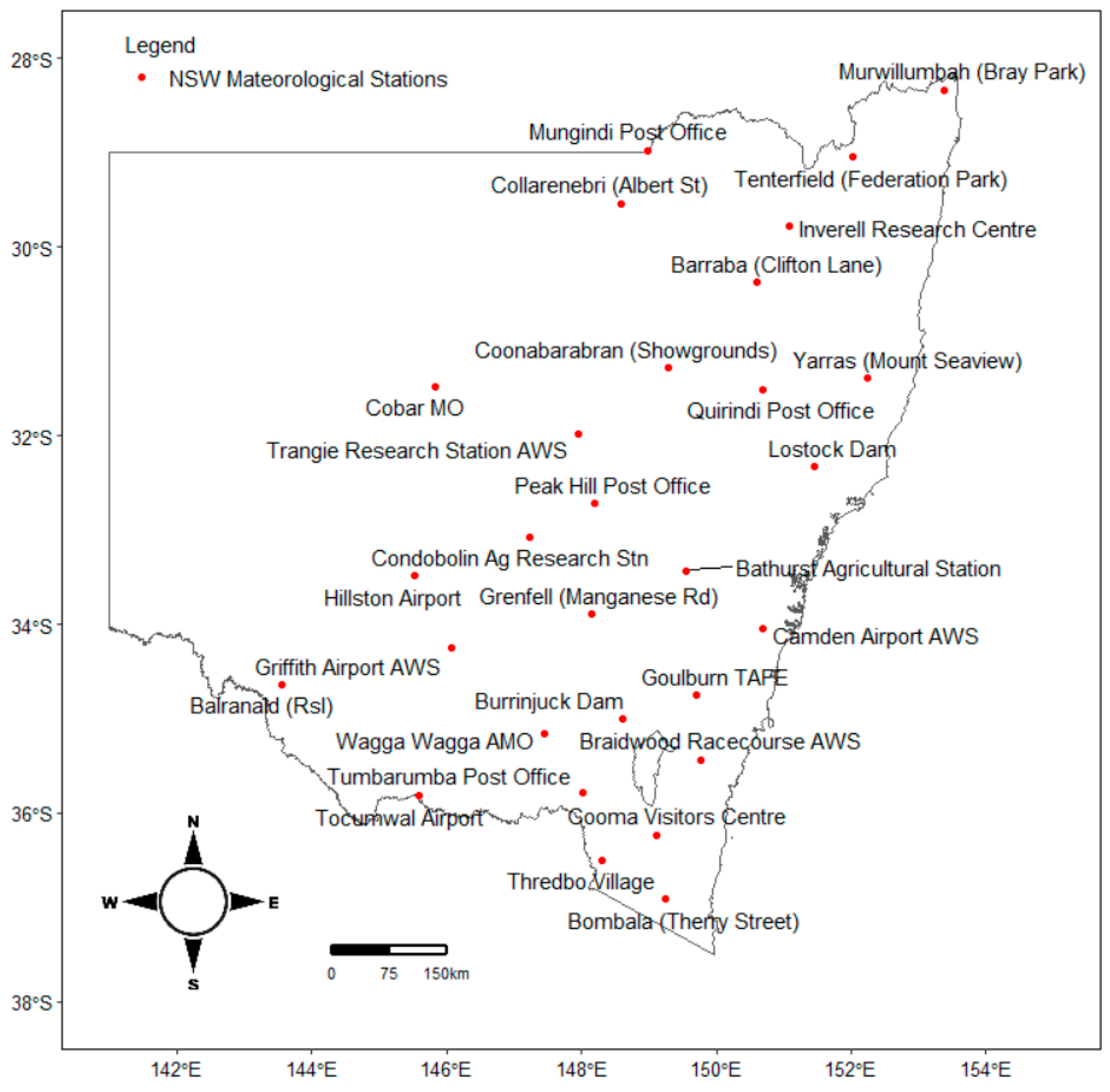
2. Study Area
Rainfall Data
3. Methods
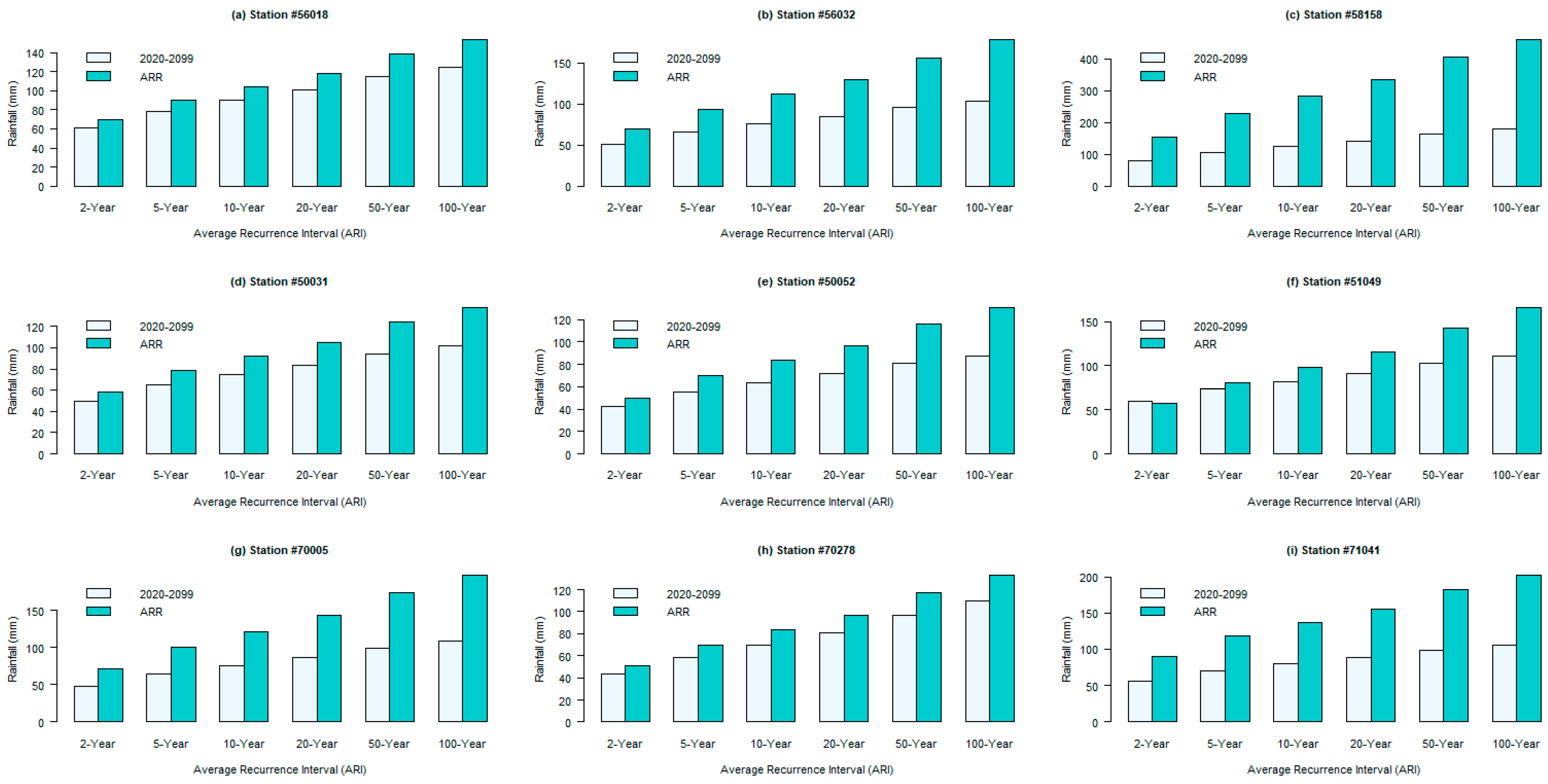
4. Results and Discussion
5. Conclusions and Recommendations
- Future extreme rainfall will be significantly impacted by climate change in most parts of NSW; nevertheless, this change has different impacts on different recurrence intervals.
- The future design rainfall will be decreased in most of the locations in NSW, indicating the potential for drought with the changing climate.
- The probability of the occurrence of an increase in the future design rainfall is 4.7%, whereas the probability of a decrease in the design rainfall is up to 60% for the 100-year recurrence interval. This changing rate varies amongst the recurrence intervals. However, the design rainfall will decrease for most of the meteorological stations in NSW.
- Stormwater management infrastructure that is designed from historical extreme rainfall will lead to over-design or under-design, leading to uncertainty in flood mitigation. Global climate model and return periods have considerable influence on the extent of this uncertainty.
Author Contributions
Funding
Institutional Review Board Statement
Informed Consent Statement
Data Availability Statement
Conflicts of Interest
References
- Hettiarachchi, S.; Wasko, C.; Sharma, A. Increase in flood risk resulting from climate change in a developed urban watershed–the role of storm temporal patterns. Hydrol. Earth Syst. Sci. 2018, 22, 2041–2056. [Google Scholar] [CrossRef]
- Yilmaz, A.G.; Perera, B.J.C. Extreme Rainfall Nonstationarity Investigation and Intensity–Frequency–Duration Relationship. J. Hydrol. Eng. 2014, 19, 1160–1172. [Google Scholar] [CrossRef]
- Fadhel, S.; Rico-Ramirez, M.A.; Han, D. Uncertainty of intensity–duration–frequency (IDF) curves due to varied climate baseline periods. J. Hydrol. 2017, 547, 600–612. [Google Scholar] [CrossRef]
- Myhre, G.; Alterskjær, K.; Stjern, C.W.; Hodnebrog, Ø.; Marelle, L.; Samset, B.H.; Sillmann, J.; Schaller, N.; Fischer, E.; Schulz, M. Frequency of extreme precipitation increases extensively with event rareness under global warming. Sci. Rep. 2019, 9, 16063. [Google Scholar] [CrossRef] [PubMed]
- Boylan, S.; Beyer, K.; Schlosberg, D.; Mortimer, A.; Hime, N.; Scalley, B.; Alders, R.; Corvalan, C.; Capon, A. A conceptual framework for climate change, health and wellbeing in NSW, Australia. Public Health Res. Pract. 2018, 28, e2841826. [Google Scholar] [CrossRef] [PubMed]
- Mirhosseini, G.; Srivastava, P.; Stefanova, L. The impact of climate change on rainfall Intensity–Duration–Frequency (IDF) curves in Alabama. Reg. Environ. Change 2013, 13, 25–33. [Google Scholar] [CrossRef]
- Yilmaz, A.G.; Hossain, I.; Perera, B.J.C. Effect of climate change and variability on extreme rainfall intensity–frequency–duration relationships: A case study of Melbourne. Hydrol. Earth Syst. Sci. 2014, 18, 4065–4076. [Google Scholar] [CrossRef]
- Abu Arra, A.; Şişman, E. Characteristics of hydrological and meteorological drought based on intensity-duration-frequency (IDF) curves. Water 2023, 15, 3142. [Google Scholar] [CrossRef]
- Bibi, T.S.; Tekesa, N.W. Impacts of climate change on IDF curves for urban stormwater management systems design: The case of Dodola Town, Ethiopia. Environ. Monit. Assess. 2023, 195, 170. [Google Scholar] [CrossRef]
- Tousi, E.G.; O’Brien, W.; Doulabian, S.; Toosi, A.S. Climate changes impact on stormwater infrastructure design in Tucson Arizona. Sustain. Cities Soc. 2021, 72, 103014. [Google Scholar] [CrossRef]
- Bulti, D.T.; Abebe, B.G.; Biru, Z. Climate change–induced variations in future extreme precipitation intensity–duration–frequency in flood-prone city of Adama, central Ethiopia. Environ. Monit. Assess. 2021, 193, 784. [Google Scholar] [CrossRef] [PubMed]
- Butcher, J.B.; Zi, T.; Pickard, B.R.; Job, S.C.; Johnson, T.E.; Groza, B.A. Efficient statistical approach to develop intensity-duration-frequency curves for precipitation and runoff under future climate. Clim. Change 2021, 164, 3. [Google Scholar] [CrossRef] [PubMed]
- Cook, L.M.; McGinnis, S.; Samaras, C. The effect of modeling choices on updating intensity-duration-frequency curves and stormwater infrastructure designs for climate change. Clim. Change 2020, 159, 289–308. [Google Scholar] [CrossRef]
- Rosenberg, E.A.; Keys, P.W.; Booth, D.B.; Hartley, D.; Burkey, J.; Steinemann, A.C.; Lettenmaier, D.P. Precipitation extremes and the impacts of climate change on stormwater infrastructure in Washington State. Clim. Change 2010, 102, 319–349. [Google Scholar] [CrossRef]
- Kourtis, I.M.; Tsihrintzis, V.A. Update of intensity-duration-frequency (IDF) curves under climate change: A review. Water Supply 2022, 22, 4951–4974. [Google Scholar] [CrossRef]
- Fowler, H.J.; Wasko, C.; Prein, A.F. Intensification of short-duration rainfall extremes and implications for flood risk: Current state of the art and future directions. Philos. Trans. R. Soc. A 2021, 379, 20190541. [Google Scholar] [CrossRef] [PubMed]
- Liang, C.; Li, D.; Yuan, Z.; Liao, Y.; Nie, X.; Huang, B.; Wu, X.; Xie, Z. Assessing urban flood and drought risks under climate change, China. Hydrol. Process. 2019, 33, 1349–1361. [Google Scholar] [CrossRef]
- Yilmaz, A.G.; Perera, B.J.C. Spatiotemporal Trend Analysis of Extreme Rainfall Events in Victoria, Australia. Water Resour. Manag. 2015, 29, 4465–4480. [Google Scholar] [CrossRef]
- Herath, S.M.; Sarukkalige, R.; Nguyen, V.T.V. Evaluation of empirical relationships between extreme rainfall and daily maximum temperature in Australia. J. Hydrol. 2018, 556, 1171–1181. [Google Scholar] [CrossRef]
- Hajani, E.; Rahman, A.; Ishak, E. Trends in extreme rainfall in the state of New South Wales, Australia. Hydrol. Sci. J. 2017, 62, 2160–2174. [Google Scholar] [CrossRef]
- Hossain, I.; Esha, R.; Alam Imteaz, M. An Attempt to Use Non-Linear Regression Modelling Technique in Long-Term Seasonal Rainfall Forecasting for Australian Capital Territory. Geosciences 2018, 8, 282. [Google Scholar] [CrossRef]
- Hossain, I.; Rasel, H.M.; Imteaz, M.A.; Mekanik, F. Long-term seasonal rainfall forecasting: Efficiency of linear modelling technique. Environ. Earth Sci. 2018, 77, 280. [Google Scholar] [CrossRef]
- Hossain, I.; Rasel, H.M.; Imteaz, M.A.; Mekanik, F. Long-term seasonal rainfall forecasting using linear and non-linear modelling approaches: A case study for Western Australia. Meteorol. Atmos. Phys. 2020, 132, 331–341. [Google Scholar] [CrossRef]
- Khastagir, A.; Hossain, I.; Anwar, A.H.M.F. Efficacy of linear multiple regression and artificial neural network for long-term rainfall forecasting in Western Australia. Meteorol. Atmos. Phys. 2022, 134, 69. [Google Scholar] [CrossRef]
- CSIRO; Australian Bureau of Meteorology. State of the Climate 2020. Available online: http://www.bom.gov.au/state-of-the-climate/2020/ (accessed on 1 November 2021).
- Olson, R.; Evans, J.P.; Di Luca, A.; Argüeso, D. The NARCliM project: Model agreement and significance of climate projections. Clim. Res. 2016, 69, 209–227. [Google Scholar] [CrossRef]
- Yazdanfar, Z.; Sharma, A. Urban drainage system planning and design–challenges with climate change and urbanization: A review. Water Sci. Technol. 2015, 72, 165–179. [Google Scholar] [CrossRef]
- Martel, J.-L.; Brissette, F.P.; Lucas-Picher, P.; Troin, M.; Arsenault, R. Climate change and rainfall intensity-duration-frequency curves: Overview of science and guidelines for adaptation. J. Hydrol. Eng. 2021, 26, 03121001. [Google Scholar] [CrossRef]
- Meresa, H.; Tischbein, B.; Mekonnen, T. Climate change impact on extreme precipitation and peak flood magnitude and frequency: Observations from CMIP6 and hydrological models. Nat. Hazards 2022, 111, 2649–2679. [Google Scholar] [CrossRef]
- Hajani, E. Climate change and its influence on design rainfall at-site in New South Wales State, Australia. J. Water Clim. Change 2020, 11, 251–269. [Google Scholar] [CrossRef]
- Australian Bureau of Meteorology. 2022. Available online: http://www.bom.gov.au/climate/data/?ref=ftr (accessed on 1 November 2021).
- Doulabian, S.; Tousi, E.G.; Shadmehri Toosi, A.; Alaghmand, S. Non-stationary precipitation frequency estimates for resilient infrastructure design in a changing climate: A case study in Sydney. Hydrology 2023, 10, 117. [Google Scholar] [CrossRef]
- Wasko, C.; Guo, D.; Ho, M.; Nathan, R.; Vogel, E. Diverging projections for flood and rainfall frequency curves. J. Hydrol. 2023, 620, 129403. [Google Scholar] [CrossRef]
- Gu, H.; Yu, Z.; Wang, G.; Wang, J.; Ju, Q.; Yang, C.; Fan, C. Impact of climate change on hydrological extremes in the Yangtze River Basin, China. Stoch. Environ. Res. Risk Assess. 2015, 29, 693–707. [Google Scholar] [CrossRef]
- Sun, X.; Li, R.; Shan, X.; Xu, H.; Wang, J. Assessment of climate change impacts and urban flood management schemes in central Shanghai. Int. J. Disaster Risk Reduct. 2021, 65, 102563. [Google Scholar] [CrossRef]
- Smith, D.M.; Kniveton, D.R.; Barrett, E.C. A statistical modeling approach to passive microwave rainfall retrieval. J. Appl. Meteorol. Climatol. 1998, 37, 135–154. [Google Scholar] [CrossRef]
- ARC Centre of Excellence for Climate System Science. NSW and ACT Regional Climate Model (NARCliM) Project Dataset; ARC Centre of Excellence for Climate System Science: Sydney, Australia, 2012. [Google Scholar]
- Wi, S.; Valdés, J.B.; Steinschneider, S.; Kim, T.-W. Non-stationary frequency analysis of extreme precipitation in South Korea using peaks-over-threshold and annual maxima. Stoch. Environ. Res. Risk Assess. 2016, 30, 583–606. [Google Scholar] [CrossRef]
- Sane, Y.; Panthou, G.; Bodian, A.; Vischel, T.; Lebel, T.; Dacosta, H.; Quantin, G.; Wilcox, C.; Ndiaye, O.; Diongue-Niang, A. Intensity–duration–frequency (IDF) rainfall curves in Senegal. Nat. Hazards Earth Syst. Sci. 2018, 18, 1849–1866. [Google Scholar] [CrossRef]
- Anghel, C.G.; Ilinca, C. Predicting Future Flood Risks in the Face of Climate Change: A Frequency Analysis Perspective. Water 2023, 15, 3883. [Google Scholar] [CrossRef]
- Charras-Garrido, M.; Lezaud, P. Extreme Value Analysis: An Introduction. J. Société Française Stat. 2013, 154, 66–97. [Google Scholar]
- Hossain, I.; Imteaz, M.A.; Khastagir, A. Effects of estimation techniques on generalised extreme value distribution (GEVD) parameters and their spatio-temporal variations. Stoch. Environ. Res. Risk Assess. 2021, 35, 2303–2312. [Google Scholar] [CrossRef]
- Ilinca, C.; Anghel, C.G. Flood Frequency Analysis Using the Gamma Family Probability Distributions. Water 2023, 15, 1389. [Google Scholar] [CrossRef]
- Ilinca, C.; Anghel, C.G. Flood-Frequency Analysis for Dams in Romania. Water 2022, 14, 2884. [Google Scholar] [CrossRef]
- Khastagir, A.; Hossain, I.; Aktar, N. Evaluation of different parameter estimation techniques in extreme bushfire modelling for Victoria, Australia. Urban Clim. 2021, 37, 100862. [Google Scholar] [CrossRef]
- Feng, T.; Zhu, X.; Dong, W. Historical assessment and future projection of extreme precipitation in CMIP6 models: Global and continental. Int. J. Climatol. 2023, 43, 4119–4135. [Google Scholar] [CrossRef]
- Alam, M.S.; Elshorbagy, A. Quantification of the climate change-induced variations in Intensity–Duration–Frequency curves in the Canadian Prairies. J. Hydrol. 2015, 527, 990–1005. [Google Scholar] [CrossRef]
- DeGaetano, A.T.; Castellano, C.M. Future projections of extreme precipitation intensity-duration-frequency curves for climate adaptation planning in New York State. Clim. Serv. 2017, 5, 23–35. [Google Scholar] [CrossRef]
- Simonovic, S.P.; Peck, A. Updated Rainfall Intensity Duration Frequency Curves for the City of London under the Changing Climate; Department of Civil and Environmental Engineering, The University of Western: London, ON, Canada, 2009. [Google Scholar]
- Yang, L.; Franzke, C.L.E.; Duan, W. Evaluation and projections of extreme precipitation using a spatial extremes framework. Int. J. Climatol. 2023, 43, 3453–3475. [Google Scholar] [CrossRef]
- Hassan, W.H.; Nile, B.K.; Al-Masody, B.A. Climate change effect on storm drainage networks by storm water management model. Environ. Eng. Res. 2017, 22, 393–400. [Google Scholar] [CrossRef]
- Kundzewicz, Z.W.; Kanae, S.; Seneviratne, S.I.; Handmer, J.; Nicholls, N.; Peduzzi, P.; Mechler, R.; Bouwer, L.M.; Arnell, N.; Mach, K. Flood risk and climate change: Global and regional perspectives. Hydrol. Sci. J. 2014, 59, 1–28. [Google Scholar] [CrossRef]
- Nile, B.K.; Hassan, W.H.; Alshama, G.A. Analysis of the effect of climate change on rainfall intensity and expected flooding by using ANN and SWMM programs. ARPN J. Eng. Appl. Sci. 2019, 14, 974–984. [Google Scholar]
- Li, J.; Evans, J.; Johnson, F.; Sharma, A. A comparison of methods for estimating climate change impact on design rainfall using a high-resolution RCM. J. Hydrol. 2017, 547, 413–427. [Google Scholar] [CrossRef]


| Station No | Station Name | Latitude | Longitude | Elevation | Mean Extreme | Standard Deviation |
|---|---|---|---|---|---|---|
| 48027 | Cobar MO | 31.48 | 145.83 | 260 | 42.65 | 19.1 |
| 48031 | Collarenebri (Albert St) | 29.54 | 148.58 | 145 | 63.83 | 37.67 |
| 49002 | Balranald (Rsl) | 34.64 | 143.56 | 61 | 38.36 | 16.35 |
| 50031 | Peak Hill Post Office | 32.72 | 148.19 | 285 | 56.64 | 22.94 |
| 50052 | Condobolin Ag Research Stn | 33.07 | 147.23 | 195 | 43.20 | 17.94 |
| 51049 | Trangie Research Station AWS | 31.99 | 147.95 | 215 | 51.12 | 25.20 |
| 52020 | Mungindi Post Office | 28.98 | 148.99 | 160 | 61.04 | 25.67 |
| 54003 | Barraba (Clifton Lane) | 30.38 | 150.61 | 499 | 61.79 | 26.39 |
| 55049 | Quirindi Post Office | 31.51 | 150.68 | 390 | 57.61 | 18.53 |
| 56018 | Inverell Research Centre | 29.78 | 151.08 | 664 | 60.43 | 20.64 |
| 56032 | Tenterfield (Federation Park) | 29.05 | 152.02 | 838 | 66.41 | 26.66 |
| 58158 | Murwillumbah (Bray Park) | 28.34 | 153.38 | 8 | 147.3 | 67.68 |
| 60085 | Yarras (Mount Seaview) | 31.39 | 152.25 | 155 | 120.5 | 55.19 |
| 61288 | Lostock Dam | 32.33 | 151.46 | 200 | 69.78 | 33.47 |
| 63005 | Bathurst Agricultural Station | 33.43 | 149.56 | 713 | 49.09 | 17.62 |
| 64008 | Coonabarabran (Showgrounds) | 31.28 | 149.28 | 520 | 71.08 | 27.33 |
| 68192 | Camden Airport AWS | 34.04 | 150.69 | 74 | 78.30 | 36.94 |
| 69132 | Braidwood Racecourse AWS | 35.43 | 149.78 | 665 | 70.05 | 29.15 |
| 70005 | Bombala (Therry Street) | 36.91 | 149.24 | 705 | 61.69 | 30.10 |
| 70263 | Goulburn TAFE | 34.75 | 149.7 | 670 | 57.94 | 24.11 |
| 70278 | Cooma Visitors Centre | 36.23 | 149.12 | 778 | 48.34 | 18.94 |
| 71041 | Thredbo Village | 36.5 | 148.3 | 1380 | 72.78 | 26.38 |
| 72043 | Tumbarumba Post Office | 35.78 | 148.01 | 645 | 57.35 | 19.77 |
| 72150 | Wagga Wagga AMO | 35.16 | 147.46 | 212 | 44.27 | 17.70 |
| 73007 | Burrinjuck Dam | 35 | 148.6 | 390 | 61.42 | 27.89 |
| 73014 | Grenfell (Manganese Rd) | 33.89 | 148.15 | 390 | 53.10 | 18.73 |
| 74106 | Tocumwal Airport | 35.82 | 145.6 | 114 | 42.14 | 17.33 |
| 75032 | Hillston Airport | 33.49 | 145.52 | 122 | 43.15 | 19.85 |
| 75041 | Griffith Airport AWS | 34.25 | 146.07 | 134 | 37.71 | 19.95 |
| Station No | 1900–2019 | 1920–2099 | ||||||
|---|---|---|---|---|---|---|---|---|
| Maximum | Mean | Standard Deviation | CV | Maximum | Mean | Standard Deviation | CV | |
| 48027 | 113.20 | 42.65 | 19.10 | 0.45 | 130.81 | 61.29 | 25.72 | 0.42 |
| 48031 | 312.00 | 63.83 | 37.67 | 0.59 | 119.12 | 66.64 | 24.45 | 0.37 |
| 49002 | 93.30 | 38.36 | 16.35 | 0.43 | 38.04 | 24.38 | 6.36 | 0.26 |
| 50031 | 133.90 | 56.64 | 22.94 | 0.41 | 73.28 | 51.42 | 13.14 | 0.26 |
| 50052 | 127.20 | 43.20 | 17.94 | 0.42 | 81.06 | 46.12 | 14.53 | 0.32 |
| 51049 | 226.80 | 51.12 | 25.20 | 0.49 | 102.73 | 62.72 | 14.68 | 0.23 |
| 52020 | 208.00 | 61.04 | 25.67 | 0.42 | 154.79 | 63.46 | 32.72 | 0.52 |
| 54003 | 194.30 | 61.79 | 26.39 | 0.43 | 109.27 | 62.16 | 23.39 | 0.38 |
| 55049 | 136.70 | 57.61 | 18.53 | 0.32 | 125.91 | 63.22 | 23.65 | 0.37 |
| 56018 | 140.00 | 60.43 | 20.64 | 0.34 | 112.23 | 64.67 | 19.50 | 0.30 |
| 56032 | 190.60 | 66.41 | 26.66 | 0.40 | 98.44 | 57.55 | 19.91 | 0.35 |
| 58158 | 338.60 | 147.33 | 67.68 | 0.46 | 162.90 | 85.49 | 24.71 | 0.29 |
| 60085 | 415.20 | 120.53 | 55.19 | 0.46 | 240.75 | 104.76 | 41.81 | 0.40 |
| 61288 | 184.10 | 69.78 | 33.47 | 0.48 | 172.26 | 85.89 | 32.82 | 0.38 |
| 63005 | 108.70 | 49.09 | 17.62 | 0.36 | 73.73 | 49.28 | 11.47 | 0.23 |
| 64008 | 167.60 | 71.08 | 27.33 | 0.38 | 89.97 | 64.20 | 14.02 | 0.22 |
| 68192 | 198.70 | 78.30 | 36.94 | 0.47 | 117.78 | 65.45 | 23.27 | 0.36 |
| 69132 | 201.00 | 70.05 | 29.15 | 0.42 | 131.78 | 69.26 | 27.12 | 0.39 |
| 70005 | 249.40 | 61.69 | 30.10 | 0.49 | 105.24 | 49.19 | 23.25 | 0.47 |
| 70263 | 148.20 | 57.94 | 24.11 | 0.42 | 74.99 | 47.28 | 12.51 | 0.26 |
| 70278 | 107.20 | 48.34 | 18.94 | 0.39 | 124.61 | 46.71 | 23.86 | 0.51 |
| 71041 | 165.50 | 72.78 | 26.38 | 0.36 | 104.06 | 56.86 | 17.22 | 0.30 |
| 72043 | 164.60 | 57.35 | 19.77 | 0.34 | 90.84 | 61.33 | 15.67 | 0.26 |
| 72150 | 110.80 | 44.27 | 17.70 | 0.40 | 68.07 | 43.34 | 12.49 | 0.29 |
| 73007 | 162.50 | 61.42 | 27.89 | 0.45 | 88.98 | 58.82 | 17.60 | 0.30 |
| 73014 | 110.70 | 53.10 | 18.73 | 0.35 | 101.72 | 55.64 | 16.95 | 0.30 |
| 74106 | 117.70 | 42.14 | 17.33 | 0.41 | 75.92 | 35.83 | 14.49 | 0.40 |
| 75032 | 123.00 | 43.15 | 19.85 | 0.46 | 105.71 | 38.47 | 19.64 | 0.51 |
| 75041 | 149.80 | 37.71 | 19.95 | 0.53 | 57.09 | 37.59 | 10.63 | 0.28 |
| Station No | 1900–2019 | 1920–2099 | ||||
|---|---|---|---|---|---|---|
| Variance | Skewness | Kurtosis | Variance | Skewness | Kurtosis | |
| 48027 | 364.92 | 1.42 | 5.41 | 526.35 | 0.93 | 3.86 |
| 48031 | 1418.67 | 3.25 | 18.62 | 648.1 | 1 | 4.53 |
| 49002 | 267.32 | 0.98 | 3.87 | 98.9 | 1.43 | 6.49 |
| 50031 | 526.35 | 1.1 | 4.03 | 280.57 | 0.73 | 3.48 |
| 50052 | 321.87 | 1.3 | 6.46 | 207.82 | 0.6 | 3.19 |
| 51049 | 635.05 | 3.34 | 21.57 | 422.48 | 0.77 | 3.67 |
| 52020 | 658.74 | 1.95 | 10.83 | 642.36 | 1.11 | 4.33 |
| 54003 | 696.22 | 2.22 | 9.58 | 583.52 | 2.48 | 11.7 |
| 55049 | 343.48 | 1.06 | 4.86 | 540.21 | 1.13 | 4.2 |
| 56018 | 425.94 | 1.24 | 5.07 | 370.46 | 0.83 | 3.52 |
| 56032 | 710.83 | 1.45 | 6.15 | 273.49 | 0.7 | 3.09 |
| 58158 | 4580.39 | 0.84 | 3.2 | 903.31 | 1.22 | 5 |
| 60085 | 3046.05 | 1.71 | 8.61 | 991.33 | 1.94 | 9 |
| 61288 | 1119.96 | 1.17 | 3.99 | 729.13 | 1.05 | 3.84 |
| 63005 | 310.47 | 1.16 | 4.34 | 140.62 | 0.68 | 3.07 |
| 64008 | 746.88 | 1.2 | 4.39 | 588.87 | 1.24 | 5.52 |
| 68192 | 1364.79 | 1.17 | 4 | 564.59 | 0.82 | 3.36 |
| 69132 | 849.61 | 1.68 | 7.63 | 1276.26 | 1.6 | 5.84 |
| 70005 | 905.76 | 3.07 | 17.24 | 356.22 | 0.73 | 3.27 |
| 70263 | 581.05 | 1.44 | 5.25 | 277.17 | 1.01 | 4.15 |
| 70278 | 358.64 | 0.86 | 3.23 | 311.08 | 1.43 | 6.23 |
| 71041 | 695.65 | 1.13 | 4.31 | 250.01 | 0.94 | 4.33 |
| 72043 | 391.01 | 1.91 | 10.01 | 280.97 | 0.86 | 3.68 |
| 72150 | 313.18 | 1.52 | 5.48 | 244.19 | 1.21 | 4.12 |
| 73007 | 777.64 | 1.91 | 6.98 | 191.53 | 1.07 | 5.42 |
| 73014 | 350.95 | 0.73 | 3.15 | 375.76 | 1.54 | 6.42 |
| 74106 | 300.47 | 1.42 | 6.15 | 175.95 | 1.02 | 4.29 |
| 75032 | 394.08 | 1.6 | 6.48 | 261.18 | 1.84 | 8.31 |
| 75041 | 398.14 | 2.89 | 14.52 | 254.04 | 0.98 | 4.54 |
| Station # | 1900 to 2019 | 2020 to 2099 | ||||
|---|---|---|---|---|---|---|
| Location | Scale | Shape | Location | Scale | Shape | |
| 48027 | 33.6 | 12.9 | 0.1 | 46.5 | 18.2 | 0.0 |
| 48031 | 48.0 | 18.4 | 0.2 | 52.7 | 20.1 | 0.0 |
| 49002 | 30.9 | 12.6 | 0.0 | 21.3 | 7.3 | 0.0 |
| 50031 | 45.7 | 16.2 | 0.1 | 44.6 | 14.1 | −0.1 |
| 50052 | 35.2 | 13.9 | 0.0 | 38.2 | 12.3 | −0.1 |
| 51049 | 40.6 | 14.2 | 0.1 | 55.9 | 11.5 | 0.0 |
| 52020 | 49.6 | 18.1 | 0.1 | 47.0 | 18.3 | 0.1 |
| 54003 | 50.1 | 15.6 | 0.1 | 49.9 | 13.3 | 0.2 |
| 55049 | 49.3 | 14.6 | 0.0 | 55.1 | 16.7 | 0.1 |
| 56018 | 51.1 | 15.4 | 0.0 | 55.3 | 15.6 | 0.0 |
| 56032 | 53.4 | 17.3 | 0.2 | 46.3 | 13.9 | −0.1 |
| 58158 | 116.0 | 52.1 | 0.0 | 72.6 | 22.9 | 0.0 |
| 60065 | 94.4 | 36.7 | 0.1 | 75.8 | 20.6 | 0.1 |
| 61288 | 52.6 | 21.0 | 0.2 | 67.0 | 19.8 | 0.1 |
| 63005 | 41.0 | 13.0 | 0.0 | 41.9 | 9.9 | 0.0 |
| 64008 | 57.8 | 18.6 | 0.1 | 65.8 | 18.7 | 0.0 |
| 68192 | 60.1 | 24.4 | 0.2 | 53.3 | 19.1 | 0.0 |
| 69132 | 57.0 | 20.5 | 0.1 | 50.0 | 20.4 | 0.2 |
| 70005 | 48.9 | 16.7 | 0.2 | 41.7 | 15.7 | 0.0 |
| 70263 | 46.3 | 15.3 | 0.2 | 40.7 | 12.7 | 0.0 |
| 70278 | 39.2 | 13.9 | 0.1 | 38.6 | 12.3 | 0.1 |
| 71041 | 60.5 | 19.2 | 0.1 | 51.8 | 13.0 | 0.0 |
| 72043 | 48.8 | 14.4 | 0.0 | 57.0 | 13.6 | 0.0 |
| 72150 | 35.8 | 11.1 | 0.2 | 38.4 | 10.6 | 0.1 |
| 73007 | 48.5 | 15.9 | 0.2 | 45.1 | 11.3 | −0.1 |
| 73014 | 44.6 | 15.1 | 0.0 | 41.3 | 13.0 | 0.1 |
| 74106 | 34.2 | 12.5 | 0.1 | 32.1 | 10.2 | 0.0 |
| 75032 | 34.0 | 13.4 | 0.1 | 33.1 | 10.9 | 0.1 |
| 75041 | 28.9 | 10.0 | 0.2 | 36.8 | 12.9 | 0.0 |
| Station # | 1900 to 2019 | 2020 to 2099 | ||||||||||
|---|---|---|---|---|---|---|---|---|---|---|---|---|
| 2 Years | 5 Years | 10 Years | 20 Years | 50 Years | 100 Years | 2 Years | 5 Years | 10 Years | 20 Years | 50 Years | 100 Years | |
| 48027 | 38.5 | 54.9 | 66.8 | 79.0 | 96.3 | 110.3 | 53.2 | 73.9 | 87.6 | 100.9 | 118.1 | 131.0 |
| 48031 | 53.5 | 78.7 | 100.9 | 127.7 | 172.4 | 215.4 | 60.1 | 82.8 | 97.8 | 112.2 | 130.8 | 144.7 |
| 49002 | 35.5 | 50.1 | 59.8 | 69.3 | 81.7 | 91.1 | 24.0 | 32.6 | 38.5 | 44.3 | 52.1 | 58.1 |
| 50031 | 51.9 | 72.1 | 86.5 | 101.1 | 121.1 | 137.1 | 49.7 | 64.9 | 74.5 | 83.3 | 94.2 | 102.1 |
| 50052 | 40.5 | 56.2 | 66.4 | 75.9 | 88.0 | 96.8 | 42.6 | 55.8 | 64.0 | 71.6 | 80.9 | 87.5 |
| 51049 | 45.1 | 63.3 | 78.0 | 94.5 | 120.0 | 142.7 | 60.1 | 73.3 | 82.3 | 91.0 | 102.5 | 111.3 |
| 52020 | 56.3 | 77.9 | 92.9 | 107.8 | 127.9 | 143.6 | 53.8 | 76.2 | 92.3 | 108.6 | 131.2 | 149.4 |
| 54003 | 55.1 | 75.2 | 91.5 | 109.7 | 137.8 | 162.8 | 54.9 | 73.2 | 87.9 | 104.2 | 129.4 | 151.6 |
| 55049 | 54.4 | 70.9 | 81.9 | 92.5 | 106.4 | 116.9 | 61.3 | 81.6 | 96.1 | 110.7 | 130.8 | 146.9 |
| 56018 | 56.5 | 74.5 | 87.0 | 99.3 | 116.0 | 128.9 | 61.0 | 78.5 | 89.9 | 100.8 | 114.7 | 125.0 |
| 56032 | 60.3 | 83.1 | 100.1 | 117.9 | 143.6 | 164.8 | 51.3 | 66.4 | 75.9 | 84.6 | 95.5 | 103.4 |
| 58158 | 135.1 | 196.3 | 237.7 | 277.9 | 331.0 | 371.4 | 81.0 | 107.2 | 124.6 | 141.5 | 163.4 | 180.0 |
| 60065 | 109.2 | 156.2 | 189.9 | 224.3 | 272.0 | 310.3 | 83.5 | 109.4 | 128.4 | 148.1 | 176.1 | 199.0 |
| 61288 | 61.7 | 90.8 | 112.6 | 135.8 | 169.5 | 197.8 | 74.4 | 98.5 | 115.6 | 132.9 | 156.7 | 175.6 |
| 63005 | 45.5 | 60.9 | 71.8 | 82.8 | 97.8 | 109.7 | 45.5 | 56.3 | 63.3 | 69.7 | 77.8 | 83.7 |
| 64008 | 65.4 | 89.3 | 106.3 | 123.7 | 147.8 | 167.1 | 72.7 | 93.9 | 108.0 | 121.6 | 139.2 | 152.5 |
| 68192 | 69.7 | 101.8 | 125.7 | 150.7 | 186.6 | 216.3 | 60.3 | 81.9 | 96.1 | 109.8 | 127.5 | 140.7 |
| 69132 | 64.3 | 88.8 | 106.3 | 123.9 | 148.3 | 167.7 | 57.8 | 86.6 | 110.3 | 137.2 | 179.5 | 217.7 |
| 70005 | 54.7 | 76.7 | 94.1 | 113.4 | 142.6 | 168.2 | 47.4 | 64.6 | 75.6 | 85.8 | 98.7 | 108.0 |
| 70263 | 52.0 | 72.2 | 87.8 | 104.6 | 129.4 | 150.6 | 45.4 | 60.1 | 70.0 | 79.7 | 92.5 | 102.3 |
| 70278 | 44.8 | 61.9 | 73.7 | 85.2 | 100.7 | 112.6 | 43.2 | 58.5 | 69.6 | 81.0 | 96.9 | 109.9 |
| 71041 | 67.4 | 90.6 | 107.0 | 123.6 | 146.3 | 164.4 | 56.5 | 70.7 | 79.7 | 88.0 | 98.5 | 106.1 |
| 72043 | 53.8 | 70.2 | 81.5 | 92.9 | 108.3 | 120.2 | 62.0 | 77.1 | 86.9 | 96.2 | 108.0 | 116.8 |
| 72150 | 39.9 | 54.6 | 65.9 | 78.3 | 96.6 | 112.4 | 42.4 | 55.9 | 66.0 | 76.6 | 91.8 | 104.4 |
| 73007 | 53.9 | 75.3 | 93.0 | 113.3 | 145.3 | 174.4 | 49.2 | 61.3 | 68.9 | 75.9 | 84.5 | 90.6 |
| 73014 | 50.2 | 67.3 | 78.4 | 88.7 | 101.8 | 111.4 | 46.1 | 62.5 | 74.6 | 87.2 | 105.2 | 119.9 |
| 74106 | 38.9 | 53.9 | 64.2 | 74.5 | 88.2 | 98.9 | 35.9 | 47.6 | 55.5 | 63.1 | 73.1 | 80.7 |
| 75032 | 39.0 | 55.7 | 67.8 | 80.3 | 97.9 | 112.1 | 37.2 | 50.6 | 60.4 | 70.4 | 84.5 | 95.9 |
| 75041 | 32.5 | 46.7 | 58.6 | 72.4 | 94.4 | 114.7 | 41.5 | 55.9 | 65.2 | 73.9 | 85.0 | 93.2 |
| Station # | 2 Years | 5 Years | 10 Years | 20 Years | 50 Years | 100 Years |
|---|---|---|---|---|---|---|
| 48027 | 8.1% | 5.1% | 2.9% | 0.9% | −3.2% | −5.7% |
| 48031 | −5.4% | −9.8% | −14.2% | −18.1% | −24.0% | −27.7% |
| 49002 | −40.1% | −43.0% | −44.0% | −44.7% | −45.4% | −45.7% |
| 50031 | −14.5% | −17.1% | −18.9% | −20.7% | −24.0% | −26.0% |
| 50052 | −15.1% | −20.2% | −23.3% | −26.2% | −30.3% | −33.2% |
| 51049 | 4.8% | −8.9% | −15.9% | −21.5% | −28.3% | −33.0% |
| 52020 | −16.6% | −17.8% | −18.4% | −19.0% | −21.0% | −22.6% |
| 54003 | −13.7% | −14.0% | −13.0% | −10.9% | −7.6% | −4.0% |
| 55049 | −5.3% | −4.1% | −3.0% | −2.0% | −0.1% | 0.6% |
| 56018 | −12.3% | −13.0% | −13.5% | −14.6% | −16.9% | −18.3% |
| 56032 | −26.4% | −29.4% | −32.3% | −34.9% | −38.8% | −41.9% |
| 58158 | −47.7% | −53.2% | −55.8% | −57.8% | −59.6% | −60.8% |
| 60065 | −29.8% | −33.3% | −34.5% | −35.0% | −35.3% | −35.0% |
| 61288 | −13.1% | −15.8% | −17.5% | −18.0% | −20.1% | −21.6% |
| 63005 | −13.7% | −19.2% | −22.3% | −25.0% | −28.6% | −31.4% |
| 64008 | −4.5% | −8.8% | −12.2% | −15.0% | −18.1% | −20.6% |
| 68192 | −20.4% | −24.2% | −27.2% | −30.1% | −32.2% | −33.6% |
| 69132 | −25.8% | −19.8% | −14.5% | −9.7% | −1.9% | 4.7% |
| 70005 | −33.6% | −35.4% | −37.5% | −40.0% | −43.0% | −45.2% |
| 70263 | −21.4% | −23.7% | −25.6% | −27.5% | −29.9% | −31.8% |
| 70278 | −15.6% | −16.3% | −16.5% | −16.5% | −17.2% | −17.4% |
| 71041 | −37.5% | −40.1% | −41.9% | −43.2% | −45.9% | −47.5% |
| 72043 | 0.6% | −2.4% | −4.4% | −5.7% | −8.4% | −10.2% |
| 72150 | −16.6% | −17.7% | −17.4% | −16.7% | −15.0% | −13.7% |
| 73007 | −16.1% | −22.4% | −27.1% | −31.6% | −36.5% | −40.0% |
| 73014 | −18.1% | −17.3% | −15.8% | −13.7% | −10.1% | −7.7% |
| 74106 | −20.7% | −24.4% | −26.4% | −28.2% | −30.4% | −31.7% |
| 75032 | −19.7% | −20.5% | −19.9% | −18.8% | −18.0% | −16.6% |
| 75041 | −3.4% | −5.5% | −7.7% | −10.2% | −13.0% | −15.3% |
Disclaimer/Publisher’s Note: The statements, opinions and data contained in all publications are solely those of the individual author(s) and contributor(s) and not of MDPI and/or the editor(s). MDPI and/or the editor(s) disclaim responsibility for any injury to people or property resulting from any ideas, methods, instructions or products referred to in the content. |
© 2024 by the authors. Licensee MDPI, Basel, Switzerland. This article is an open access article distributed under the terms and conditions of the Creative Commons Attribution (CC BY) license (https://creativecommons.org/licenses/by/4.0/).
Share and Cite
Hossain, I.; Imteaz, M.; Gato-Trinidad, S.; Yilmaz, A.G. Comparison of Future Design Rainfall with Current Design Rainfall: A Case Study in New South Wales, Australia. Atmosphere 2024, 15, 739. https://doi.org/10.3390/atmos15070739
Hossain I, Imteaz M, Gato-Trinidad S, Yilmaz AG. Comparison of Future Design Rainfall with Current Design Rainfall: A Case Study in New South Wales, Australia. Atmosphere. 2024; 15(7):739. https://doi.org/10.3390/atmos15070739
Chicago/Turabian StyleHossain, Iqbal, Monzur Imteaz, Shirley Gato-Trinidad, and Abdullah Gokhan Yilmaz. 2024. "Comparison of Future Design Rainfall with Current Design Rainfall: A Case Study in New South Wales, Australia" Atmosphere 15, no. 7: 739. https://doi.org/10.3390/atmos15070739
APA StyleHossain, I., Imteaz, M., Gato-Trinidad, S., & Yilmaz, A. G. (2024). Comparison of Future Design Rainfall with Current Design Rainfall: A Case Study in New South Wales, Australia. Atmosphere, 15(7), 739. https://doi.org/10.3390/atmos15070739