Abstract
High-quality visibility forecasting benefits traffic transportation safety, public services, and tourism. For a more accurate forecast of the visibility in the Guizhou region of China, we constructed several visibility forecasting models via progressive refinements in different compositions of input observational variables and the adoption of the Unet architecture to perform hourly visibility forecasts with lead times ranging from 0 to 72 h over Guizhou, China. Three Unet-based visibility forecasting models were constructed according to different inputs of meteorological variables. The model training via multiple observational variables and visibility forecasts of a high-spatiotemporal-resolution numerical weather prediction model (China Meteorological Administration, Guangdong, CMA-GD) produced a higher threat score (TS), which led to substantial improvements for different thresholds of visibility compared to CMA-GD. However, the Unet-based models had a larger bias score (BS) than the CMA-GD model. By introducing the U2net architecture, there was a further improvement in the TS of the model by approximately a factor of two compared to the Unet model, along with a significant reduction in the BS, which enhanced the stability of the model forecast. In particular, the U2net-based model performed the best in terms of the TS below the visibility threshold of 200 m, with a more than eightfold increase over the CMA-GD model. Furthermore, the U2net-based model had some improvements in the TS, BS, and RMSE (root-mean-square error) compared to the LSTM_Attention model. The spatial distribution of the TS showed that the U2net-based model performed better at the model grid scale of 3 km than at the scale of individual weather stations. In summary, the visibility forecasting model based on the U2net algorithm, multiple observational variables, and visibility data from the CMA-GD model performed the best. The compositions of input observational variables were the key factor in improving the deep learning model’s forecasting capability, and these improvements could improve the value of forecasts and support the socioeconomic needs of sectors reliant on visibility forecasting.
1. Introduction
Visibility measures the maximum horizontal distance at which a person with normal eyesight can recognize the outline of a target [1], which is an important indicator that reflects the atmosphere’s transparency and air quality. It is a conventional element in meteorological observation. Low-visibility weather seriously affects the safe operation of aviation, transportation, and power systems, and threatens human health because of its association with undiluted pollutant particles and toxic impurities [2,3,4,5]. Accurate visibility forecasting can provide the public with better travel plans and effectively reduce property losses and human casualties [6]. Therefore, improving the visibility forecasting capability is a significant technical challenge for many weather forecasters and scholars.
The application of deep learning methods is becoming increasingly widespread across various fields, including model design, data preprocessing, algorithm improvement, and theoretical exploration [7,8,9,10]. Previous works have applied deep learning methods to the field of visibility forecasting. For example, Tang et al. [11] used the SARIMA and long short-term memory (LSTM) neural network models to predict visibility in China, both of which performed well, and the prediction projected better visibility in China in the future. Duddu et al. [12] developed a back-propagation neural network model to predict fog or low-visibility weather, and the model showed a very high predictive capability. Chaabani et al. [13] proposed a visibility distance prediction method based on shallow neural networks. For airport visibility classification and the analysis of factors affecting visibility, Liu et al. [14] proposed a deep ensemble model containing two popular convolutional neural network (CNN) models and reported accuracy levels reaching 87.64%. Ortega et al. [15] used the multi-layer perceptron (MLP), traditional CNN, fully CNN, multi-input CNN, and LSTM models to forecast visibility.
The above studies have shown that deep learning methods can be successfully applied in visibility forecasting. However, these models (i.e., LSTM, MLP, and CNN) cannot simultaneously provide good forecasts for the spatial and temporal variability of visibility. For example, LSTM can suffer from the problem of gradient vanishing or explosion and has a limited memory length [16]. Meanwhile, MLP and CNN are not proficient in processing time series and cannot capture the temporal or spatial relationships between data points [17,18,19].
To better apply deep learning technology to visibility forecasting, Peláez-Rodríguez et al. [20] proposed and discussed different deep learning ensemble architectures for low-visibility forecasting. They found that the ensemble models and meteorological-based methods, which combined multiple deep learning architectures, achieved a better forecasting accuracy than the individual deep learning models. For the forecasting of low-visibility conditions, Peláez-Rodríguez et al. [21] proposed an iterative forward selection algorithm based on evolutionary algorithms, which was applied to determine the optimal variables and nodes in a region for each regressor model. Differential evolution and particle swarm optimization have been used as optimization algorithms, producing an improvement of up to 17.3% concerning the baseline databases. Ortega et al. [15] developed deep learning models based on climate series data for single-step visibility forecasting. Using data from two weather stations in Florida, USA, they developed, trained, and tested five deep learning models. However, previous studies on visibility forecasting based on deep learning mainly utilized meteorological data from stations or local video images. Whilst these models have shown good applicability for visibility at a single station or in a specific area where camera observations were available, they tended to be limited in capturing the spatial distribution and visibility patterns across larger regional scales.
The Unet architecture has been widely applied in medical image segmentation [22,23,24] and has promising applications in meteorological research, such as for visibility, oceanic variables, and radar-based precipitation forecasting [25,26,27,28]. To further deepen the network depth and improve model performance, Qin et al. [29] designed the U2net architecture by incorporating a two-level nested U-structure, which deepened the overall depth of the network architecture without significantly increasing the memory and computational cost. Compared to Unet, U2net has more hierarchical structures and parameters, which can help improve the feature representation capability and application accuracy [30,31].
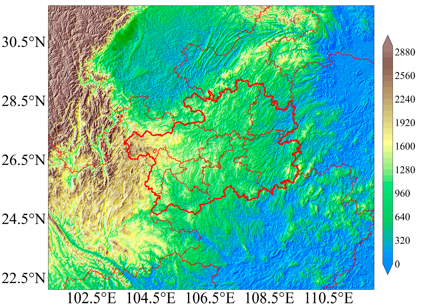
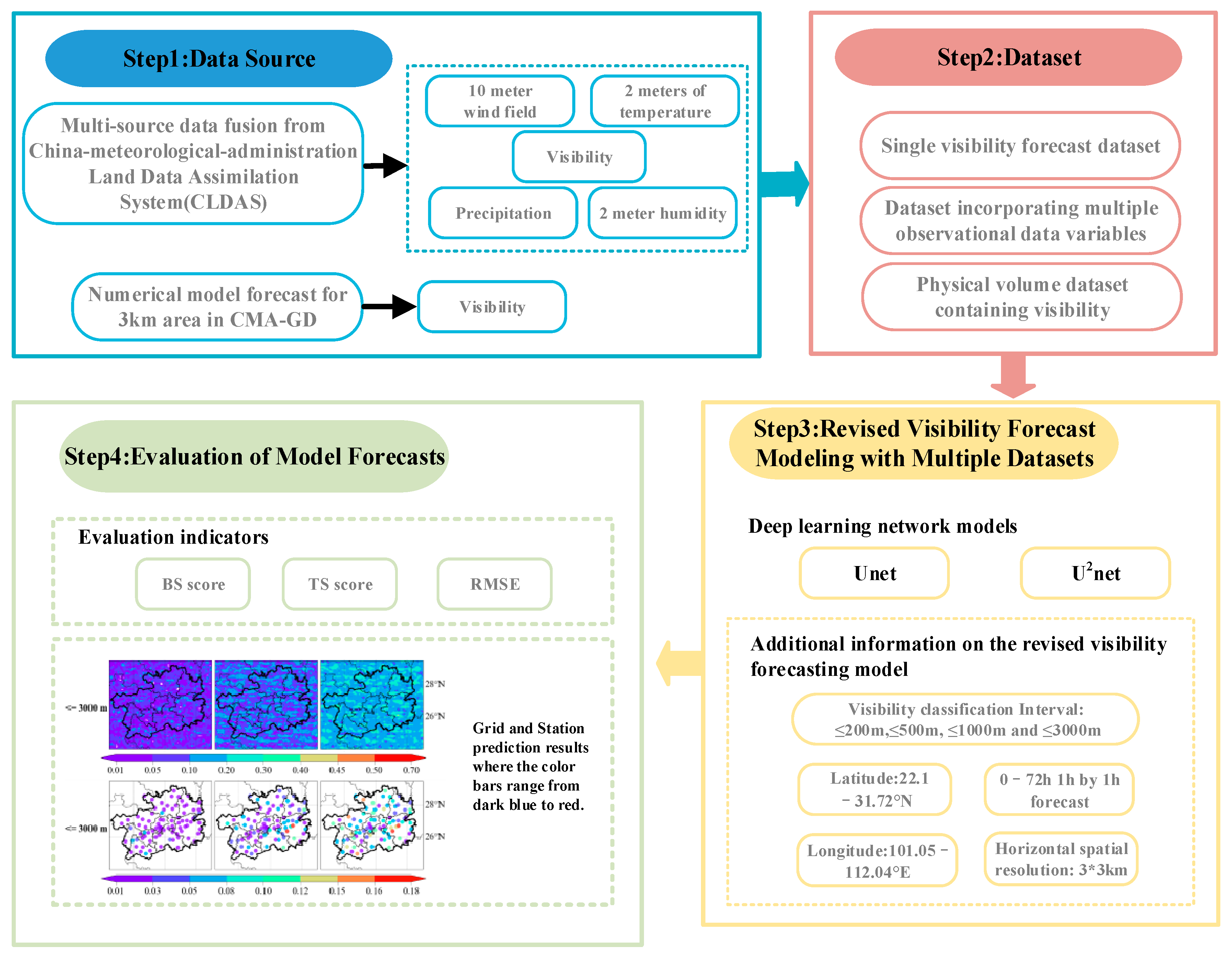
Guizhou lies on a slope from the Tibetan Plateau to the hilly areas of eastern China, and the karsts within its borders make it one of the most prone provinces to meteorological disasters, owing to the significant climatic variations and complex weather changes in different parts of the country. Guizhou is the only province in China with no plains and its topography varies greatly, with a distribution characterized by a “high in the west and low in the east” pattern (Figure 1). The conditions under which low visibility occurs in Guizhou vary, with frontal fog in the central–western and high-altitude regions and radiation fog in the eastern and northern parts of the province, which makes it challenging to forecast visibility in the province. Low-visibility weather is typical in Guizhou and has drawn considerable attention from the local public. Therefore, the region’s meteorological departments have placed particular emphasis on monitoring and forecasting low-visibility weather. However, Guizhou Province only has 84 national meteorological stations to monitor visibility, which is insufficient to comprehensively represent the visibility conditions across the province. In order to enable more detailed visibility forecasting for Guizhou, this study utilized the gridded observational data and the CMA-GD model output obtained from the China Meteorological Administration (CMA) Information Center to construct three visibility datasets to examine the impact of input data on the visibility forecasting capability. More specifically, to improve visibility forecasting in Guizhou, the Unet and U2net architectures were applied to establish visibility forecasting models for Guizhou Province based on multi-variable datasets. The threat score (TS), bias score (BS), and the root-mean-square error (RMSE) were used to evaluate the performance of visibility forecasting models.
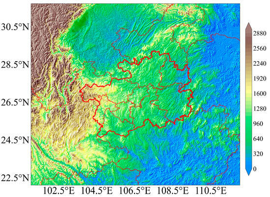
Figure 1.
Topographical map of the study area.
2. Data and Methodology
2.1. Data
This study employed hourly CMA Land Data Assimilation System (CLDAS) multi-source merged grid observation data, including visibility, precipitation, 10 m wind direction and speed, and 2 m humidity and temperature. The dataset had a horizontal resolution of 3 km. We obtained the CLDAS data from the CMA Information Center.
The CMA-GD model provided an hourly visibility forecast for the coming 72 h with a horizontal resolution of 3 km, the outputs of which we also obtained from the CMA Information Center.
The study region (22.1°–31.72° N, 101.05°–112.04° E) covered Guizhou Province, and the study period encompassed by the CLDAS observational data and CMA-GD model data spanned from 00:00 1 January 2022 to 23:00 30 June 2023.
2.2. Characteristics of the Visibility Data
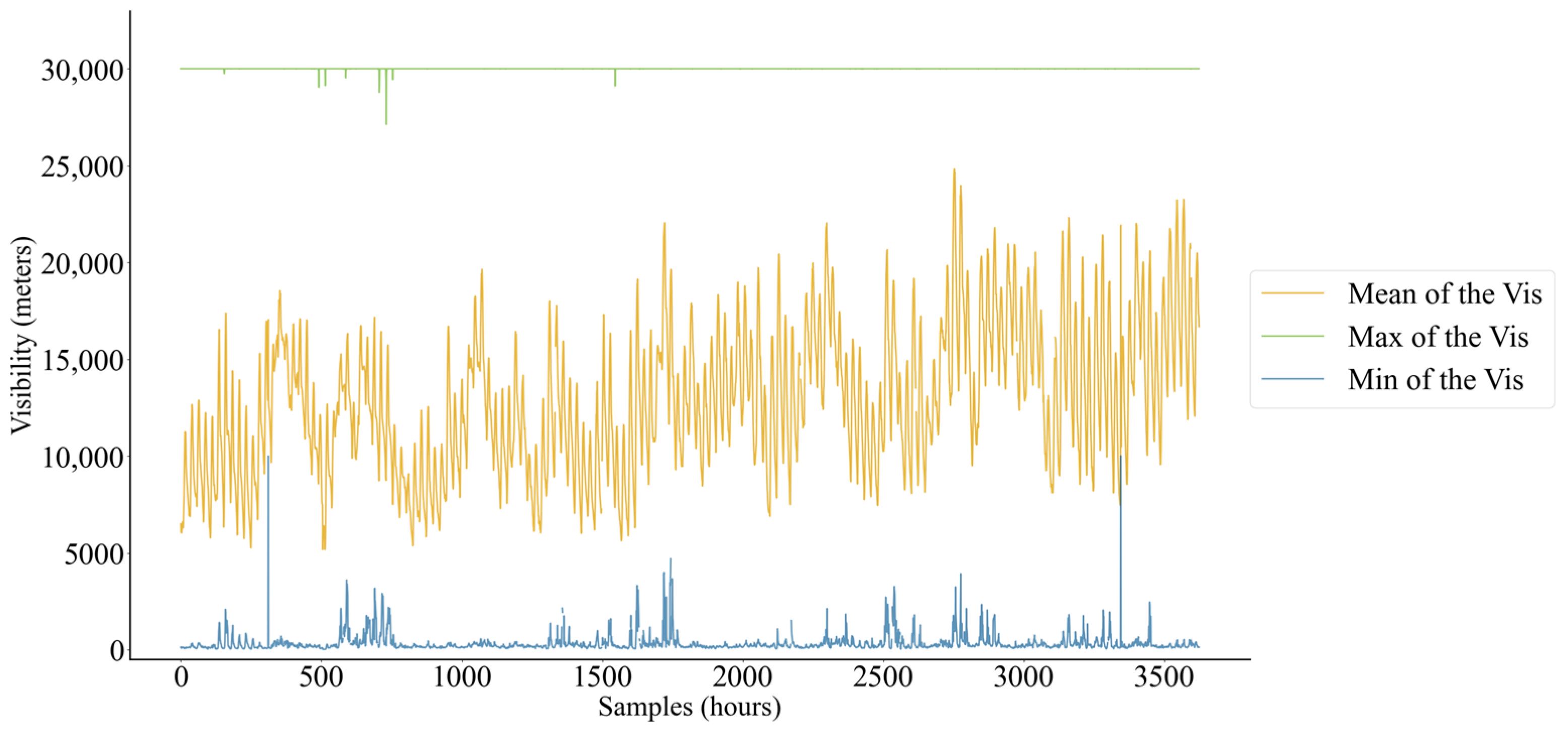
Figure 2 shows the characteristics of the visibility data for the validation set with a total sample size of 4344. Most of the samples in the study area had a maximum visibility of 30,000 m, and the mean values were mainly concentrated between 8000 and 15,000 m. Visibility minima were mainly concentrated below 500 m, with 1725 samples documenting visibility ≤200 m representing 39.71% of all samples and the number of samples with visibility ≤500 m being 3078 representing 70.86% of all samples, together indicating a relatively high quantity of low-visibility sample data (Figure 3). Therefore, the validation dataset used in this study was sufficient for evaluating the low-visibility forecasting ability of the model, meaning the evaluation results presented in this paper were both objective and effective.
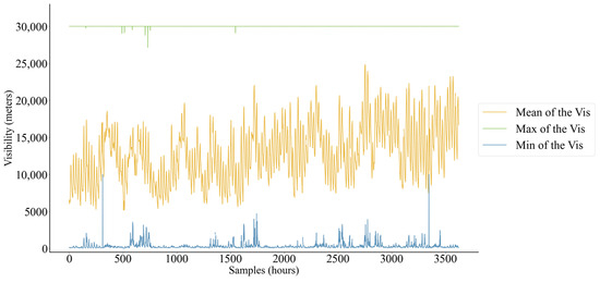
Figure 2.
Characteristics of the visibility data, with maximum visibility shown in green, minimum in blue, and the mean in yellow.
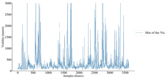
Figure 3.
Characteristics of visibility minima.
2.3. Methodology
2.3.1. Unet
For common forecasting tasks based on meteorological grid-point data, the conventional convolutional fully connected layer structure of the CNN networks could be replaced with the convolutional upsampling structure of a fully convolutional network (FCN). The FCN structure used an upsampling layer to enhance the global feature spatial information of the source data and a long jump connection to fuse the prediction layer and shallow features in an element-by-element summation to achieve an accurate prediction of the grid field data. This study established a visibility prediction model for Guizhou Province based on meteorological data using Unet and U2net as the basis (Figure 4). Unlike FCN, Unet could achieve greater detail to be captured and a small-sample learning capability by attenuating the number of feature channels while the decoder upsampled at a hierarchical level, and by upsampling at a hierarchical level through a long jump connection with the encoder corresponding to the feature data for matrix splicing and fusion [25,29].
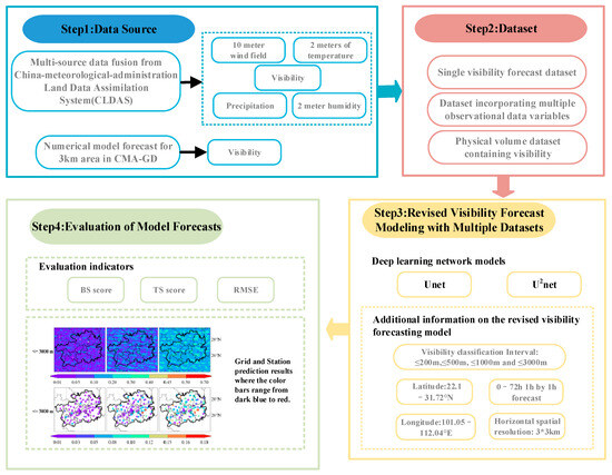
Figure 4.
Visibility forecasting model framework.
For the visibility prediction experiments carried out in this study, the network model data were processed as follows (taking Unet as an example, in which the Unet network had an encoder on the left and a decoder on the right): The encoder operation involved inputting a dataset consisting of multi-variable meteorological data (visibility, precipitation, 10 m wind direction and speed, 2 m humidity and temperature, and CMA_GD model data) into the model. The feature map size of the grid data was then changed to half its original size by modeling the 3 × 3 convolutional structure and ReLU activation function, as well as the maximum pooling operation. The decoder took the data processed using the encoder and doubled the size of the feature map by a 2 × 2 deconvolution. The cascade operation was implemented between the encoder and the decoder through a long jump connection, and the outputs of the convolutional layers were transferred to the decoder before the pooling operation of the encoder. Finally, the final visibility regression prediction was obtained with a 1 × 1 convolutional layer.
2.3.2. Evaluation Metrics
To evaluate the performance of each visibility forecasting model proposed in this study, we used the TS to evaluate the ability of the models to predict the occurrence of visibility events correctly. In this case, the TS measured the fractions of events that were correctly predicted. It ranged from 0 to 1, with 1 being a perfect score. The BS, meanwhile, was used to evaluate the overall accuracy of the probabilistic forecasts. The BS measured the mean squared difference between the forecast probability and the observed outcome. Moreover, the root-mean-square error (RMSE) was also used to assess model performance.
The TS, BS, and RMSE were calculated as follows:
where is the number of correctly forecast stations (events), is the number of false-alarm stations (events), represents the number of missed-forecast stations (events), is the number of samples, is the observed value, and is the forecast value. Evaluating the TS, BS, and RMSE of each model was performed for different visibility classifications: ≤200 m, ≤500 m, ≤1000 m, and ≤3000 m.
3. Datasets and Visibility Forecast Models
In order to increase the sample size, the missing data were estimated using neighboring points, which is a widely used approach in weather operations. The datasets were normalized by rescaling the data from 0 to 1 for the practical training of the deep learning models.
3.1. Unet-Based Visibility Forecasting Model Using Observational and Model Visibility Data
Based on the CLDAS and CMA-GD data, a visibility dataset (dataset I) was built using an input–output mapping method of “24 frames → 24 frames”, with data elements being visibility only. Then, a Unet-based visibility forecasting model (Unet_VToV) for Guizhou Province was trained and established, providing hourly forecasts at 0 to 72 h lead times with a horizontal resolution of 3 km.
3.2. Unet-Based Visibility Forecasting Model Using Multiple Observational Meteorological Variables
The CLDAS-merged multiple-meteorological-variable dataset (dataset II) included the following grid-based observational data variables: visibility, precipitation, 10 m wind direction and speed, and 2 m humidity and temperature. It is important to note that this dataset did not include any visibility forecast data from the CMA-GD model. We constructed a dataset using a “24 frames → 24 frames” input–output mapping approach. Then, the Unet architecture parameters were tuned and optimized to establish an hourly visibility forecasting model (Unet_NVToV) for Guizhou Province, covering a 0–72 h forecast range.
3.3. Unet- and U2net-Based Visibility Forecasting Model Using Multiple Observational Meteorological Variables and CMA-GD Visibility
Using the merged multiple meteorological variable dataset mentioned in Section 3.2 and the visibility forecast data from the CMA-GD model (dataset III), a Unet-based visibility forecasting model (Unet_PVToV) was established using the “24 frames → 24 frames” input–output mapping approach to provide hourly forecasts for Guizhou Province, covering a 0–72 h forecast range. Furthermore, a nested network architecture was introduced to construct a visibility forecasting model using the U2net architecture (U2net_PVToV).
4. Evaluation of Visibility Forecasting Models
The Unet-based visibility forecasting models were established using the three datasets (datasets I–III) mentioned in Section 3.1, Section 3.2 and Section 3.3, respectively. Each dataset was divided into training, validation, and testing with a 16:1:9 ratio. The training set covered the period from 1 January 2022 00:00 to 31 December 2022 23:00, resulting in 8784 samples. The testing set covered 1 January 2023 00:00 to 30 June 2023 23:00, generating 4344 samples for the model evaluation. The three datasets were input variables, and visibility was the output (Step1 and Step2 in Figure 4). The Unet and U2net architectures performed hourly visibility forecasts with 0–72 h lead times (Step3 in Figure 4). In addition, each hourly forecast of the visibility corresponded to a separate forecast model. The TS and BS were used to comprehensively evaluate and compare the performance of the different forecasting models, considering both grid-based and station-based assessments (Step4 in Figure 4). For the station-based evaluation of the models, we used the observed visibility values from the weather stations and the forecast values from the model grid closest to the station. The final scores for each model were calculated as the average of the 08:00 and 20:00 forecast performances. The visibility forecasting models were evaluated across multiple visibility classifications: ≤200 m, ≤500 m, ≤1000 m, and ≤3000 m. The verification was conducted for the 0–72 h forecasts with a 3 h interval.
4.1. Evaluation of the Unet-Based Visibility Forecasting Model
4.1.1. Grid-Based Assessments of Unet-Based Models
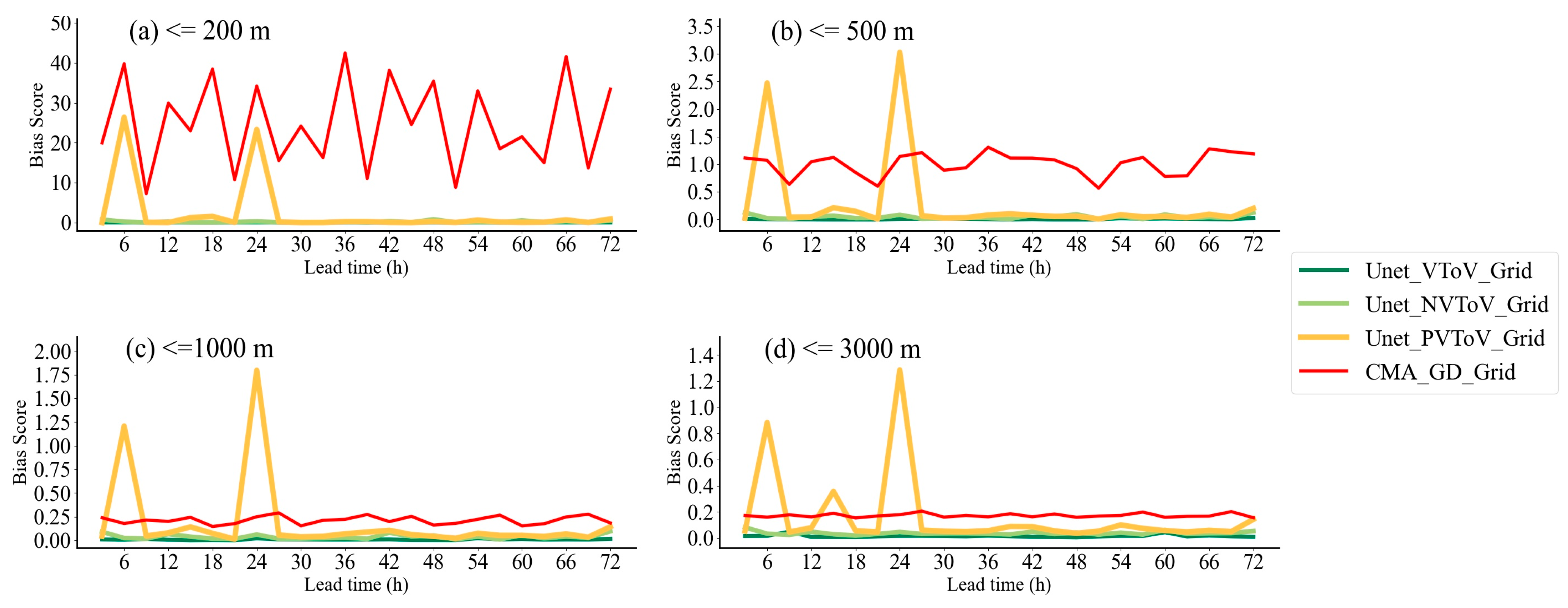
Figure 5 shows the gridded distributions of the TS of the Unet-based (Unet_VToV, Unet_NVToV, and Unet_PVToV) and CMA_GD visibility forecasting models. Unet_VToV had a higher TS (dark green lines in Figure 5) than CMA_GD (red lines) in the visibility classifications of ≤200 m and ≤500 m for the predictions at 24–30 h and 54–63 h lead times. Conversely, for the ≤1000 m and ≤3000 m visibility classifications, the TS of Unet_VToV was generally lower than CMA_GD, with a maximum decrease of 0.02. The results indicated that the forecasting performance of Unet_VToV was inferior to the original CMA_GD model.
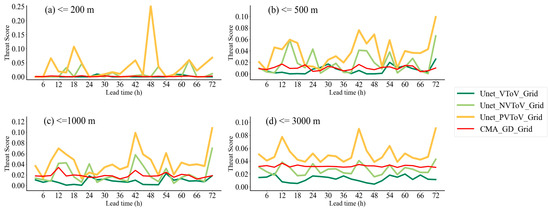
Figure 5.
Threat scores of the visibility forecasting from three Unet-based and CMA-GD models. Results for the Unet_VToV model are shown in dark green, Unet_NVToV in light green, Unet_PVToV in yellow, and CMA_GD in red.
Unet_NVToV (light green lines) had a higher TS in the ≤200 m, ≤500 m, and ≤1000 m visibility classifications, outperforming Unet_VToV and surpassing CMA_GD in most of the predictions. In the ≤3000 m visibility classification, the TS of Unet_NVToV was higher than that of Unet_VToV, but 0.02 lower than that of CMA_GD.
For the Unet_PVToV model (yellow lines), there was a significant improvement in the TS for all visibility classifications. The TSs for nearly all forecast ranges were higher than those of Unet_VToV, Unet_NVToV, and CMA_GD, with the maximum TS reaching 0.25 for the ≤200 m visibility classification (Figure 5a). Note that the TS improvements in Unet_PVToV were less stable for the ≤200 m visibility classification, with only a few forecasts showing substantial improvements, indicating a relatively lower model stability in heavy-fog forecasting.
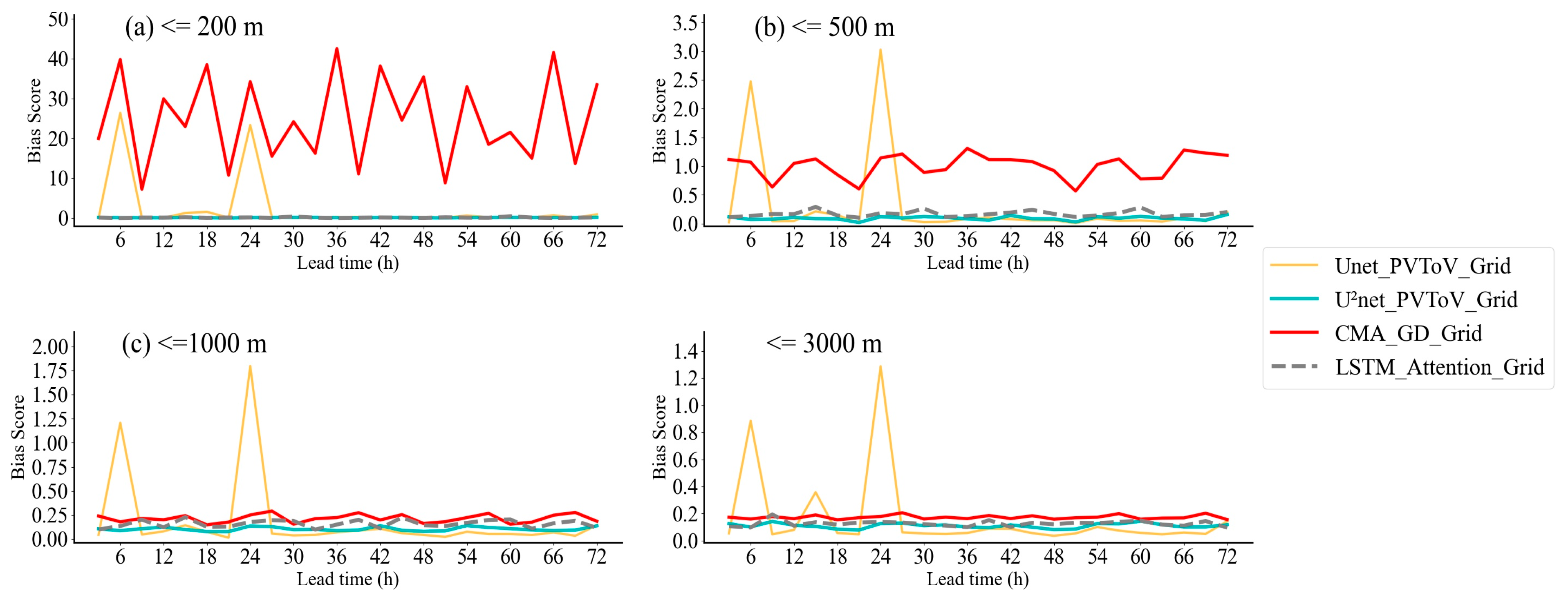
Figure 6 shows the BSs of the visibility forecasting models. Unet_VToV and Unet_NVToV had much lower BSs than CMA_GD for all visibility classifications, with the best performance seen for visibility below 200 m. Again, Unet_PVToV had a lower BS than CMA_GD did, which indicated that Unet_PVToV had smaller forecast errors. Especially in the ≤200 m visibility classification, the average BS was reduced by 20. However, Unet_PVToV had some high BSs for predictions with a lead time of less than 27 h, which suggested some significant errors during this period. In general, the improvement in the BS of Unet_PVToV was not as substantial as the improvements found in the TS evaluation. While Unet_PVToV showed a significant improvement in forecast accuracy, as shown by the TS, the larger BS suggested that Unet_PVToV still struggled with specific forecast periods, with some more significant errors during these periods.

Figure 6.
Similar to Figure 5, but for the bias score evaluations.
4.1.2. Station-Based Assessments of Unet-Based Models
Figure 7 shows the TSs of the visibility forecasting models at all the weather stations in Guizhou Province. Unet_VToV had higher TSs than CMA_GD in most of the predictions for the visibility classifications of ≤200 m, ≤500 m, and ≤1000 m. However, it had lower TSs than CMA_GD in the 27–33 h and 66–72 h forecasts. For the ≤3000 m visibility classification, the TSs of Unet_VToV were not uniformly larger than those of CMA_GD, with notable decreases compared to CMA_GD in the 6–15-h, 27–36-h, and 51–60 h forecasts. Unet_NVToV had larger TSs than Unet_VToV, with a maximum increase of 0.03, outperforming CMA_GD. However, within the first 15 h of the ≤3000 m visibility condition, Unet_NVToV had a lower TS than Unet_VToV and CMA_GD. Unet_PVToV had higher station-based TSs than Unet_NVToV (maximum increase of 0.06) and outperformed Unet_VToV_Sta. Unet_PVToV effectively enhanced the model performance and increased the TSs of forecasts with a lead time of less than 15 h.
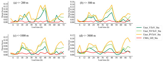
Figure 7.
Threat score evaluations of visibility forecasting from three Unet-based models and the CMA-GD model at weather stations. Results for Unet_VToV are shown in dark green, Unet_NVToV in light green, Unet_PVToV in yellow, and CMA_GD in red.
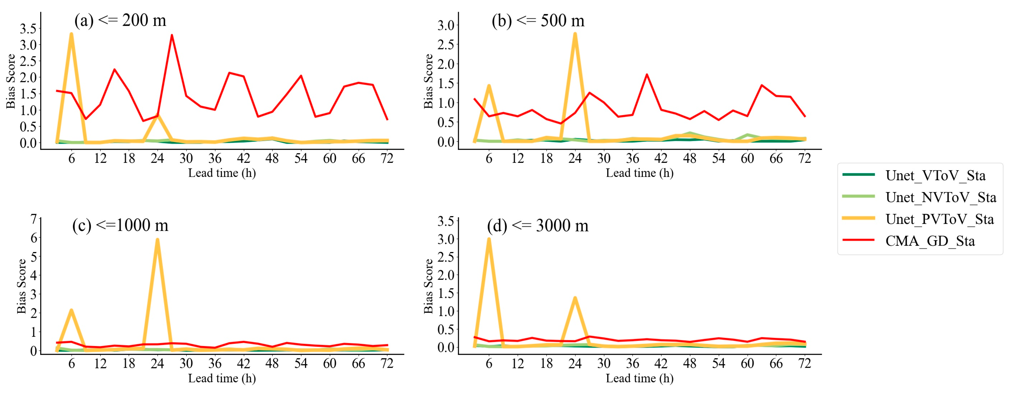
Figure 8 shows the BSs of the visibility forecasting models. The BS evaluations of Unet_VToV and Unet_NVToV at weather stations were similar to those of the grid-based evaluation. The BSs of Unet_VToV and Unet_NVToV were significantly lower than those of CMA_GD for all visibility classifications, with a maximum reduction of approximately 3.5. The BS of Unet_PVToV at stations was similar to that of Unet_PVToV over the model grid, which had a notable reduction compared to CMA_GD. However, the improvement for Unet_PVToV was less substantial than that found in Unet_VToV and Unet_NVToV. Moreover, Unet_PVToV had a high BS for all visibility classifications for the forecasts with a lead time of less than 27 h, which indicated significant forecast errors during this period.
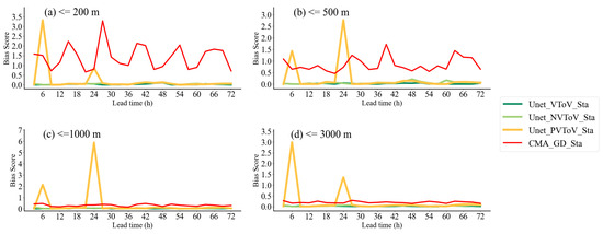
Figure 8.
Similar to Figure 7, but for the bias score evaluations.
The evaluations on model grids and at weather stations showed that the TS of visibility forecasts increased by adopting the Unet-based model and including more meteorological variables. Unet_PVToV achieved considerably higher TSs than the other models for the ≤500 m, ≤1000 m, and ≤3000 m visibility classifications, which demonstrated good forecasting capabilities. However, the TS improvement for Unet_PVToV was less pronounced for the ≤200 m visibility classification, where the model was less robust. Moreover, the BS evaluation indicated significant forecast errors within the 72 h forecast range. Overall, the model incorporating the multi-variable physical quantities, including visibility, performed better.
4.2. Evaluation of the U2net-Based Visibility Forecasting Model
To further enhance the TS and decrease the BS of the Unet-based forecasting models, a model based on the U2net architecture using the multi-variable physical quantity dataset with CMA_GD visibility (dataset III) was constructed and evaluated.
4.2.1. Grid-Based Assessments
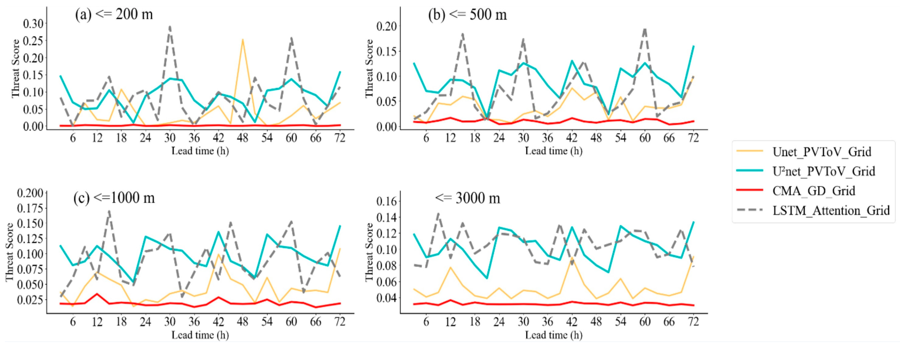
Figure 9 shows the TSs of the Unet- and U2net-based visibility forecasting models and the CMA_GD model. By introducing the nested U2net model architecture, the U2net_PVToV model showed a 0.06 higher TS than Unet_PVToV in the ≤500 m, ≤1000 m, and ≤3000 m visibility classifications. U2net_PVToV had a much higher TS than CMA_GD at various lead times. Furthermore, for the ≤200 m visibility classification, U2net_PVToV_Grid had higher TSs than CMA_G and Unet_PVToV. U2net_PVToV was more robust, with a substantial improvement in the TS. Compared to LSTM_Attention_Grid, the TS of LSTM_Attention_Grid was better than that of U2net_PVTo_V_Grid at individual times, but, overall, the TS of U2net_PVTo_V_Grid performed a little better, with better model stability.
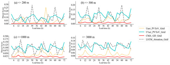
Figure 9.
Threat scores of the visibility forecasting models based on the Unet (yellow lines) and U2net (cyan lines) architectures, along with the CMA_GD model (red lines) and LSTM_Attention model (grey lines).
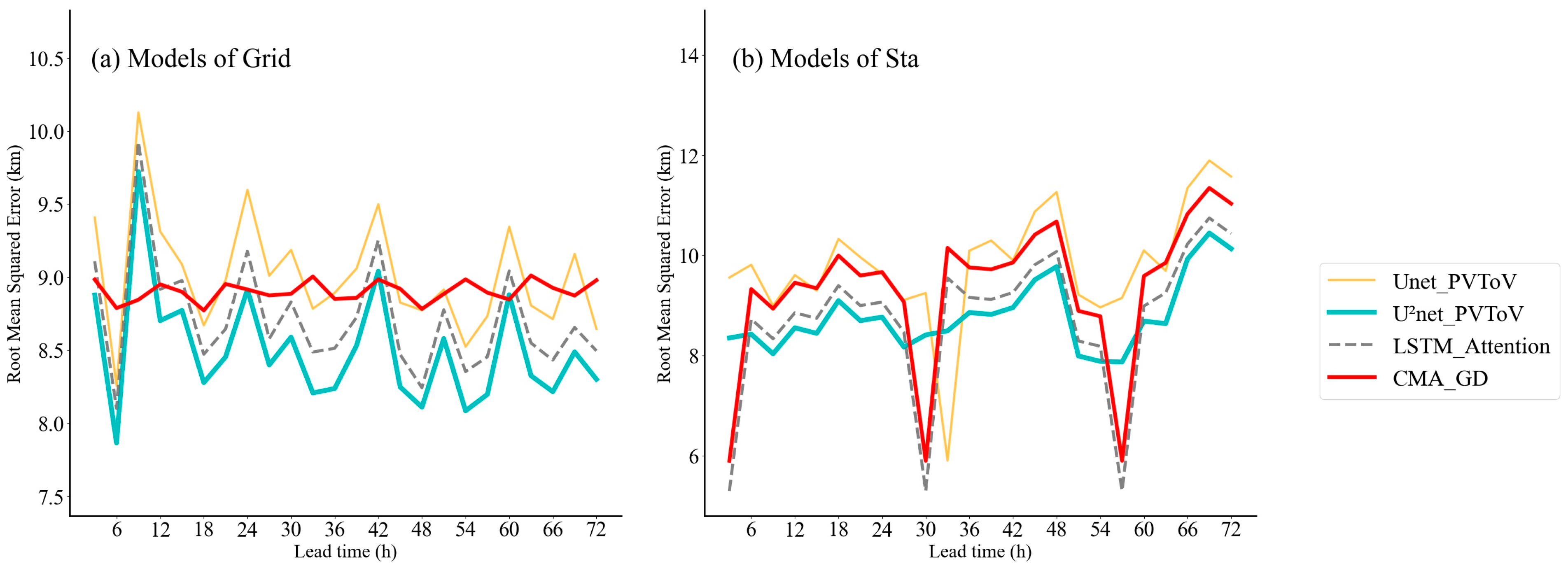
As for the BS of the visibility forecast models, shown in Figure 10, we could see that U2net_PVToV significantly decreased the forecast errors within the 72 h prediction found in Unet_PVToV. U2net_PVToV had an overall low BS (<0.2) for all visibility classifications, which constituted a notable reduction in the BS compared to Unet_PVToV and CMA_GD, with an average decrease of 0.3 to 1.0. The BS of LSTM_Attention_Grid was close to that of U2net_PVToV, but the BS of U2net_PVToV performed better in the ≤500 m and ≤1000 m visibility classifications. The RMSE results showed a significant improvement for U2net_PVToV over Unet_PVToV and CMA_GD, and an overall reduction in RMSE over LSTM_Attention (Figure 11). These results demonstrated that the U2net-based model could increase the TS of visibility forecasts and reduce forecast errors, thereby strengthening the overall stability of the model.
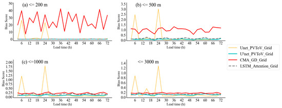
Figure 10.
Bias scores of the visibility forecasting models based on the Unet (yellow lines) and U2net (cyan lines) architectures, along with the CMA_GD model (red lines) and LSTM_Attention model (grey lines).
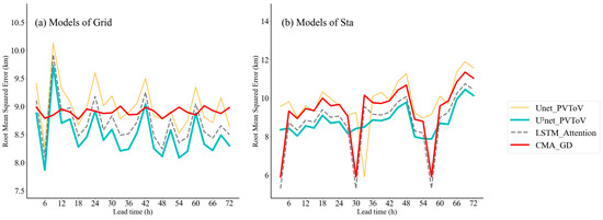
Figure 11.
RMSE of the visibility forecasting models based on the Unet (yellow lines) and U2net (cyan lines) architectures, along with the CMA_GD model (red lines) and LSTM_Attention model (grey lines).
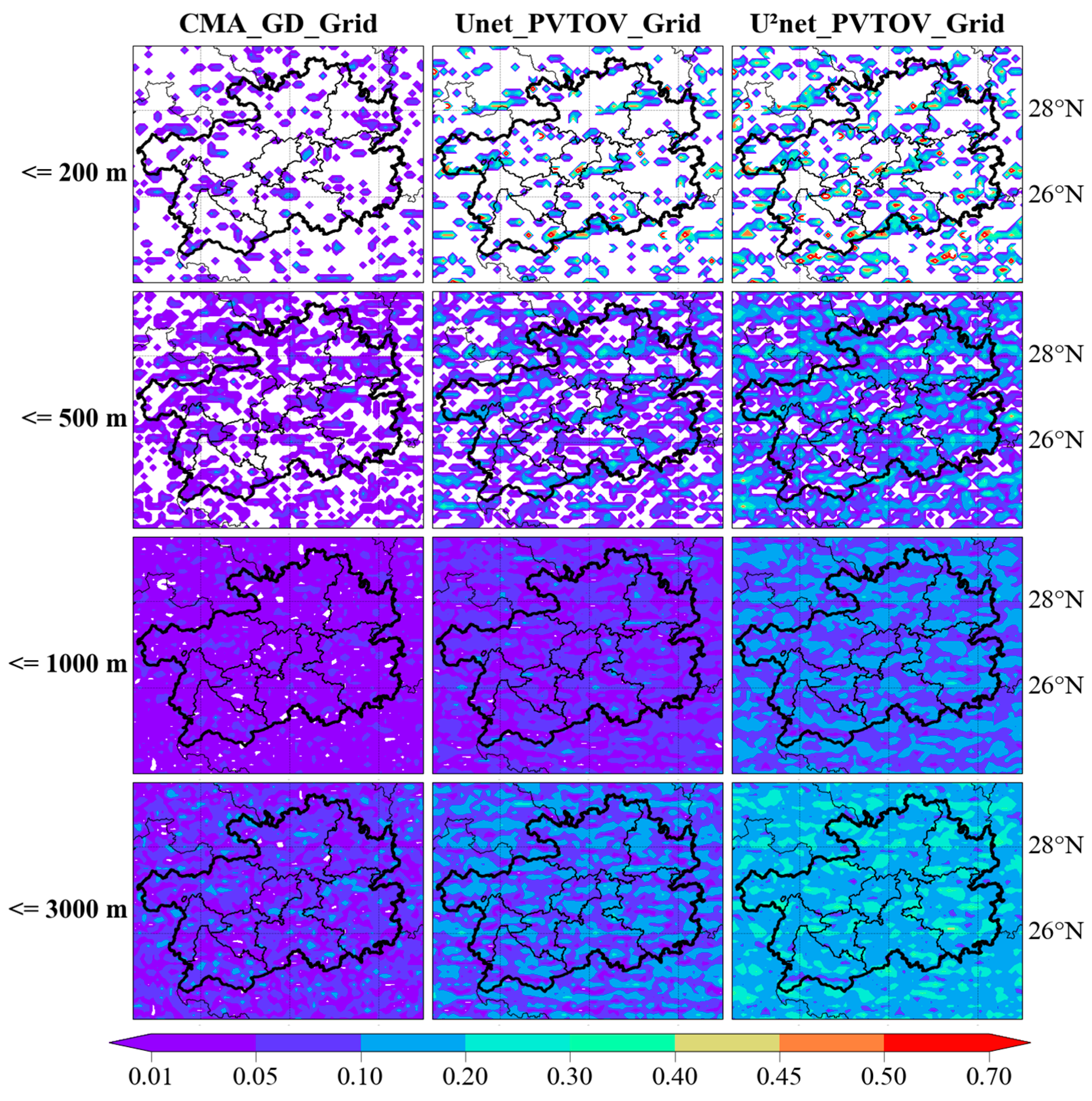
To further illustrate the forecasting skill improvements by introducing the U2net architecture, the spatial distributions of the TS for the models in Guizhou Province are presented in Figure 12. As can be seen, CMA_GD had a TS ranging from 0.01 to 0.2, with the majority of the area having scores below 0.1, which indicated a poor forecasting performance of this model. Compared to CMA_GD, Unet_PVToV showed notable improvements in the ≤200 m visibility classification, with the TS reaching the range of 0.1 to 0.7. For the ≤500 m and ≤3000 m visibility classifications, Unet_PVToV produced an increase in the TS over some areas of Guizhou, reaching 0.1 to 0.2. There was no significant difference in the TS between CMA_GD and Unet_PVToV for the ≤1000 m visibility classification. In contrast, U2net_PVToV demonstrated substantial TS improvements for all visibility classifications. For the ≤200 m visibility classification, U2net_PVToV had a TS approximately three times higher than that of CMA_GD. The TS of U2net_PVToV increased by a factor of three over CMA_GD, and its spatial coverage with a TS reaching 0.5 was wider than that of Unet_PVToV_Grid. For the other visibility classifications, U2net_PVToV also had higher TSs than CMA_GD and Unet_PVToV, especially for the ≤1000 m visibility classification, where the forecast performed better than that of Unet_PVToV.
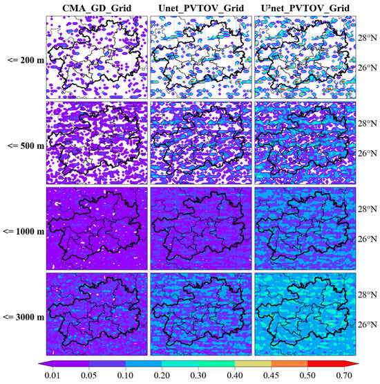
Figure 12.
Spatial distribution of the threat score of the forecast from (left) CMA_GD_Grid, (middle) Unet_PVTOV_Grid, and (right) U2net_PVTOV_Grid in Guizhou Province for different visibility classifications: (from top to bottom) ≤200 m, ≤500 m, ≤1000 m, and ≤3000 m.
In summary, introducing the nested U2net architecture substantially improved the TS of the visibility forecasting model. The TS of U2net_PVToV was able to reach 0.5–0.7 for the ≤200 m visibility classification, which indicated that the U2net-based model could better forecast low-visibility weather conditions. U2net_PVToV also reduced the significant forecast errors within the 72 h prediction found in the Unet-based model. Moreover, the U2net-based model significantly reduced the BS, diminishing the overall forecast errors and improving the model’s stability. U2net_PVToV could provide more reliable visibility forecast products in Guizhou Province, especially in areas lacking ground-based visibility observations.
4.2.2. Station-Based Assessments
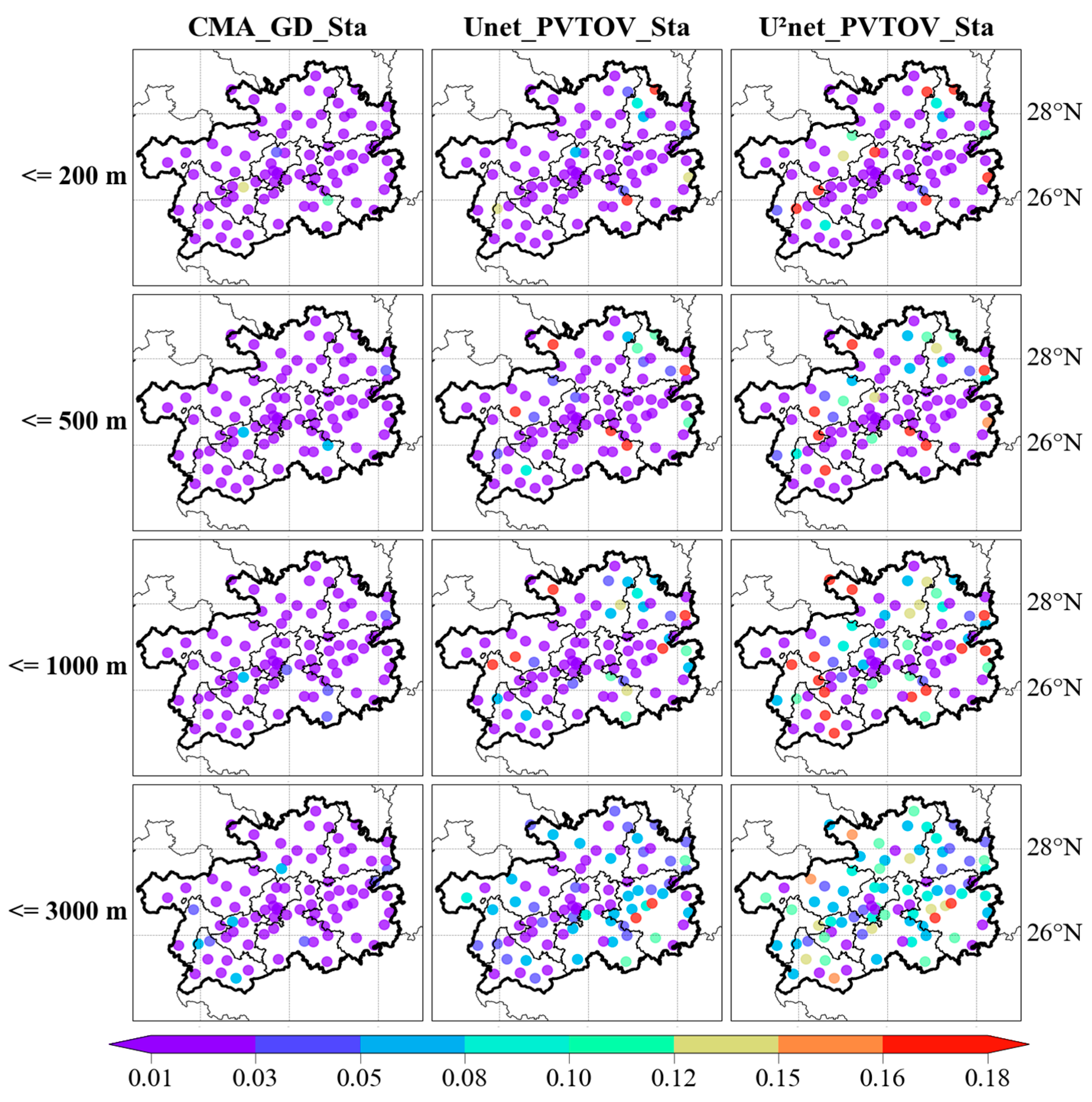
The evaluations of the models at stations were similar to those over model grids. The station-averaged TS (BS, RMSE) was higher (lower) at various prediction times in U2net_PVToV than Unet_PVToV and CMA_GD. To assess the model performance over different areas, the TS values for the different models at each weather station are presented in Figure 13. CMA_GD had a low TS, ranging from 0.01 to 0.05, across Guizhou Province, with most stations experiencing a TS below 0.03. This indicated a generally poor forecast performance of CMA_GD. For Unet_PVToV, the TS was higher in the eastern, southern, and northwestern parts of Guizhou for the ≤500 m, ≤1000 m, and ≤3000 m visibility classifications than for CMA_GD. However, in the ≤200 m visibility range, improvements were less pronounced. U2net_PVToV had a significantly higher TS for all visibility classifications. Especially in the ≤3000 m visibility classification, the TS tripled compared to CMA_GD at most stations. The areas with a higher TS were in Guizhou’s southern, northern, and northwestern parts. It is worth noting that the improvements in TS for the low-visibility (≤200 m) classifications at stations were not as extensive as the evaluations over model grids (Figure 12).
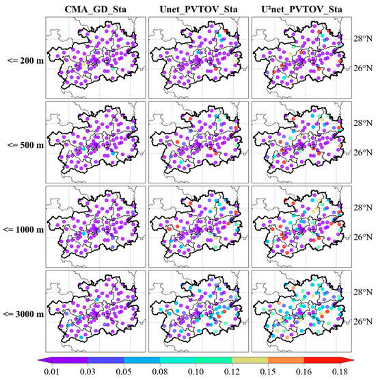
Figure 13.
Spatial distribution of the threat score for the (left) CMA_GD_Sta, (middle) Unet_PVTOV_Sta, and (right) U2net_PVTOV_Sta models at weather stations in Guizhou Province for different visibility classifications: (from top to bottom) ≤200 m, ≤500 m, ≤1000 m, and ≤3000 m.
The visibility forecasting model based on the U2net network architecture had significantly higher TSs and lower forecast errors. Moreover, the U2net-based model outperformed the Unet-based and CMA_GD models at various lead times and over different areas of Guizhou. While the U2net-based model delivered substantial improvements in the station-based visibility forecast evaluations, there was still room for further enhancements, particularly under low-visibility conditions at the stations.
4.3. Overall Evaluation of TS and BS
An overall evaluation of the models’ TSs taken over model grids and at weather stations is summarized in Table 1 and in Table 2 for the BSs. These comprehensive TS and BS evaluations highlighted the stepwise advancements in the forecasting capabilities achieved through the progressive refinements in the dataset compositions and the model architectures. Unet_PVToV significantly improved the skill scores compared to CMA_GD, with an average tripling of the TS for different visibility classifications. By introducing the nested U2net architecture and increasing the model depth, U2net_PVToV further increased the TS, with a doubling over Unet_PVToV, and all classification intervals had higher TSs than LSTM_Attention. Moreover, the model evaluations over model grids were better than those at weather stations.

Table 1.
Overall evaluation of the TS of the visibility forecasting models over model grids and at weather stations in Guizhou Province.
Table 2.
Overall evaluation of the BS of the visibility forecasting models over model grids and at weather stations in Guizhou Province.
Unet_PVToV had higher TSs than Unet_VTOV and Unet_NVTOV. The higher BS of Unet_PVToV indicated that the model became less stable when the CMA_GD output was included. U2net_PVToV increased the TS and decreased the BS, which resulted in more robust and consistent visibility forecasting capabilities.
5. Conclusions
This study established visibility forecast models for Guizhou Province by utilizing the Unet and U2net architectures based on three datasets. Model performances were evaluated using the temporal evolution and spatial distribution of the TSs and BSs of forecasts with lead times of 0–72 h over model grids and at weather stations. The key findings were as follows:
The Unet-based visibility forecasting model using the multi-variable physical quantity dataset could significantly increase the TS compared to the CMA-GD model, with a more than threefold increase. This approach also enhanced the forecast stability. However, the Unet-based models had larger BSs than the CMA-GD model.
The nested U2net architecture, which deepened the neural network structure, could strengthen the model’s ability to extract physical field features and increase the TS, achieving a more than sixfold increase over the CMA-GD model. In addition, by introducing the U2net architecture, the model further improved the TS by approximately a factor of two compared to the Unet model, and significantly reduced the BS. In particular, in terms of the TS, the U2net-based model performed the best at the ≤200 m visibility threshold, with a more than eightfold increase over the CMA-GD model. The spatial distribution of the TS showed that the U2net-based model performed better at the model grid scale than at individual weather stations. Compared to the Unet-based and LSTM_Attention model, the U2net-based model lowered the overall BS and RMSE, reducing significant prediction errors. The U2net-based model could improve the accuracy and stability of the visibility forecast model. It was the best model we ever built for predicting visibility.
6. Discussion
The visibility forecasting model developed in this study using the multi-variable physical quantity dataset and the U2net architecture provides a significant reference value for operational applications. However, the low-visibility (≤200 m) forecast at stations still requires improvements. Besides the meteorological variables, the performance of the visibility forecast can be affected by the terrain [32]. Future research should aim to integrate high-resolution terrain information into training data appropriately. Expanding the sample size and optimizing the U2net architecture are needed to enhance the model performance and decrease the forecasting error.
Author Contributions
Methodology, D.H. and Y.T.; investigation, Y.W. and D.H.; validation, Y.T. and Y.W.; software, D.K. and D.H.; writing—original draft preparation, D.H., W.Z. and J.Y.; writing—review and editing, J.Y., D.K. and H.L.; supervision, D.H., D.K. and F.W. All authors have read and agreed to the published version of the manuscript.
Funding
The study was jointly supported by the China Meteorological Administration Review and Summarize Special Project (grant no.: FPZJ2024-116), Guizhou Meteorological Bureau Provincial-Municipal Joint Fund Project (grant no.: Qianqi Kehe SS [2023]38), Qiannan Prefecture Science and Technology Bureau Science and Technology Plan Project (grant no.: 2023-4-88), Guizhou Provincial Department of Science and Technology Science and Technology Plan Project (grant no.: Qiankehe Basic-ZK [2023]457), Qiannan Prefecture Meteorological Bureau Research Project (grant no.: 2019-15), and Gansu Youth Science and Technology Fund Program (grant no.: 22JR5RA752), Research on rain nest monitoring and forecasting technology in Guizhou (grant no.: Qianqi Kehe TD [2024]01).
Institutional Review Board Statement
Not applicable.
Informed Consent Statement
Not applicable.
Data Availability Statement
The observation data used in this study were provided by the Guizhou Meteorological Information Center and are not public in nature. The dataset was newly established in this study.
Conflicts of Interest
The authors declare no conflicts of interest.
References
- Doyle, M.; Dorling, S. Visibility trends in the UK 1950–1997. Atmos. Environ. 2002, 36, 3161–3172. [Google Scholar] [CrossRef]
- Belo-Pereira, M.; Santos, J. A persistent wintertime fog episode at Lisbon airport (Portugal): Performance of ECMWF and AROME models. Meteorol. Appl. 2016, 23, 353–370. [Google Scholar] [CrossRef]
- Codur, M.Y.; Kaplan, N.H. Increasing the visibility of traffic signs in foggy weather. Fresenius Environ. Bull. 2019, 28, 705–709. [Google Scholar]
- Erkan, A.; Hoffmann, D.; Kreß, N.; Vitkov, T.; Kunst, K.; Peier, M.A.; Khanh, T.Q. Required Visibility Level for Reliable Object Detection during Nighttime Road Traffic in Non-Urban Areas. Appl. Sci. 2023, 13, 2964. [Google Scholar] [CrossRef]
- Yang, Y.; Ge, B.; Chen, X.; Yang, W.; Wang, Z.; Chen, H.; Xu, D.; Wang, J.; Tan, Q. Wang. Impact of water vapor content on visibility: Fog-haze conversion and its implications to pollution control. Atmos. Res. 2021, 256, 105565. [Google Scholar] [CrossRef]
- Cao, Y.; Xu, H.; Wu, H.; Lu, X.; Shen, S. The Commuting Patterns and Health Effects among Urban Residents in Low-Visibility Air Pollution Environments: An Empirical Study of Gaoyou City, China. Atmosphere 2023, 14, 1140. [Google Scholar] [CrossRef]
- Yang, C.-H.; Chen, P.-H.; Wu, C.-H.; Yang, C.-S.; Chuang, L.-Y. Deep learning-based air pollution analysis on carbon monoxide in Taiwan. Ecol. Inform. 2024, 80, 102477. [Google Scholar] [CrossRef]
- Deng, Z.; Wang, T.; Zheng, Y.; Zhang, W.; Yun, Y.-H. Deep learning in food authenticity: Recent advances and future trends. Trends Food Sci. Technol. 2024, 144, 104344. [Google Scholar] [CrossRef]
- Aizenstein, H.; Moore, R.C.; Vahia, I.; Ciarleglio, A. Deep Learning and Geriatric Mental Health. Am. J. Geriatr. Psychiatry 2024, 32, 270–279. [Google Scholar] [CrossRef]
- Li, Z.; He, Q.; Li, J. A survey of deep learning-driven architecture for predictive maintenance. Eng. Appl. Artif. Intell. 2024, 133, 108285. [Google Scholar] [CrossRef]
- Tang, C.; Wang, L.; Wei, Y.; Wu, P.; Wei, H. Time-Frequency Domain Variation Analysis and LSTM Forecasting of Regional Visibility in the China Region Based on GSOD Station Data. Atmosphere 2023, 14, 1072. [Google Scholar] [CrossRef]
- Duddu, V.R.; Pulugurtha, S.S.; Mane, A.S.; Godfrey, C. Back-propagation neural network model to predict visibility at a road link-level. Transp. Res. Interdiscip. Perspect. 2020, 8, 100250. [Google Scholar] [CrossRef]
- Chaabani, H.; Kamoun, F.; Bargaoui, H.; Outay, F.; Yasar, A.-U.-H. A Neural network approach to visibility range estimation under foggy weather conditions. Procedia Comput. Sci. 2017, 113, 466–471. [Google Scholar] [CrossRef]
- Liu, Z.; Chen, Y.; Gu, X.; Yeoh, J.K.; Zhang, Q. Visibility classification and influencing-factors analysis of airport: A deep learning approach. Atmos. Environ. 2022, 278, 119085. [Google Scholar] [CrossRef]
- Ortega, L.C.; Otero, L.D.; Solomon, M.; Otero, C.E.; Fabregas, A. Deep learning models for visibility forecasting using climatological data. Int. J. Forecast. 2023, 39, 992–1004. [Google Scholar] [CrossRef]
- Chen, Y.; Li, X.; Zhao, S. A Novel Photovoltaic Power Prediction Method Based on a Long Short-Term Memory Network Optimized by an Improved Sparrow Search Algorithm. Electronics 2024, 13, 993. [Google Scholar] [CrossRef]
- Zhang, F.; Lai, C.; Chen, W. Weather Radar Echo Extrapolation Method Based on Deep Learning. Atmosphere 2022, 13, 815. [Google Scholar] [CrossRef]
- Ji, L.; Fu, C.; Ju, Z.; Shi, Y.; Wu, S.; Tao, L. Short-Term Canyon Wind Speed Prediction Based on CNN—GRU Transfer Learning. Atmosphere 2022, 13, 813. [Google Scholar] [CrossRef]
- Gao, L.; Yang, Y.-M.; Li, Q.; Ham, Y.-G.; Kim, J.-H. Deep Learning for Predicting Winter Temperature in North China. Atmosphere 2022, 13, 702. [Google Scholar] [CrossRef]
- Peláez-Rodríguez, C.; Pérez-Aracil, J.; de Lopez-Diz, A.; Casanova-Mateo, C.; Fister, D.; Jiménez-Fernández, S.; Salcedo-Sanz, S. Deep learning ensembles for accurate fog-related low-visibility events forecasting. Neurocomputing 2023, 549, 126435. [Google Scholar] [CrossRef]
- Peláez-Rodríguez, C.; Pérez-Aracil, J.; Casanova-Mateo, C.; Salcedo-Sanz, S. Efficient prediction of fog-related low-visibility events with Machine Learning and evolutionary algorithms. Atmos. Res. 2023, 295, 106991. [Google Scholar] [CrossRef]
- Zhang, X.; Du, H.; Song, G.; Bao, F.; Zhang, Y.; Wu, W.; Liu, P. X-ray coronary centerline extraction based on C-Unet and a multifactor reconnection algorithm. Comput. Methods Programs Biomed. 2022, 226, 107114. [Google Scholar] [CrossRef]
- Zhang, Z.; Gao, L.; Li, P.; Jin, G.; Wang, J. DAUF: A disease-related attentional Unet framework for progressive and stable mild cognitive impairment identification. Comput. Biol. Med. 2023, 165, 107401. [Google Scholar] [CrossRef]
- Prasad, J.R.; Prasad, R.S.; Dhumane, A.; Ranjan, N.; Tamboli, M. Gradient bald vulture optimization enabled multi-objective Unet++ with DCNN for prostate cancer segmentation and detection. Biomed. Signal Process. Control. 2024, 87, 105474. [Google Scholar] [CrossRef]
- Yang, W.; Zhao, Y.; Li, Q.; Zhu, F.; Su, Y. Multi visual feature fusion based fog visibility estimation for expressway surveillance using deep learning network. Expert Syst. Appl. 2023, 234, 121151. [Google Scholar] [CrossRef]
- Qu, J.; Gao, Y.; Lu, Y.; Xu, W.; Liu, R.W. Deep learning-driven surveillance quality enhancement for maritime management promotion under low-visibility weathers. Ocean. Coast. Manag. 2023, 235, 106478. [Google Scholar] [CrossRef]
- Fernández, J.G.; Abdellaoui, I.A.; Mehrkanoon, S. Deep coastal sea elements forecasting using Unet-based models. Knowledge-Based Syst. 2022, 252, 109445. [Google Scholar] [CrossRef]
- Li, J.; Li, L.; Zhang, T.; Xing, H.; Shi, Y.; Li, Z.; Wang, C.; Liu, J. Flood forecasting based on radar precipitation nowcasting using U-net and its improved models. J. Hydrol. 2024, 632, 130871. [Google Scholar] [CrossRef]
- Qin, X.; Zhang, Z.; Huang, C.; Dehghan, M.; Zaiane, O.R.; Jagersand, M. U2-Net: Going deeper with nested U-structure for salient object detection. Pattern Recognit. 2020, 106, 107404. [Google Scholar] [CrossRef]
- Cheng, H.; Li, Y.; Li, H.; Hu, Q. Embankment crack detection in UAV images based on efficient channel attention U2Net. Structures 2023, 50, 430–443. [Google Scholar] [CrossRef]
- Liu, T.; Lu, Y.; Zhang, Y.; Hu, J.; Gao, C. A bone segmentation method based on Multi-scale features fuse U2Net and improved dice loss in CT image process. Biomed. Signal Process. Control. 2022, 77, 103813. [Google Scholar] [CrossRef]
- Liang, C.-W.; Chang, C.-C.; Hsiao, C.-Y.; Liang, C.-J. Prediction and analysis of atmospheric visibility in five terrain types with artificial intelligence. Heliyon 2023, 9, e19281. [Google Scholar] [CrossRef] [PubMed]


Disclaimer/Publisher’s Note: The statements, opinions and data contained in all publications are solely those of the individual author(s) and contributor(s) and not of MDPI and/or the editor(s). MDPI and/or the editor(s) disclaim responsibility for any injury to people or property resulting from any ideas, methods, instructions or products referred to in the content. |
© 2024 by the authors. Licensee MDPI, Basel, Switzerland. This article is an open access article distributed under the terms and conditions of the Creative Commons Attribution (CC BY) license (https://creativecommons.org/licenses/by/4.0/).