High-Resolution Modeling of Air Quality in Abidjan (Côte d’Ivoire) Using a New Urban-Scale Inventory

Abstract

In West African cities, the impacts of the air quality on the health of the population is expected to increase significantly in the near future. For the first time to our knowledge, we conducted a high-resolution modeling study over Abidjan (Côte d’Ivoire) using the WRF-Chem model and the simplified GOCART model to simulate carbonaceous aerosols BC and OC, sulfate, dust, sea salt, PM_2.5, and PM₁₀. The simulations were carried out during January and February 2019, a period over which there are databases of observations available. The DACCIWA inventory provided anthropogenic emissions at the regional scale, whereas a new emission inventory has been developed for the city of Abidjan. In 2019, the emissions were 4986.8 Gg for BC, 14,731.4 Gg for OC, and 7751.6 Gg for SO₂. Domestic fires were the primary OC source (7719.5 Gg), while road traffic was the largest BC emitter (2198.8 Gg). Our modeling results generally overestimate urban particle concentrations, despite having a better agreement for those based on the inventory of the city of Abidjan. Modeled concentrations of BC are higher in administrative centers due to road traffic, while OC concentrations are significant in densely populated neighborhoods.

1. Introduction

West Africa experiences several climatic and meteorological events that strongly influence the transport and atmospheric transformation of atmospheric constituents. Specifically, the position of the Intertropical Convergence Zone (ITCZ), the intersection between the monsoon flow and the harmattan winds, not only governs the meteorology of West Africa but also mediates the mechanisms and factors that come into play in the transformation of air pollutant emissions into atmospheric concentrations. Anthropogenic and non-anthropogenic emissions are also difficult to understand in the mechanisms that control air pollution. Modeling air pollution and meteorology in West African cities is therefore a major challenge due to the lack of high-resolution city-wide inventory and the scarcity of in situ observations.

Atmospheric modeling of Africa, particularly West Africa, has been carried out through several programs and projects. These models, together with models such as the ORganic and Inorganic Sectional Aerosol Model and Tracer Model version 4, ORISAM-TM4 [1,2], Regional Climate Model (RegCM) [3], CHImie-transport Model for Research and Environment, CHIMERE [4], and based on inventories such as Liousse et al. [5] and DACCIWA [6], provide valuable information on air quality at regional scales. Indeed, within the framework of the DACCIWA project, an African regional inventory of anthropogenic emissions has been developed. This inventory includes the main sources of pollution in Africa, i.e., wood and coal burning, charcoal production, road traffic (trucks, cars, buses, and two-wheelers), open burning of waste, and flaring on oil platforms. For the DACCIWA inventory, a database of fuel consumption and emission factors specific to Africa was established using the most recent measurements. New spatial surrogates, such as the road network and the geographical coordinates of power plants, were used to convert national emissions into gridded inventories at a spatial resolution of 0.1° × 0.1°. This inventory highlights key areas of pollutant emissions that mitigation scenarios should focus on. This inventory is unprecedented as it considers the specifications of the countries concerned. However, it does not provide information at the city scale. Previous experiments have shown that atmospheric concentrations of particulate matter measured at the city level in West Africa were well above current standards for the World Health Organization [7] and the Republic of Côte d’Ivoire [8,9,10,11]. High spatial variabilities of this pollution have also been observed inside these cities by Gnamien et al. [11]. Despite these observations, there are still a lack of operational data to document urban air quality in West Africa. In addition, African emissions as well as urban atmospheric concentrations are expected to increase by a factor of four [5]. To document urban air quality and propose mitigation solutions, multi-scale (regional to urban) modeling experiments are needed, which will allow us to quantify the impacts of proposed emission perturbations on urban atmospheric concentrations. Motivated by existing observations from a previous program (DACCIWA) and a current project (PASMU), our modeling study in West Africa focuses on particulate pollution in the city of Abidjan (Côte d’Ivoire).

A high-resolution (1 km × 1 km) emission inventory (BC, OC, and SO₂) of the city of Abidjan (Côte d’Ivoire) was developed and based on a new methodology presented in this manuscript using the DACCIWA anthropogenic emission inventory [6], a new emission inventory that will be referred to as the ABJ+DACCIWA inventory. Next, high-resolution simulations using the WRF-Chem model at a resolution of 1 km × 1 km were carried out based on the ABJ+DACCIWA and DACCIWA inventories [6]. Simulation results based on the two inventories are compared, and maps of the spatial variation in PM concentrations (PM₁₀ and PM_2.5), carbonaceous species (BC and OC), and species ratios (PM_2.5/PM₁₀ and OC/BC) are presented. Finally, model outputs are compared with spatial dispersion maps obtained from in situ measurement campaigns.

2. Materials and Methods

2.1. Study Areas

This modeling study was carried out for the city of Abidjan (Côte d’Ivoire), which is the main administrative center of Côte d’Ivoire and the heart of the country’s main industrial activities (Figure 1). With a long coastline, this city is subdivided into several communes with a population of over 6,321,017, or 21.5% of the country’s population, covering an area of 2119 km². The main sources of anthropogenic pollutant emissions are traffic, domestic fires (the use of wood and charcoal), and waste combustion. Abidjan has been the subject of several studies on urban pollution and its impacts. These include studies of spatial variations of particulate matter [11] and gaseous pollutants in Abidjan [12], inventories of emissions of particulate and gaseous pollutants and measurements of emission factors for sources specific to Africa [6,13] and Yopougon in Abidjan [14,15], on the analysis of the physical and chemical parameters of the atmosphere in Abidjan [8,9,10,16,17], and on the health impacts of pollution [18,19,20,21]. Finally, note that the DACCIWA project has included modeling studies on the West African scale [22,23,24].

2.2. Methodology Used to Develop a City-Scale Anthropogenic Emission Inventory

The anthropogenic emission inventory was developed using a bottom-up methodology. In general, this methodology (Equation (1)) requires fuel consumption (FC) and emission factors (EFs) for each sector of activity.

$$\mathbf{E}=\mathbf{F}\mathbf{C}\times \mathbf{E}\mathbf{F}$$

(1)

The methodology follows [25] with a level of detail for the choice of emission factors that takes into account the level of development of the country (developed, semi-developed, and developing) as a proxy to represent the impact of technologies and standards of the activities studied. Note also that only combustion sources, including both energy and non-energy sectors, are considered in this methodology.

The energy sectors include traffic, residential and commercial cooking, industries, and power plants, which involve the use of fuels for energy purposes. Landfill fires or waste burning comprise the only non-energy sector. The collection of fuel consumption as well as emission factor data will be detailed in the following for each sector of activity studied. This inventory uses either Côte d’Ivoire-specific emission factors measured by Keita et al. [6,13] or literature data.

2.2.1. Road Traffic Emission Source

The traffic emissions considered in this inventory are those from road traffic, as emissions from other (rail and aviation) sectors are negligible. For this source, and to determine the fuel consumption (FC) data, we used Tier 3 methodology, according to the IPCC (2006) guidelines. This methodology requires detailed data, such as the fleet size, categories and consumptions, and average distances traveled, in order to calculate the FC using Equation (2):

$${\mathbf{F}\mathbf{C}}_{\mathbf{i}}={\sum }_{\mathbf{j}}\mathbf{N}\mathbf{u}\mathbf{m}\mathbf{V}\mathbf{e}\mathbf{h}\left(\mathbf{i},\mathbf{j}\right)\times \mathbf{D}\mathbf{i}\mathbf{s}\mathbf{t}\mathbf{a}\mathbf{n}\mathbf{c}\mathbf{e}\mathbf{T}\left(\mathbf{i},\mathbf{j}\right)\times \mathbf{S}\mathbf{p}\mathbf{e}\mathbf{C}\mathbf{o}\mathbf{n}(\mathbf{i},\mathbf{j})$$

(2)

where i represents the fuel type (gasoline and diesel); j denotes the vehicle category; NumVeh (i, j) is the number of vehicles on the road by vehicle category and fuel type; DistanceT (i, j) is the average annual distance travelled by vehicle category and fuel type; and SpeCon (i, j) is the specific consumption by vehicle category and fuel type.

Fleet by category: The vehicle fleet can be divided into two categories: the static fleet and the rolling fleet. On the one hand, the static fleet is calculated in terms of the number of vehicles and does not consider the day-to-day use of vehicles. The fleet on the road (the one we are interested in here), on the other hand, is an evaluation of the actual circulation of vehicles (e.g., private vehicles, light duty vehicle, etc.). Even within an identical category, such as private vehicles, the use of vehicles can vary greatly according to some of their characteristics (fuel, engine capacity, etc.). The evaluation of the vehicle fleet is necessary if one wishes to assess the pollution associated with transport.

For this study, several data sources from different national administrations were used. These data were mainly obtained from structures under the supervision of the Ministry of Transport, but also from the Côte d’Ivoire National Institute of Statistic (INS). These data cover different periods, spanning from 2012 to 2020. Although they relate to registrations and technical inspections, these databases do not all provide the same level of detail.

Determining the number of vehicles in a given year requires making certain choices: registrations and removals from the current year’s fleet will be counted for the following year. Thus, the number of vehicles in year n will be estimated based on data from the previous year (n − 1). Equation (3) provides the formula for calculating a given year n:

$$\mathbf{N}\mathbf{u}\mathbf{m}\mathbf{V}\mathbf{e}\mathbf{h}\left(\mathbf{n}\right)=\left[\mathbf{N}\mathbf{u}\mathbf{m}\mathbf{V}\mathbf{e}\mathbf{h}\left(\mathbf{n}-1\right)\right]\times (1-\mathbf{t}\mathbf{O}\mathbf{u}\mathbf{t})+\mathbf{I}\mathbf{m}\mathbf{m}\mathbf{a}\mathbf{t}\left(\mathbf{n}-1\right)$$

(3)

where n is the year of evaluation of the number of vehicles in circulation; NumVeh is the number of vehicles in circulation; Immat is the number of registrations of year n − 1; and tOut is the percentage of vehicles taken off the road at the end of year n − 1.

For example, the number of vehicles for 2019 (our year of interest here) is determined based on 2018 data, to which new 2018 registrations are added. From this value, we must subtract the exits of vehicles (due to scrapping, sales, and exports). Konan et al. [26] gave an estimate of the total volume of the fleet in Côte d’Ivoire in 2007 and 2016. The data for these 2 years makes it possible to estimate a rate of vehicles leaving the fleet of 3%. Applying this 3% exit rate, each year from 2000 to 2018 gives an estimate of the vehicle fleet with an uncertainty of 6% compared with the data provided by Konan et al. [26]. Finally, linear regressions by vehicle type based on 19 years (2000 to 2018) of historical data enabled us to estimate the 2019 road fleet used in this inventory.

The average distance per vehicle category per year is determined using technical inspection data, reflecting usage levels (

Table 1. Parameters for calculating emissions from road traffic sources.

Vehicle Category (Use)	Specific Fuel Consumption (lep/100 km) *	Energy	Average Distance Traveled (km) **
Passenger car (personal car)	10.98	Gasoline	13,002.6
		Diesel	16,297.5
Light-duty vehicle (gbaka)	16.72	Gasoline	15,315.3
		Diesel	24,401.9
Passenger car (taxi)	11.40	Gasoline	53,124.2
		Diesel	59,694.3
Passenger car (intercommunal taxi)	14.77	Gasoline	53,124.2
		Diesel	59,694.3
Passenger car (communal taxi)	17.00	Gasoline	53,124.2
		Diesel	59,694.3
Urban bus	47.36	Diesel	107,197.6
Heavy-duty vehicle	47.36	Diesel	84,525.6

* N’guessan et al. [27]; ** this study; lep: liter of petrol equivalent.

). Specific fuel consumption depends on vehicle type, fuel, manufacturing year, and environmental standards, primarily at the factory but increasing with mileage (Table 1). In the absence of data on how aging affects consumption, factory-specific consumption is used. This study used emission factors from Keita et al. [13], as shown in

Table 2. Emission factor by vehicle category and according to the age range of the vehicles.

Vehicle Category	Energy	Age Range	Emission Factors (g/kg of Fuel) *
			BC	OC
Two wheels	Gasoline	All	2.13	28.46
Light-duty vehicle (personal car, gbaka, and taxi)	Gasoline	Recent	0.001	0.042
	Gasoline	Old	1.03	1.8
	Diesel	Recent	1.26	0.6
	Diesel	Old	4.74	2.97
Heavy-duty vehicle (urban bus and others)	Diesel	Recent	0.35	0.72
	Diesel	Old	3.43	3.71

* Keita et al. [13].

, which presents the emission factors by vehicle category used in this study. This is the second parameter, in addition to fuel consumption, that is essential for calculating emissions (Equation (1)). These factors are given by the following vehicle age range: recent (>10 years) and old (<10 years). Thus, based on the distribution of the vehicle fleet by Euro standard, each category was divided into 2 groups: old (pre-Euro to Euro 4 included) and recent (Euro 5 and above) vehicles.

The spatialization of emissions was conducted on the basis of the vehicle occupancy density on the different roads. Based on the shapefiles (spatial distribution) of the roads collected from https://extract.bbbike.org/ (accessed on 24 May 2020), we categorized and determined the density of roads in the city of Abidjan. Then, the emissions calculated by type of vehicle on the different roads were distributed according to the type of vehicle. Indeed, Doumbia et al. [15] gave the vehicle occupancy values according to the type of roads in Yopougon (Abidjan). We assumed to apply these values to all of Abidjan.

2.2.2. Domestic Fire Emission Source

The emissions calculated for this source are based on [6]. In this context, fuel consumption data at the scale of Côte d’Ivoire were taken from the international databases of the UN and the IEA, as well as from the Ministry in charge of Energy and the Energy Information System (SIE). As for traffic, emission factors were taken from Keita et al. [13]. However, a new spatialization of emissions has been developed based on data specific for Abidjan. The EIS gives specific household consumption by fuel type used, which are wood and charcoal, for urban and rural areas of Côte d’Ivoire and for Abidjan. For Abidjan, they are 0.17 and 0.35 kg/person/day for wood and charcoal, respectively. In addition, a survey on household habits in the study area gives the energy mix consumed by households according to their income (high, middle, and low incomes). In parallel, the General Census of Population and Housing [28] report gives the distribution of populations by income level for each commune. Thus, from these two data sources, the energy mix aligned with the income level by commune was determined. This parameter forms the basis for the spatialization of emissions from this source. This approach allowed us to assign the emissions of the different fuels according to the spatial density of their actual use and not according to the population density from [29].

2.2.3. Industrial and Power Plant Emission Sources

The industrial and power plant emission inventories were based on the results of Keita et al. [6]. These emissions were calculated using Equation (1). The emissions calculated here are those resulting from energy consumption in these 2 subsectors. The fuel consumptions used by Keita et al. [6] are derived from national activity data from the United Nations Statistics Division (http://data.un.org/Explorer.aspx, accessed on 30 April 2020) and emission factors from the literature for these sources. These emissions, which are national, are then reduced to emissions from the city of Abidjan, making two assumptions. The first is that 85% of national industries are located in Abidjan (ministry in charge of industry), so we have attributed 85% of emissions to Abidjan. The second assumption is that 100% of the thermal power plants are located in Abidjan (ministry in charge of energy), so all these emissions are attributed to Abidjan. Emissions are spatially distributed according to the population density given by CIESIN (http://www.ciesin.org, accessed on 23 August 2021).

2.2.4. Landfill Fire Source

The landfill fire source or waste burning source is directly correlated with the population. The emission inventories for this source are based on the methodology described in [6]. Indeed, the fuel consumption data are based on the amount of waste generated by the population and by day in urban areas. This solid waste is either collected and disposed of in landfills or, unfortunately, burned in the open on the street. However, even when this waste is landfilled, some of it may be burned as uncollected waste. Thus, to assess emissions from solid waste fires, we will not distinguish between collected and uncollected waste. Here, the fuel consumption data denote the amount of waste burned (WB). WB is estimated using the following formula:

$$\mathbf{W}\mathbf{B}=\mathbf{P}\times {\mathbf{M}\mathbf{S}\mathbf{W}}_{\mathbf{P}}\times {\mathbf{P}}_{\mathbf{f}\mathbf{r}\mathbf{a}\mathbf{c}}\times {\mathbf{B}}_{\mathbf{f}\mathbf{r}\mathbf{a}\mathbf{c}}$$

(4)

where WB is the amount of waste burned; P is the population of Abidjan; MSWp is the amount of waste produced per capita; Pfrac is the fraction of waste that can be burned or the combustible fraction; and Bfrac is the fraction of waste actually burned.

According to [30], in Côte d’Ivoire, the amount of waste generated (MSWp) per year per capita is 0.18 tons, and the fraction of combustible waste (Pfrac) in urban areas is 0.70. In addition, the IPCC gives a value of 0.6 for the fraction of waste actually burned (Bfrac). These values, along with the population (P), allowed us to determine the quantity of waste burned in Abidjan.

The emissions related to this source are then obtained from the amount of waste burned associated with the emission factors determined by Keita et al. [13]. Here, they are spatially distributed according to the population density.

2.3. WRF-Chem Model Description and Parametrization

2.3.1. Description of the Model

The WRF-Chem model is a fully coupled “online” model that allows interactions between chemistry and meteorology at every time step [31,32]. The WRF-Chem model is a non-hydrostatic numerical prediction system widely used for atmospheric climate studies and air quality forecasting. It was developed by the NOAA/ESRL (National Oceanic and Atmospheric Administration/Earth System Research Laboratory) in collaboration with the National Science Foundation (NSF), the National Center for Atmospheric Research (NCAR), Pacific Northwest National Laboratory (PNNL), and numerous US and international universities. It has been used to model air pollutants for different study areas [33,34,35,36,37].

2.3.2. Domains of Simulations

In our study, WRF-Chem version 4.1 [31,32] is used in a three-domain configuration around Abidjan (5.28° N; 4.03° W), as shown in Figure 1. All domains are defined on the Mercator projection. The outermost domain (d01) covers almost all of West Africa and parts of the Atlantic Ocean with a horizontal grid spacing of 25 km × 25 km. The first inner domain, i.e., the 2nd domain (d02), covers Côte d’Ivoire and parts of neighboring countries with a grid spacing of 5 km × 5 km. The innermost domain (d03) covers Abidjan and its surroundings with a grid spacing of 1 km × 1 km. The number of grid points in the (x, y) directions in d01, d02, and d03 are (120, 100), (151, 131), and (181, 161), respectively. All domains have 36 vertical levels extending from the surface to a 50 hPa model top. Approximately 7 model levels are located between the surface and 1 km altitude. We used one-way nesting to run these simulations using the “ndown” capability of WRF-Chem, which means that simulations over the three domains are run in serial mode, with the run of d01 providing initial and boundary conditions for d02, which, in turn, provides initial and boundary conditions for d03. The meteorological time steps for d01, d02, and d03 are 60, 30, and 6 s, respectively, while the chemistry used a time step of 5 min for all domains to reduce the computational cost. The meteorological initial and boundary conditions for d01 are obtained from the ERA interim reanalysis, which are mapped to the WRF domain using the WRF pre-processing system (WPS). Chemical initial and boundary conditions (only for d01) are based on data from the Community Atmospheric Model with Chemistry (CAM-Chem) [38]. A four-dimensional data analysis is applied to d01 above the planetary boundary layer to constrain the growth of meteorological errors in our simulations.

2.3.3. Model Input

Table 3 lists the WRF-Chem input selected for this study with references for each parametrization included in our modeling (e.g., cloud microphysics, surface layer, Earth surface model, cumulus parametrization, etc.). In terms of aerosols, processes are represented using the Global Ozone Chemistry Aerosol Radiation and Transport (GOCART) aerosol module, which considers five major tropospheric aerosol types, namely sulfates, organic carbon (OC), black carbon (BC), desert dust, and sea salt [39,40]. GOCART simulates the mass concentrations of BC, OC, and sulfates, while it simulates both size distributions and mass concentrations of dust and sea salt aerosols. BC and OC are emitted as hydrophobic aerosols but are converted into hydrophilic mode with an e-folding lifetime of 2.5 days. Aerosol particles are removed from the atmosphere by dry and wet deposition, with the exception of hydrophobic BC and OC, which are not affected by wet deposition. Emissions of desert dust and sea salts are calculated online following [39,41], respectively.

As shown in Table 3, BC, OC, and SO₂ emissions from biomass burning are taken from Fire Inventory NCAR (FINN) version 2.2 and then distributed vertically online in the model, following [42]. Anthropogenic emissions of SO₂, BC, and OC are taken from the DACCIWA inventory [6] as well as from the inventory described in the previous paragraph, developed at high resolution (1 km × 1 km) for Abidjan.

Table 3. Model input in the proposed WRF-Chem modeling study.

Model Input	References
Cloud microphysics	Thompson microphysics [43]
Surface layer	MYNN surface layer
Earth surface model	Noah-MP land surface [44]
Planetary boundary layer	MYNN 2.5 scheme [45]
Cumulus parameterization	Grell-Freitas [46]
Radiation (short and long waves)	RRTMG [47]
Dust emissions	Ginoux et al. [39]
Sea salt emissions	Gong et al. [41]
Aerosol processes	GOCART aerosol module [39,40]
Biomass burning emissions	FINN [42]
Regional anthropogenic emissions	DACCIWA inventory [6]
Urban anthropogenic emissions	This work

Table 3. Model input in the proposed WRF-Chem modeling study.

Model Input	References
Cloud microphysics	Thompson microphysics [43]
Surface layer	MYNN surface layer
Earth surface model	Noah-MP land surface [44]
Planetary boundary layer	MYNN 2.5 scheme [45]
Cumulus parameterization	Grell-Freitas [46]
Radiation (short and long waves)	RRTMG [47]
Dust emissions	Ginoux et al. [39]
Sea salt emissions	Gong et al. [41]
Aerosol processes	GOCART aerosol module [39,40]
Biomass burning emissions	FINN [42]
Regional anthropogenic emissions	DACCIWA inventory [6]
Urban anthropogenic emissions	This work

2.3.4. Modeled PM₁₀ and PM_2.5 Concentrations

The PM₁₀ and PM_2.5 concentrations are calculated from simulated aerosol chemical compositions inside the model code using Equations (5) and (6), respectively:

$$\begin{array}{c}{\mathit{P}\mathit{M}}_{10}=\mathit{B}\mathit{C}1+\mathit{B}\mathit{C}2+\left(\mathit{O}\mathit{C}1+\mathit{O}\mathit{C}2\right)\times 1.8+\mathit{P}10+\mathit{P}25+\mathit{D}\mathit{U}\mathit{S}\mathit{T}1+\mathit{D}\mathit{U}\mathit{S}\mathit{T}2+\mathit{D}\mathit{U}\mathit{S}\mathit{T}3+\mathit{S}\mathit{E}\mathit{A}\mathit{S}1\\ +\mathit{S}\mathit{E}\mathit{A}\mathit{S}2+\mathit{S}\mathit{E}\mathit{A}\mathit{S}3+0.737\times \mathit{D}\mathit{U}\mathit{S}\mathit{T}4+0.834\times \mathit{S}\mathit{E}\mathit{A}\mathit{S}2+1.375\times {\mathit{S}\mathit{O}}_4\end{array}$$

(5)

$$\begin{array}{c}{\mathit{P}\mathit{M}}_{2.5}=\mathit{B}\mathit{C}1+\mathit{B}\mathit{C}2+\left(\mathit{O}\mathit{C}1+\mathit{O}\mathit{C}2\right)\times 1.8+\mathit{P}25+\mathit{D}\mathit{U}\mathit{S}\mathit{T}1+\mathit{S}\mathit{E}\mathit{A}\mathit{S}1+0.38\times \mathit{D}\mathit{U}\mathit{S}\mathit{T}2+\\ 0.834\times \mathit{S}\mathit{E}\mathit{A}\mathit{S}2+1.375\times {\mathit{S}\mathit{O}}_4\end{array}$$

(6)

where P25 represents anthropogenic emissions of PM_2.5 other than BC and OC fractions and P10 represents anthropogenic PM₁₀ emissions other than BC and OC. BC1 and OC1 represent the hydrophobic fraction, and BC2 and OC2 represent the hydrophilic fraction. DUST1, DUST2, DUST3, and DUST4 represent four-size bins of dust aerosols. SEAS1, SEAS2, SEAS3, and SEAS4 represent four-size bins of sea-salt aerosols. SO₄ represents sulfate aerosols and is multiplied by 1.375 assuming that sulfate aerosols always exist as ammonium sulfate.

The GOCART aerosol model does not simulate nitrates and secondary organic aerosols (SOAs). In order to include the total organic carbon, the modeled primary OC (OCprimary) has been multiplied by 1.4 to obtain the total OC (OCtotal), a coefficient that accounts for SOA formation from VOC oxidation. This coefficient is derived from a comprehensive literature review conducted to assess OCprimary/OCtotal ratios obtained directly from the source as part of the DACCIWA program [22].

2.3.5. The Cases Studied in Our Simulations

As shown in Figure 2, two simulations are performed on each of the 3 domains: the sub-region (d01), the country (d02), and the city (d03) for the months of January and February 2019, a period corresponding to the intensive campaigns carried out in Abidjan during the PASMU project [11]. These simulations are based: one on the DACCIWA emission inventory interpolated to 2019 and the other ones on the DACCIWA inventory to which was inserted the high-resolution inventory of Abidjan described above and named ABJ+DACCIWA. The model run started on 1 January 2019 at 00 UTC and ended on 28 February 2019 at 23 UTC. Hourly model outputs of aerosol chemical composition, aerosol optical properties, and key meteorological parameters are saved for further analysis: these are BC, OC, desert dust, sea salts, sulfates, PM_2.5, and PM₁₀, meteorological parameters (temperature and water vapor mixing ratios at 2 m (T2 and Q2, respectively), surface wind speed components at 10 m (U10 and V10), shortwave downward radiative flux (SWDOWN), planetary boundary layer height (PBLH, rain, etc.), optical thickness at 300, 400, 500, 550, 600, and 999 nm, and Angstrom coefficients derived from AODs at 400 and 600 nm.

3. Results and Discussion

3.1. Emissions Inventory of the City of Abidjan

3.1.1. BC, OC, and SO₂ Emissions in Abidjan

Traffic, domestic fire sources, and industrial sources are the main emitters of BC, OC and SO₂, with 44%, 52%, and 66% of total emissions, respectively.

Table 4. Emissions of BC, OC, and SO₂ by sources in 2019 from the city of Abidjan.

Sources	Emissions (Gg)
	BC	OC	SO2
Domestic fires	1117.4	7719.5	483.8
Traffic	2198.8	2062.6	1624.8
Landfill fires	1428.6	4718.2	366.3
Power plants	22.3	66.4	138.5
Industries	219.6	164.7	5138.2
Total	4986.8	14,731.4	7751.6

presents the 2019 emission values in gigagrams (Gg) for the city of Abidjan from the main sources (domestic fires, traffic, landfill fires, power plants, and industries) for three types of pollutants: BC (black carbon), OC (organic carbon), and SO₂ (sulfur dioxide). For domestic fires, the emissions are 1117.4 Gg for BC, 7719.5 Gg for OC, and 483.8 Gg for SO₂. Traffic contributes 2198.8 Gg of BC, 2062.6 Gg of OC, and 1624.8 Gg of SO₂. Landfill fires emit 1428.6 Gg of BC, 4718.2 Gg of OC, and 366.3 Gg of SO₂. Power plants emit 22.3 Gg of BC, 66.4 Gg of OC, and 138.5 Gg of SO₂. Industries produce 219.6 Gg of BC, 164.7 Gg of OC, and 5138.2 Gg of SO₂. Summing up the emissions, we obtained a total of 4986.8 Gg of BC, 14,731.4 Gg of OC, and 7751.6 Gg of SO₂.

Traffic is the main source of BC (44%), followed by landfill fires (29%) and domestic fires (22%) (industries and power plants only contributed 5%). Regarding OC, domestic fires are by far the largest source (52%), followed by landfill fires (32%). For SO₂, industries are the main source (66%), while traffic and domestic fires contribute to 21% and 6%, respectively. Moreover, it is interesting to underline that OC emissions from domestic fires and landfill fires in Abidjan are higher by a factor of seven and three, respectively, than BC emissions while of the same order for traffic. These data highlight the significant environmental impacts of each source, allowing for targeted emission reduction policies. The proportion of emissions shows the relative importance of each source by pollutant type, underscoring the priorities for emission reduction. This information can guide environmental policies to specifically target the most contributing sources.

Table 4 also enables a comparison of emissions between sources, where traffic and industries are the largest contributors of SO₂, and domestic fires dominate for OC. Precise quantitative data for each source and pollutant type facilitate the assessment of environmental risks associated with each emission source. Industrial SO₂ emissions are particularly high compared to other sources as well as domestic fire OC emissions. Traffic emissions for BC and SO₂ highlight the need for sustainable transport policies. Landfill fires significantly contribute to OC and BC pollution, and although power plants have relatively low emissions for BC and OC, their SO₂ emissions are still considerable. This information is essential for evaluating potential public health impacts and planning targeted reduction measures. These emissions obtained for Abidjan have been spatially distributed using different proxies presented previously. The spatial distributions of BC, OC, and SO₂ total emissions over Abidjan are presented in Figure 2.

3.1.2. Spatialized BC and OC Emissions

Figure 3 shows the spatialized total emissions of BC (a), OC (b), and SO₂ (c) obtained for the city of Abidjan.

The emissions are in kg.m⁻².s⁻¹ and at a resolution of 1 km × 1 km. Not surprisingly, the most densely populated communes are the areas with the highest emissions of OC (Figure 3b) and BC (Figure 3a). This is due to the consideration of household energy mix according to income levels, which improves the spatialization of the emissions considering the local practices of the populations. Indeed, diesel vehicles, which are often used for the transport of people and goods on major roads, but very little on secondary roads, emit proportionally more BC than OC. This is mainly related to the emission factor values of diesel vehicles given by Keita et al. [13] of 3.08 ± 1.96 g/kg for BC and 2.14 ± 1.20 g/kg for OC. High OC emissions observed on the main and secondary roads can be explained by a greater presence of gasoline vehicles with higher emission factors for OC than BC (1.10 ± 0.77 g/kg and 0.62 ± 0.49 g/kg, respectively). The emission factors combined with the traffic densities by vehicle type and road type thus lead to these spatial distributions.

These new maps of BC, OC, and SO₂ emissions in the city of Abidjan consider satisfactorily the specificities of domestic fires and traffic sources in the spatialization of the emissions they cause. However, due to a lack of data, improvements are expected for industries and power plants, which are still spatialized using population density instead of their exact positions.

The impact of this new inventory with these new spatialization keys will be observed by comparing the model outputs of using the ABJ+DACCIWA inventory with those of DACCIWA for the city of Abidjan.

3.2. Evaluation of City-Scale Modeling

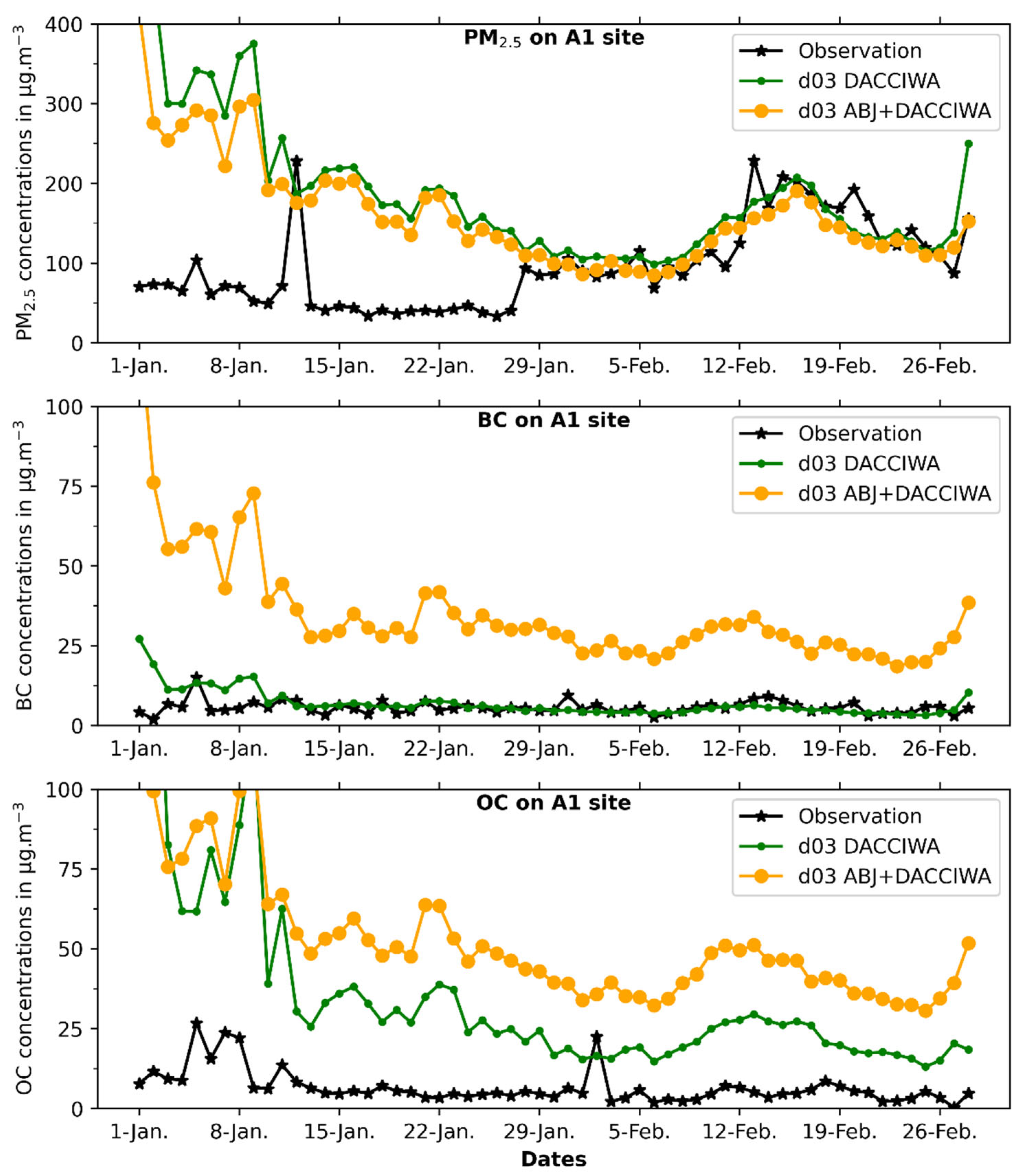
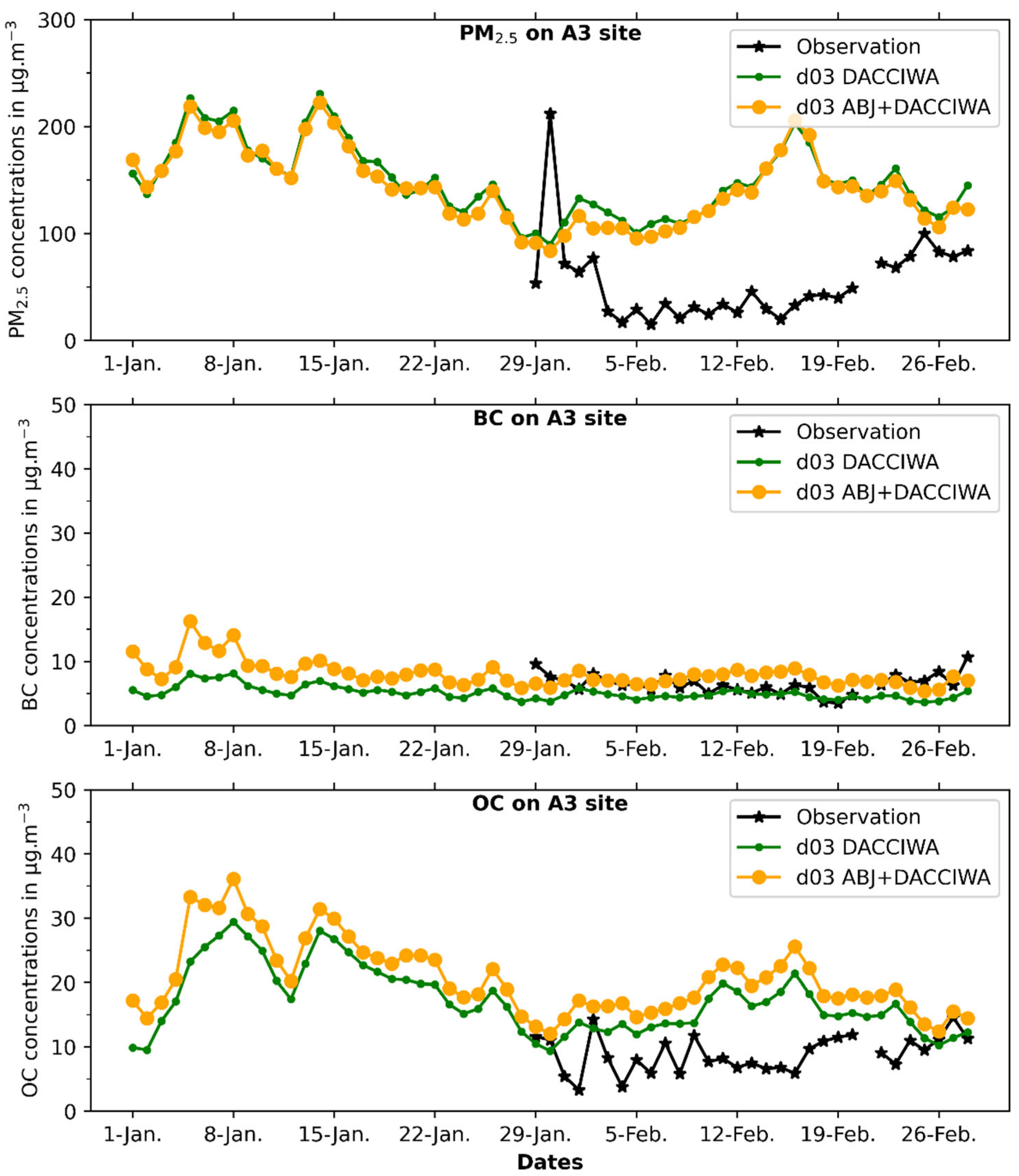
3.2.1. Evaluation of City-Scale Modeling vs. Observations

Figure 4 shows the comparison between the WRF-Chem-simulated concentrations against the corresponding PM₁₀ and PM_2.5 observations from 20 measurement sites sampled by the Abidjan 2019 intensive campaign and published by Gnamien et al. [11]. The observations are represented with black squares; the simulations based on the DACCIWA inventory are in green; and the simulations based on the ABJ+DACCIWA inventory are in orange. Both the simulations for all the domains overestimate, in general, the PM₁₀ and PM_2.5 concentrations at the sites observed by Gnamien et al. [11], except for some sites, A7, A8, A9, A18, and A20, for PM₁₀, and A7, A9, A12, and A20, for PM_2.5, where they are underestimated. These sites, which are either close to high-traffic roads or close to industrial areas, are under the influence of road dust, a source not included in the model.

The results for PM₁₀ show that the simulations performed in the d01 domain (25 km × 25 km) based on the ABJ+DACCIWA inventory as well as in the d03 domain with the ABJ+DACCIWA inventory perform the best as compared with observations. The worst agreement between the modeled and observed concentrations occur at most of the sites for the d02 and d03 simulations using the DACCIWA inventory. On the other hand, for PM_2.5, the simulations of the d03 domain with the ABJ+DACCIWA inventories give values generally higher than the other simulations, whereas concentrations obtained for the d01 domain with the ABJ+DACCIWA inventory are, most of the time, closer to the observations than the other domains, as for PM₁₀. These differences can be due to several factors, like inability of the model to adequately resolve micro-scale processes, uncertainties in different emission sources, lack of nitrate in the GOCART model, SOA parametrization, and numerical approximations.

The root mean squared error (RMSE) and the coefficients of variation of the errors (biases) of the simulated PM₁₀ and PM_2.5 with respect to the observations of all the sites of the Abidjan intensive campaign have been calculated.

Table 5. Root mean squared error (RMSE) between model output and observations from Gnamien et al. 2020 [11].

Simulation Domain	Simulated Inventory	RMSE (µg.m−3)
		PM10	PM2.5
d01	DACCIWA	62.0	48.8
	ABJ+DACCIWA	45.8	31.2
d02	DACCIWA	86.5	69.4
	ABJ+DACCIWA	62.8	48.8
d03	DACCIWA	63.9	78.8
	ABJ+DACCIWA	52.9	68.2

allows us to compare the performance of the WRF-Chem model with both of the inventories, i.e., DACCIWA and ABJ+DACCIWA, but also the impact of increased spatial resolution of the simulations on the errors. The biases of all the simulations are negative, as the model overestimates the observations for most sites.

The RMSE of the simulations based on the DACCIWA inventories are always higher than those of the simulations based on the ABJ+DACCIWA inventories, by 26%, 27%, and 17%, respectively, for simulations at d01, d02, and d03 for PM10, and 18%, 21%, and 11% for PM_2.5. The same is true for the biases, where decreases of 43%, 30%, and 31% are observed for PM₁₀, and 54%, 32%, and 17% for PM_2.5. These estimates confirm that the values from the simulations based on the city scale inventory (ABJ+DACCIWA) are closer to the observations compared to those simulated using the DACCIWA inventory. However, in general, the RMSE values and biases for PM_2.5 increase with increasing model resolution. A similar result was obtained by [48] for PM₁₀ simulations with the WRF-Chem model over West Africa in the Sahelian zone, which supports the hypothesis that the impact of microscale processes on PM₂.₅ are likely not well represented [49]. However, in our study, no particular variation is observed for PM₁₀, unlike [48], in which study sites were impacted more by dust of regional origin [49].

Next, we compared the observed and modeled values of PM_2.5, BC, and OC concentrations obtained in Abidjan in January 2019 from daily filter sampling [10] during the PASMU campaign at two sites: site A1: Cocody: University Felix Houphouet-Boigny, (5.35° N, 3.99° E) and site A3: TREICHVILLE—Nanan Yamousso, (5.31° N, 4.01° E). These two sites are considered urban-type sites.

Figure 5 shows the time series of PM_2.5, BC, and OC concentrations, simulated on the basis of the DACCIWA (green) and ABJ+DACCIWA (orange) inventories, for d03 (1 km × 1 km) at site A1 from 1 January to 28 February 2019.

As shown in Figure 4, differences between observed and simulated PM_2.5 concentrations may be noticed during January 2019. However, during February 2019, the model manages to more accurately simulate PM_2.5 concentrations, with better results for the d03 domain. Moreover, the difference between the d03 simulation results for the two inventories give similar profiles, with a gap that decreases with increasing the spatial resolution of the model.

Concerning the BC, the WRF-Chem model manages to reproduce the order of magnitude of the observations over the whole period (January and February 2019) in both of the simulations and for two domains (d01 and d02). However, the simulation of the d03 domain (Figure 5) largely overestimates the BC concentrations for the ABJ+DACCIWA inventory, while the simulation for the DACCIWA inventory alone well agrees with the observations. As for OC, the simulated data are always higher than the observed data, with the difference increasing with model resolution. The same is true when comparing the differences obtained between the simulations for the two inventories, with worse results for the ABJ+DACCIWA inventory. However, it is interesting to show that the observed and modeled concentration temporal variations agree for all simulations, except for the peak observed on 5 February. As mentioned above, the observed differences for organic carbon may have multiple reasons: treatment of primary and secondary organic carbon in the model; terrain complexity; and local meteorological dynamics [50].

In conclusion, the reliability of the BC simulations for the d01 (25 km × 25 km) and d02 (5 km × 5 km) domains reflects the urban background site characteristics of site A1. The overestimation obtained for the modeling of the d03 (1 km × 1 km) domain with the ABJ+DACCIWA inventory and not with the DACCIWA inventory suggests that fine-scale corrections are needed. Moreover, biases in OC increase with an increase in resolution, while the opposite is observed for PM_2.5, suggesting that the need for further improvements in both the emissions and aerosol chemical composition simulations in the model.

Figure 6 shows the same results as Figure 5, but for site A3. For this site, the observations only cover the period from 29 January to 28 February 2019. We observed that whatever the inventory, the simulations for all the three domains overestimate the PM_2.5 concentrations, with slightly larger values for the simulations based on the DACCIWA inventory for domains d01 and d02. The same observation was made for the OC, but with less important differences, especially with the simulations based on the DACCIWA inventory. On the other hand, it is interesting to note that the simulations of the d02 and d03 domains manage to well reproduce the concentrations observed for the BC with better comparison with the ABJ+DACCIWA inventory at the beginning and end of the studied period. The results with the DACCIWA inventory were better in the middle of the period. This analysis shows once again that sensitivity tests are to be carried out on the aerosol treatment in the model with respect to organic carbon and the PM_2.5 calculation.

3.2.2. Spatial Evaluation of the Model Results

Figure 7 presents maps of the spatialized biases ((observation − model_output)/observations) of the model output biases compared to observations from Gnamien et al. [11]. Biases are presented as percentages from −100% to +100%, with negative values being overestimates. Overall, over the city of Abidjan, the model overestimates PM₁₀ and PM_2.5 concentrations compared to observations over the same period. Overestimates are greater in areas with high population densities, while overestimates are the largest. On the seafront, the biases are between ±20%, which suggest better simulation of marine aerosols. To test this bias, several methods are considered, including spatializing the DACCIWA inventory at a resolution of 1 km × 1 km with the same spatialization keys as the city inventory.

Considering specific local sources, such as road dust resuspension and industrial sources, will improve the spatial variation maps. In addition, sensitivity tests will be conducted to better account for the complexity of the aerosol.

3.3. Spatial Variation Maps

3.3.1. Spatial Variation Maps of PM_2.5 and PM₁₀ Concentrations

Figure 8 shows the spatial distributions of the PM₁₀ and PM_2.5 concentrations simulated by the WRF-Chem model with the ABJ+DACCIWA inventory over the d03 domain, averaged for the period from 20 January to 10 February 2019. It is the combined result of the Abidjan city-scale inventory and the high-resolution simulation of the WRF-Chem model. Only the values extracted from the d03 domain for the city of Abidjan are presented here in order to make a comparison with the spatial maps obtained from the intensive campaign in Abidjan [11]. As shown in Figure 8, the PM₁₀ concentrations are above 100 µg.m⁻³ over the whole study area. For PM_2.5, the obtained values are above 50 µg.m⁻³, and the highest concentrations are observed in the densely populated areas. It is important to note that the minimum values simulated for PM_2.5 and PM₁₀ are well above the WHO air quality guidelines.

Despite the biases observed in the previous paragraph, the city-scale simulation with the WRF-chem model based on the Abidjan city inventory manages to correctly represent the spatial distribution of PM₁₀ and PM_2.5 aerosol concentrations over the city of Abidjan.

The PM₁₀ maps (Figure 8a) from the modeling do not show high concentrations in the south of the study area, but only in the north and in the center, while the observations indicated high concentrations in both the north and in the south [11]. The high concentrations observed in the south (coast) were attributed to marine aerosols and dust from the industrial area. This type of source (industrial dust) was not included in the city inventory due to a lack of information. In addition, in the Abidjan inventory, the emissions from the industrial source located mostly in the south of the area were spatialized using population density, again due to the lack of information on their locations and activity levels. These two reasons may explain the underestimation of PM₁₀ concentrations observed in the south of the area. This problem does not occur for the PM₂.₅ spatial distribution since no PM_2.5 peak is observed along the coast.

It should also be noted that the PM₁₀ and PM_2.5 concentrations north of the area covered by the city inventory are strongly influenced by the DACCIWA inventory. The superposition of the Abidjan inventory (1 km × 1 km) with the DACCIWA inventory (10 km × 10 km) is at the origin of the particularly high emission levels north of Abidjan. Indeed, the spatialization of the DACCIWA inventory, given its 10 times coarser resolution than the Abidjan inventory, artificially attributes high emission values outside the Abidjan study area.

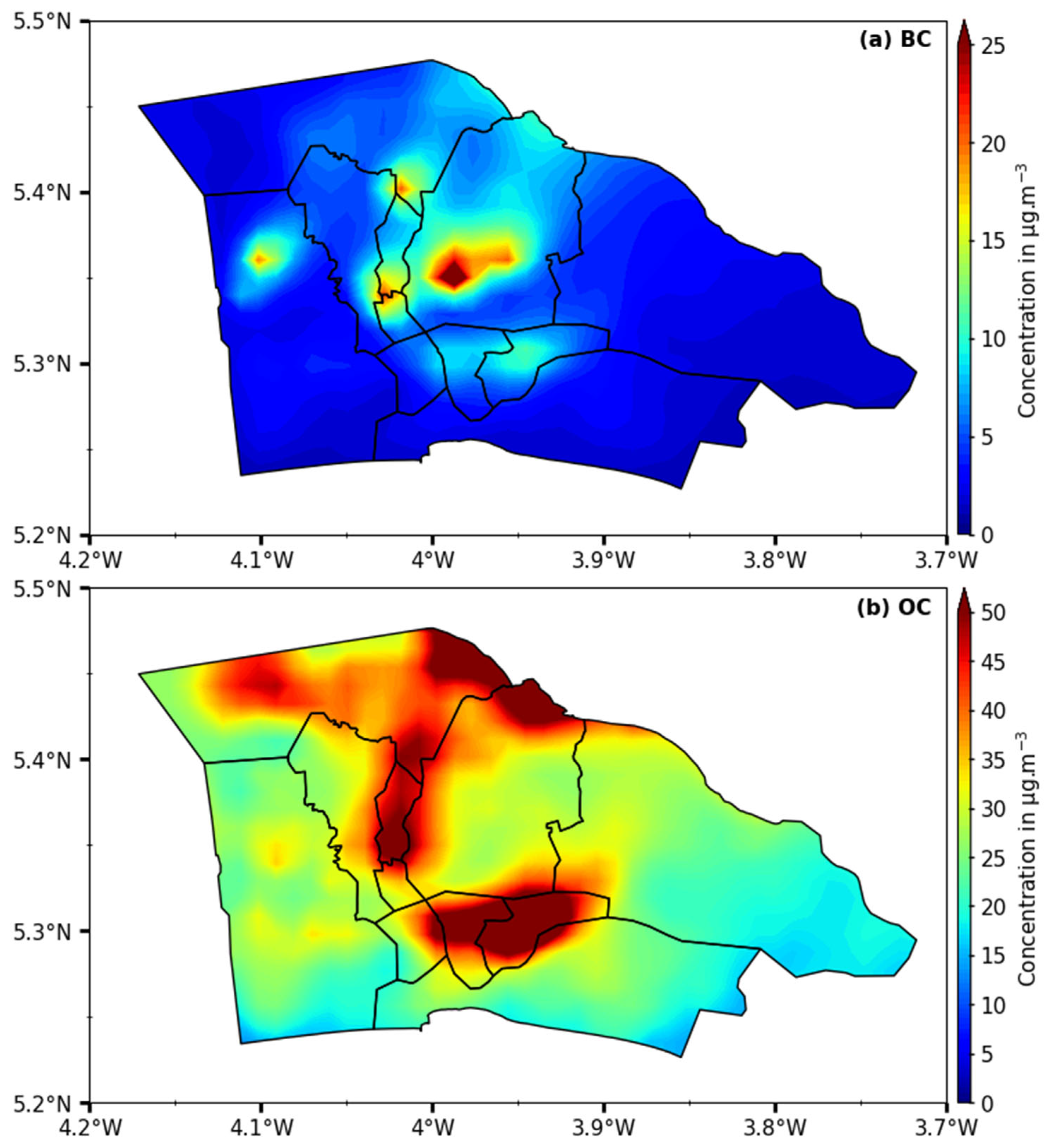
3.3.2. Spatial Variation Maps of BC and OC Concentrations

Carbonaceous aerosol (BC and OC) are important tracers of atmospheric chemistry. Given their importance, numerical atmospheric models consider the atmospheric emissions of these compounds and provide the atmospheric concentrations at the output. Figure 9 shows maps of spatial variations of modeled atmospheric concentrations of carbonaceous aerosol (BC (a) and OC (b)) for the d03 domain with the ABJ+DACCIWA inventory, averaged from 20 January to 10 February 2019. This figure shows that BC concentrations remain lower than OC concentrations (roughly by a factor of two) over the study area. High BC concentrations are observed in the administrative centers of Abidjan due to the high density of road traffic. However, those of OC are more observed in densely populated neighborhoods. This is due to numerous anthropogenic activities, such as domestic fires and waste burning.

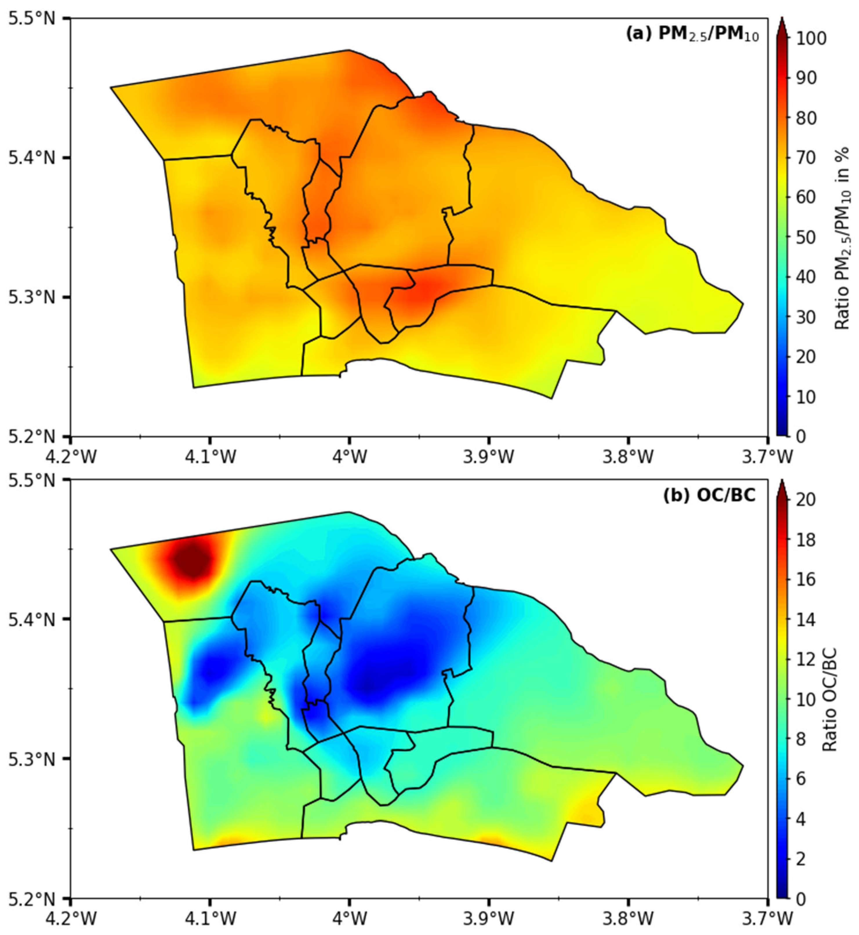
3.3.3. Spatial Variation Maps of the Contribution of PM_2.5 to PM₁₀ Concentrations and of OC/EC Ratios

Figure 10 presents the spatial variation maps of PM_2.5/PM₁₀ ratios in (a) and OC/BC ratios in (b) obtained from modeling at the d03 domain using the ABJ+DACCIWA inventory. The PM_2.5/PM₁₀ ratio represents the relative contribution of PM_2.5 (main anthropogenic aerosols) to PM₁₀ concentrations, which, as a reminder, are all aerosols with diameters (d) less than 10 µm. Therefore, this parameter serves as a tracer for anthropogenic sources. The PM_2.5/PM₁₀ ratios (Figure 10a) are greater than 50% throughout the city of Abidjan, demonstrating the significance of anthropogenic sources in the city. Furthermore, in densely populated areas, the ratio is up to 90% due to multiple sources of pollution (domestic fires, waste fires, traffic, etc.). These values and the spatial distribution of these PM_2.5/PM₁₀ ratios align with the maps created by Gnamien et al. [10] for Abidjan based on observations.

Figure 10b presents the spatial variation map of modeled OC/BC ratios in the city of Abidjan. These ratios range between 1 and 20, with an average of 13.6 ± 1.6, exceeding the value of 1.5 observed by Gnamien et al. (2023) over a longer period in Abidjan, highlighting the significance of OC-emitting sources. In areas of high population density (city center) and intense urbanization, the OC/BC ratio is lower, indicating contributions from both BC-emitting sources (road traffic) and OC sources (domestic and waste fires). The outskirts of Abidjan show lower levels of urbanization and, therefore, less traffic-related sources, resulting in fewer BC emissions and higher OC/EC ratios. This is particularly noticeable in the north-west of Abidjan in the Abobo district. In this popular area, high OC emissions due to intense household combustion activities are also existing. Finally, it is important to note that the overestimation of OC concentrations when comparing model outputs with observations introduces significant uncertainty and may downplay the importance of BC-emitting sources in Abidjan.

4. Summary and Conclusions

This study presents the first fine-scale modeling of particulate pollution in a West African city, Abidjan (Côte d’Ivoire). It provides a methodological framework for fine-scale modeling in West African cities, addressing a major objective of the PASMU project aimed at characterizing urban air pollution and its health impact in Côte d’Ivoire. The modeling is based on a new emission inventory developed specifically for this purpose, incorporating previous works for emission factor selection and utilizing the regional inventory from the DACCIWA program. Special attention was given to the traffic source, considering the unique characteristics of Abidjan’s vehicle fleet. Socio-economic parameters were also employed to update emissions from domestic fires, and the spatialization of emissions was improved with new source-specific keys. This new city-scale inventory for Abidjan (ABJ) was integrated into the DACCIWA inventory for the city area, resulting in the ABJ+DACCIWA inventory.

The total emissions for Abidjan in 2019 amount to 4986.8 Gg of BC, 14,731.4 Gg of OC, and 7751.6 Gg of SO₂, with domestic fires and traffic being the main sources of OC (44%) and BC (52%), respectively. Domestic fires emit 1117.4 Gg of BC and 7719.5 Gg of OC, while traffic emits 2198.8 Gg of BC and 2062.6 Gg of OC. Moreover, 66% of SO₂ emissions are linked to industrial activities.

Simulations were conducted using the WRF-Chem model (simplified GOCART model) based on the ABJ+DACCIWA and DACCIWA inventories. These simulations aimed to study the influence of the ABJ+DACCIWA inventory compared to the regional DACCIWA inventory. Over three domains (from regional to urban), simulations were carried out from January to February 2019, a period with extensive observational databases in Abidjan that have been validated.

Spatialized biases in PM₁₀ and PM_2.5 concentrations compared to observations over Abidjan indicate a general tendency of the WRF-Chem model to overestimate concentrations, especially in densely populated areas, with notable biases along the coastline. The model based on the Abidjan inventory accurately reproduces the spatial distribution of aerosol concentrations determined from observations. Modeled concentration maps of PM₁₀ and PM_2.5 from the ABJ+DACCIWA inventory show high concentrations in densely populated areas, although there is an underestimation of industrial dust effects in the south.

Modeled concentration maps for BC and OC highlight higher BC levels in administrative areas due to road traffic, while OC concentrations are significant in densely populated neighborhoods due to the extensive use of domestic fires and waste burning.

The analysis of PM_2.5/PM₁₀ ratios higher than 50% underscores the dominance of anthropogenic sources in Abidjan, particularly in densely populated areas (up to 90%). The OC/BC ratio (mean value of the order of 14) indicates the predominance of incomplete combustion sources over Abidjan but also shows strong variations across the city, indicating diverse relative contributions of the different combustion-related pollution sources. Given the crucial role of carbonaceous aerosol as atmospheric chemistry tracers, the necessity of sensitivity tests, especially on OC treatment, and consideration of local sources are emphasized to enhance model accuracy in Abidjan. Sensitivity tests are also considered to better understand the impact of different parameterizations on local atmospheric dynamics.

This work proposes a methodology for developing emission inventories and modeling at the scale of African cities, enabling the impact of particulate matter and other air pollutants on air quality and population health to be assessed. Ultimately, this study makes it possible to determine the concentration levels of atmospheric pollutants on the scale of the city using a combination of more precise emission inventories and city-scale modeling, paving the way for air quality forecasting and the implementation of health and climate plans in African cities, which are too often lacking in air quality monitoring systems.

References

1. Guillaume, B.; Liousse, C.; Rosset, R.; Cachier, H.; Van Velthoven, P.; Bessagnet, B.; Poisson, N. ORISAM-TM4: A New Global Sectional Multi-Component Aerosol Model Including SOA Formation—Focus on Carbonaceous BC and OC Aerosols. Tellus B 2007, 59, 283–302. [Google Scholar] [CrossRef]
2. Liousse, C.; Guillaume, B.; Grégoire, J.M.; Mallet, M.; Galy, C.; Pont, V.; Akpo, A.; Bedou, M.; Castéra, P.; Dungall, L.; et al. Updated African Biomass Burning Emission Inventories in the Framework of the AMMA-IDAF Program, with an Evaluation of Combustion Aerosols. Atmos. Chem. Phys. 2010, 10, 9631–9646. [Google Scholar] [CrossRef]
3. Malavelle, F.; Mallet, M.; Pont, V.; Liousse, C.; Solmon, F. Long-Term Simulations (2001–2006) of Biomass Burning and Mineral Dust Optical Properties over West Africa: Comparisons with New Satellite Retrievals. Atmos. Chem. Phys. 2011, 11, 28587–28626. [Google Scholar] [CrossRef]
4. Menut, L.; Bessagnet, B.; Khvorostyanov, D.; Turquety, S.; Monge, J.-L.; Valari, M.; Vautard, R. Modélisation de La Composition Chimique de La Troposphère Avec CHIMERE. Météorologie 2011, 8, 23. [Google Scholar] [CrossRef]
5. Liousse, C.; Assamoi, E.; Criqui, P.; Granier, C.; Rosset, R. Explosive Growth in African Combustion Emissions from 2005 to 2030. Environ. Res. Lett. 2014, 9, 035003. [Google Scholar] [CrossRef]
6. Keita, S.; Liousse, C.; Assamoi, E.-M.; Doumbia, T.; N’Datchoh, E.T.; Gnamien, S.; Elguindi, N.; Granier, C.; Yoboué, V. African Anthropogenic Emissions Inventory for Gases and Particles from 1990 to 2015. Earth Syst. Sci. Data 2021, 13, 3691–3705. [Google Scholar] [CrossRef]
7. WHO. Lignes Directrices OMS Relatives à la Qualité de L’air: Particules, Ozone, Dioxyde D’azote et Dioxyde de Soufre; Organisation Mondiale de la Santé: Genève, Switzerland, 2021. [Google Scholar]
8. Adon, A.J.; Liousse, C.; Doumbia, E.T.; Baeza-Squiban, A.; Cachier, H.; Léon, J.-F.; Yoboue, V.; Akpo, A.B.; Galy-Lacaux, C.; Zoutien, C.; et al. Physico-Chemical Characterization of Urban Aerosols from Specific Combustion Sources in West Africa at Abidjan in Côte d’Ivoire and Cotonou in Benin in the Frame of DACCIWA Program. Atmos. Chem. Phys. 2020, 20, 1–69. [Google Scholar] [CrossRef]
9. Djossou, J.; Léon, J.-F.; Akpo, A.B.; Liousse, C.; Yoboué, V.; Bedou, M.; Bodjrenou, M.; Chiron, C.; Galy-Lacaux, C.; Gardrat, E.; et al. Mass Concentration, Optical Depth and Carbon Composition of Particulate Matter in the Major Southern West African Cities of Cotonou (Benin) and Abidjan (Côte d’Ivoire). Atmos. Chem. Phys. 2018, 18, 6275–6291. [Google Scholar] [CrossRef]
10. Gnamien, S.; Liousse, C.; Keita, S.; Silue, S.; Bahino, J.; Gardrat, E.; Kassamba-Diaby, M.L.; Ochou, A.; Yoboue, V. Chemical Characterization of Urban Aerosols in Abidjan and Korhogo (Cote d’Ivoire) from 2018 to 2020 and Identification of Their Potential Emission Sources. Environ. Sci. Atmos. 2023, 3, 1741–1757. [Google Scholar] [CrossRef]
11. Gnamien, S.; Yoboué, V.; Liousse, C.; Ossohou, M.; Keita, S.; Bahino, J.; Siélé, S.; Diaby, L. Particulate Pollution in Korhogo and Abidjan (Cote d’Ivoire) during the Dry Season. Aerosol Air Qual. Res. 2020, 21, 19. [Google Scholar] [CrossRef]
12. Bahino, J.; Yoboué, V.; Galy-Lacaux, C.; Adon, M.; Akpo, A.; Keita, S.; Liousse, C.; Gardrat, E.; Chiron, C.; Ossohou, M.; et al. A Pilot Study of Gaseous Pollutants’ Measurement (NO2, SO2, NH3, HNO3 and O3) in Abidjan, Côte d’Ivoire: Contribution to an Overview of Gaseous Pollution in African Cities. Atmos. Chem. Phys. 2018, 18, 5173–5198. [Google Scholar] [CrossRef]
13. Keita, S.; Liousse, C.; Yoboué, V.; Dominutti, P.; Guinot, B.; Assamoi, E.-M.; Borbon, A.; Haslett, S.L.; Bouvier, L.; Colomb, A.; et al. Particle and VOC Emission Factor Measurements for Anthropogenic Sources in West Africa. Atmos. Chem. Phys. 2018, 18, 7691–7708. [Google Scholar] [CrossRef]
14. Doumbia, M.; Kouassi, A.A.; Silué, S.; Yoboué, V.; Liousse, C.; Diedhiou, A.; Touré, N.E.; Keita, S.; Assamoi, E.-M.; Bamba, A.; et al. Road Traffic Emission Inventory in an Urban Zone of West Africa: Case of Yopougon City (Abidjan, Côte d’Ivoire). Energies 2021, 14, 1111. [Google Scholar] [CrossRef]
15. Doumbia, M.; Toure, N.; Silue, S.; Yoboue, V.; Diedhiou, A.; Hauhouot, C. Emissions from the Road Traffic of West African Cities: Assessment of Vehicle Fleet and Fuel Consumption. Energies 2018, 11, 2300. [Google Scholar] [CrossRef]
16. Kassamba-Diaby, M.L.; Galy-Lacaux, C.; Yoboué, V.; Hickman, J.E.; Mouchel-Vallon, C.; Jaars, K.; Gnamien, S.; Konan, R.; Gardrat, E.; Silué, S. The Chemical Characteristics of Rainwater and Wet Atmospheric Deposition Fluxes at Two Urban Sites and One Rural Site in Côte d’Ivoire. Atmosphere 2023, 14, 809. [Google Scholar] [CrossRef]
17. Konan, B.R.; Yoboue, V.; Adiaffi, B.; Diaby, M.; Oga, Y.M.S.; Bakayoko, A.; Gnamien, S.; Keita, S.; Bahino, J.; Ossohou, M. Source of Polycyclic Aromatic Hydrocarbons (PAHs) in Rainwater and Effect on the Health of the Population: The Case of the District of Abidjan in the South of Ivory Coast. J. Water Health 2022, 20, 985–1004. [Google Scholar] [CrossRef] [PubMed]
18. Coulibaly, M.; Attoh-Toure, H.; Kouao, A.R.K.; Kouassi, D.P.; Yéo, S.; Yoboue, V.; Tiembré, I. Impairment in Lung Function among Residents in the Vicinity of an Artisanal Smoking Site in Abidjan Côte d’Ivoire. J. Community Med. Public Health Rep. 2021, 2, 1–9. [Google Scholar] [CrossRef]
19. Evilafo, L.; Kéita, S.; Bahino, J.; Koffi, U.; Koffi, E.; Coulibaly, K.; Yoboue, V.; Ossey, Y.; Djaman, J.; Anin Atchibri, L.; et al. Link between the Combustion of Household Waste from Akouédo Landfill, Air Quality and Vitamin A Status among Residents. J. Mater. Environ. Sci. 2019, 10, 1310–1323. [Google Scholar]
20. Kouao, A.R.K.; N’datchoh, E.T.; Yoboue, V.; Silue, S.; Attoh, H.; Coulibaly, M.; Robins, T. Exposure to Indoor and Outdoor Air Pollution among Children under Five Years Old in Urban Area. GJESM 2019, 5, 191–202. [Google Scholar] [CrossRef]
21. Kouao, A.R.K.; Kouadio, K.; Toure, A.H.; Coulibaly, M. Prevalence of Asthma in Children under 5 Years Old Exposed to Air Pollution in Abidjan, (Côte d’Ivoire). Int. J. Recent Sci. Res. 2019, 10, 33353–33358. [Google Scholar]
22. DACCIWA Project. Deliverable D 2.5 Inflammatory Risk Regional Maps of Dynamics-Aerosol-Chemistry-Cloud Interactions in West Africa Project; Karlsruher Institut für Technologie: Karlsruhe, Germany, 2019. [Google Scholar]
23. Deroubaix, A.; Menut, L.; Flamant, C.; Brito, J.; Denjean, C.; Dreiling, V.; Fink, A.; Jambert, C.; Kalthoff, N.; Knippertz, P.; et al. Diurnal Cycle of Coastal Anthropogenic Pollutant Transport over Southern West Africa during the DACCIWA Campaign. Atmos. Chem. Phys. 2019, 19, 473–497. [Google Scholar] [CrossRef]
24. Liousse, C.; Toure, N.; Roblou, L.; Baeza-Squiban, A.; Annesi-Maesano, I. Dynamics-Aerosol-Chemistry-Cloud Interactions in West Africa—Inflammatory Risk Regional Maps; Karlsruher Institut für Technologie: Karlsruhe, Germany, 2019. [Google Scholar]
25. Junker, C.; Liousse, C. A Global Emission Inventory of Carbonaceous Aerosol from Historic Records of Fossil Fuel and Biofuel Consumption for the Period 1860–1997. Atmos. Chem. Phys. 2008, 8, 1195–1207. [Google Scholar] [CrossRef]
26. Konan, Y.G.; Echui, A.D.; Conférence CODATU XVII. Presented at the Mobilité Intelligente, Inclusive et Soutenable Hyderabad. Conférence CODATU XVII, Institute of urban transport, Inde. 2017. Available online: https://www.itf-oecd.org/codatu-xvii-conference (accessed on 22 July 2020).
27. N’guessan, K.N.; N’guessan, Y.; Diango, K.A.; Perilhon, C.; Sako, M.K.; Saraka, K.J. Energy and Environmental Impact of the Abidjanese Way of Life (Côte D’ivoire): A Case Study of Energy Efficiency of Transport Modes. AIP Conf. Proc. 2020, 2307, 020012. [Google Scholar]
28. RGPH. Indicateurs Démographiques; Institut National de la Statistique: Abidjan, Côte d’Ivoire, 2014. [Google Scholar]
29. Columbia University Center for International Earth Science Information Network (CIESIN). 2020. Available online: http://www.ciesin.org (accessed on 23 August 2021).
30. Wiedinmyer, C.; Yokelson, R.J.; Gullett, B.K. Global Emissions of Trace Gases, Particulate Matter, and Hazardous Air Pollutants from Open Burning of Domestic Waste. Environ. Sci. Technol. 2014, 48, 9523–9530. [Google Scholar] [CrossRef]
31. Grell, G.A.; Peckham, S.E.; Schmitz, R.; McKeen, S.A.; Frost, G.; Skamarock, W.C.; Eder, B. Fully Coupled “Online” Chemistry within the WRF Model. Atmos. Environ. 2005, 39, 6957–6975. [Google Scholar] [CrossRef]
32. Fast, J.D.; Gustafson, W.I.; Easter, R.C.; Zaveri, R.A.; Barnard, J.C.; Chapman, E.G.; Grell, G.A.; Peckham, S.E. Evolution of Ozone, Particulates, and Aerosol Direct Radiative Forcing in the Vicinity of Houston Using a Fully Coupled Meteorology-Chemistry-Aerosol Model. J. Geophys. Res. 2006, 111, D21305. [Google Scholar] [CrossRef]
33. Kuik, F.; Lauer, A.; Beukes, J.P.; Van Zyl, P.G.; Josipovic, M.; Vakkari, V.; Laakso, L.; Feig, G.T. The Anthropogenic Contribution to Atmospheric Black Carbon Concentrations in Southern Africa: A WRF-Chem Modeling Study. Atmos. Chem. Phys. 2015, 15, 8809–8830. [Google Scholar] [CrossRef]
34. Kumar, A.; Jiménez, R.; Belalcázar, L.C.; Rojas, N.Y. Application of WRF-Chem Model to Simulate PM10 Concentration over Bogota. Aerosol Air Qual. Res. 2016, 16, 1206–1221. [Google Scholar] [CrossRef]
35. Adefisan, E.A.; Jovita Oghaego, A. Performance Evaluation of WRF-CHEM in Simulating Harmattan Dust over West Africa. J. Climatol. Weather Forecast 2018, 6, 16. [Google Scholar] [CrossRef]
36. Jenkins, G.S.; Gueye, M. WRF 1960–2014 Winter Season Simulations of Particulate Matter in the Sahel: Implications for Air Quality and Respiratory Health. GeoHealth 2018, 2, 248–260. [Google Scholar] [CrossRef]
37. Do, T.N.N.; Ngo, X.T.; Pham, V.H.; Vuong, N.L.; Le, H.A.; Pham, C.T.; Bui, Q.H.; Nguyen, T.N.T. Application of WRF-Chem to Simulate Air Quality over Northern Vietnam. Environ. Sci. Pollut. Res. 2021, 28, 12067–12081. [Google Scholar] [CrossRef] [PubMed]
38. Buchholz, R.R.; Emmons, L.K.; Tilmes, S.; The CESM2 Development Team. CESM2.1/CAM-Chem Instantaneous Output for Boundary Conditions. 2019. Available online: https://wiki.ucar.edu/pages/viewpage.action?pageId=372834733 (accessed on 23 August 2021).
39. Ginoux, P.; Chin, M.; Tegen, I.; Prospero, J.M.; Holben, B.; Dubovik, O.; Lin, S.-J. Sources and Distributions of Dust Aerosols Simulated with the GOCART Model. J. Geophys. Res. Atmos. 2001, 106, 20255–20273. [Google Scholar] [CrossRef]
40. Chin, M.; Ginoux, P.; Kinne, S.; Torres, O.; Holben, B.N.; Duncan, B.N.; Martin, R.V.; Logan, J.A.; Higurashi, A.; Nakajima, T. Tropospheric Aerosol Optical Thickness from the GOCART Model and Comparisons with Satellite and Sun Photometer Measurements. J. Atmos. Sci. 2002, 59, 461–483. [Google Scholar] [CrossRef]
41. Gong, S.L.; Barrie, L.A.; Blanchet, J.-P. Modeling Sea-Salt Aerosols in the Atmosphere: 1. Model Development. J. Geophys. Res. Atmos. 1997, 102, 3805–3818. [Google Scholar] [CrossRef]
42. Freitas, S.R.; Longo, K.M.; Chatfield, R.; Latham, D.; Silva Dias, M.a.F.; Andreae, M.O.; Prins, E.; Santos, J.C.; Gielow, R.; Carvalho, J.A.J. Including the Sub-Grid Scale Plume Rise of Vegetation Fires in Low Resolution Atmospheric Transport Models. Atmos. Chem. Phys. 2007, 7, 3385–3398. [Google Scholar] [CrossRef]
43. Thompson, G.; Field, P.R.; Rasmussen, R.M.; Hall, W.D. Explicit Forecasts of Winter Precipitation Using an Improved Bulk Microphysics Scheme. Part II: Implementation of a New Snow Parameterization. Mon. Weather. Rev. 2008, 136, 5095–5115. [Google Scholar] [CrossRef]
44. Niu, G.-Y.; Yang, Z.-L.; Mitchell, K.E.; Chen, F.; Ek, M.B.; Barlage, M.; Kumar, A.; Manning, K.; Niyogi, D.; Rosero, E.; et al. The Community Noah Land Surface Model with Multiparameterization Options (Noah-MP): 1. Model Description and Evaluation with Local-Scale Measurements. J. Geophys. Res. 2011, 116, D12109. [Google Scholar] [CrossRef]
45. Nakanishi, M.; Niino, H. Development of an Improved Turbulence Closure Model for the Atmospheric Boundary Layer. J. Meteorol. Soc. Jpn. Ser. II 2009, 87, 895–912. [Google Scholar] [CrossRef]
46. Grell, G.A.; Freitas, S.R. A Scale and Aerosol Aware Stochastic Convective Parameterization for Weather and Air Quality Modeling. Atmos. Chem. Phys. 2014, 14, 5233–5250. [Google Scholar] [CrossRef]
47. Iacono, M.J.; Delamere, J.S.; Mlawer, E.J.; Shephard, M.W.; Clough, S.A.; Collins, W.D. Radiative Forcing by Long-Lived Greenhouse Gases: Calculations with the AER Radiative Transfer Models. J. Geophys. Res. 2008, 113, D13103. [Google Scholar] [CrossRef]
48. Gueye, M.; Jenkins, G.S. Investigating the Sensitivity of the WRF-Chem Horizontal Grid Spacing on PM10 Concentration during 2012 over West Africa. Atmos. Environ. 2019, 196, 152–163. [Google Scholar] [CrossRef]
49. Sicard, P.; Crippa, P.; De Marco, A.; Castruccio, S.; Giani, P.; Cuesta, J.; Paoletti, E.; Feng, Z.; Anav, A. High Spatial Resolution WRF-Chem Model over Asia: Physics and Chemistry Evaluation. Atmos. Environ. 2021, 244, 118004. [Google Scholar] [CrossRef]
50. Žabkar, R.; Honzak, L.; Skok, G.; Forkel, R.; Rakovec, J.; Ceglar, A.; Žagar, N. Evaluation of the High Resolution WRF-Chem (v3.4.1) Air Quality Forecast and Its Comparison with Statistical Ozone Predictions. Geosci. Model Dev. 2015, 8, 2119–2137. [Google Scholar] [CrossRef]
Figure 1. Domains simulated with WRF-Chem in this study. The solid white dot shows the center of the domains located in Abidjan.
Atmosphere 15 00758 g001
Figure 2. Summary of the simulations carried out in this study on the basis of the 2 inventories. In red, the inputs and outputs of the model, relating to simulations from ABJ+DACCIWA and in orange, the inputs and outputs of the model, relating to simulations from the DACCIWA inventory.
Atmosphere 15 00758 g002
Figure 3. Spatialized BC, OC, and SO2 emissions in 2019 in Abidjan due to the traffic source.
Atmosphere 15 00758 g003
Figure 4. Comparison of the average PM2.5 and PM10 concentrations simulated by WRF-Chem for all the domains (d01, d02, and d03) and for each of the simulations (DACCIWA and ABJ+DACCIWA), with the observations values obtained during the intensive campaign in Abidjan [11].
Atmosphere 15 00758 g004
Figure 5. Time series of simulated and observed PM2.5, BC, and OC concentrations at site A1 during January and February 2019. The observation were provided by Gnamien et al.2020 [10].
Atmosphere 15 00758 g005
Figure 6. Time series of simulated and observed PM2.5, BC, and OC concentrations at site A3 during January and February of 2019.
Atmosphere 15 00758 g006
Figure 7. Bias maps of modeled (a) PM10 and (b) PM2.5 concentrations compared with observations from Gnamien et al. (2020) [11].
Atmosphere 15 00758 g007
Figure 8. Spatial variation maps of (a) PM10 and (b) PM2.5 surface aerosol concentrations simulated from the ABJ+DACCIWA inventory by the WRF-Chem model and averaged from 20 January to 10 February 2019.
Atmosphere 15 00758 g008
Figure 9. Spatial variation maps of (a) BC and (b) OC surface concentrations simulated with the ABJ+DACCIWA inventory by the WRF-Chem model, averaged from 20 Januar to 10 February 2019.
Atmosphere 15 00758 g009
Figure 10. Spatial variation maps of relative contributions of PM2.5 aerosols to PM10 aerosols (a) and of OC to BC (b) over the d03 domain from 20 January to 10 February 2019.
Atmosphere 15 00758 g010